
Detecting Reinforced Concrete Rebars Using Ground Penetrating Radars
Abstract
:1. Introduction
2. GPR System and Data Processing
3. Experimental program
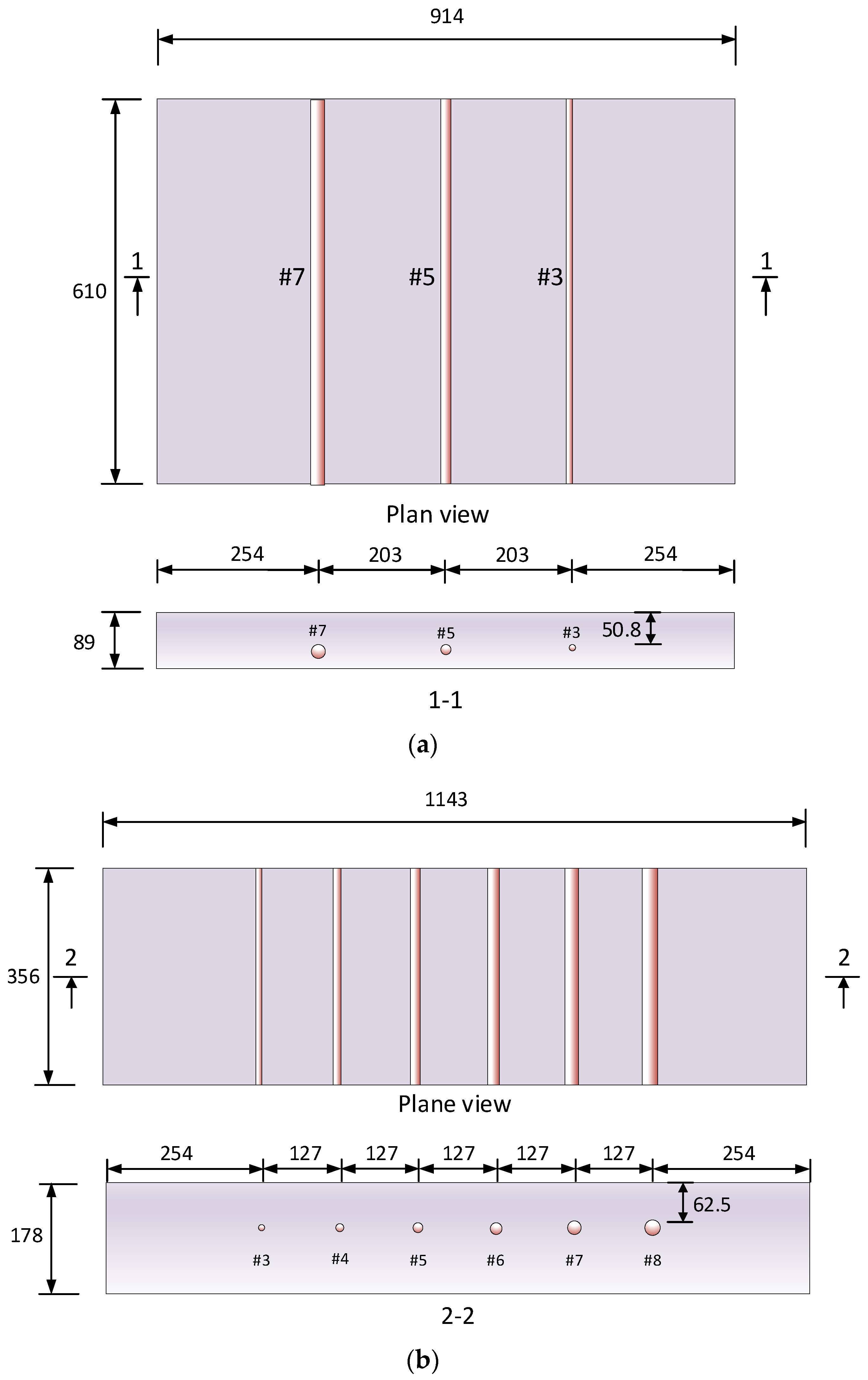
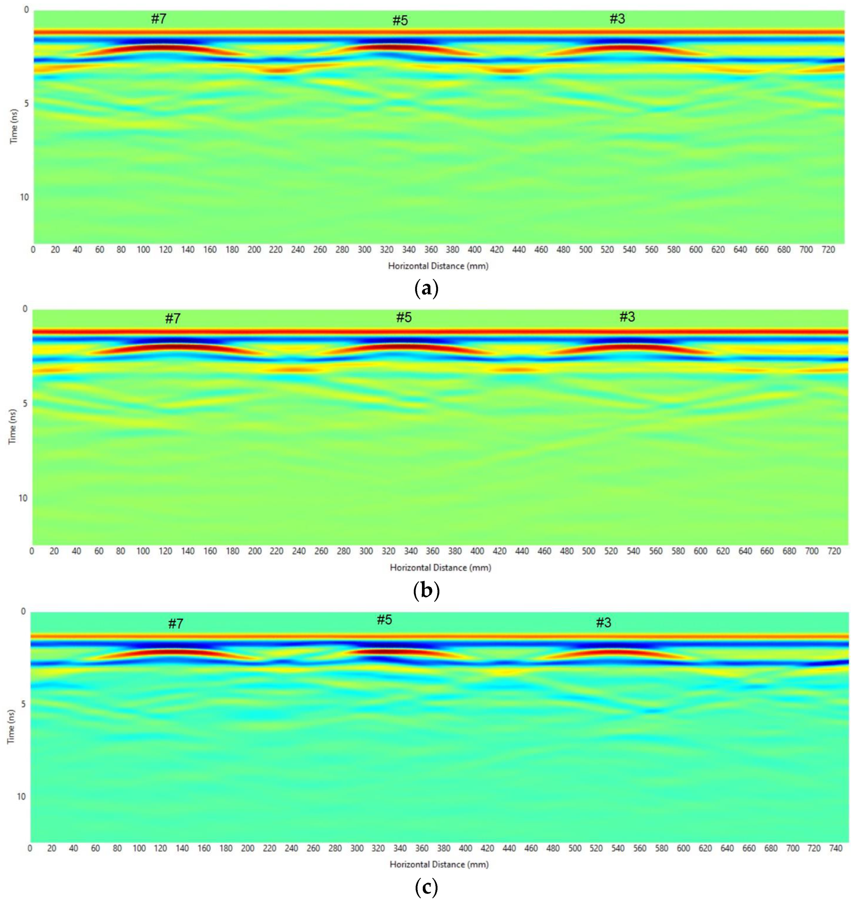
3.1. Specimen Design and Fabrication
3.2. Data Collection and Acquisition
4. Signal Processing
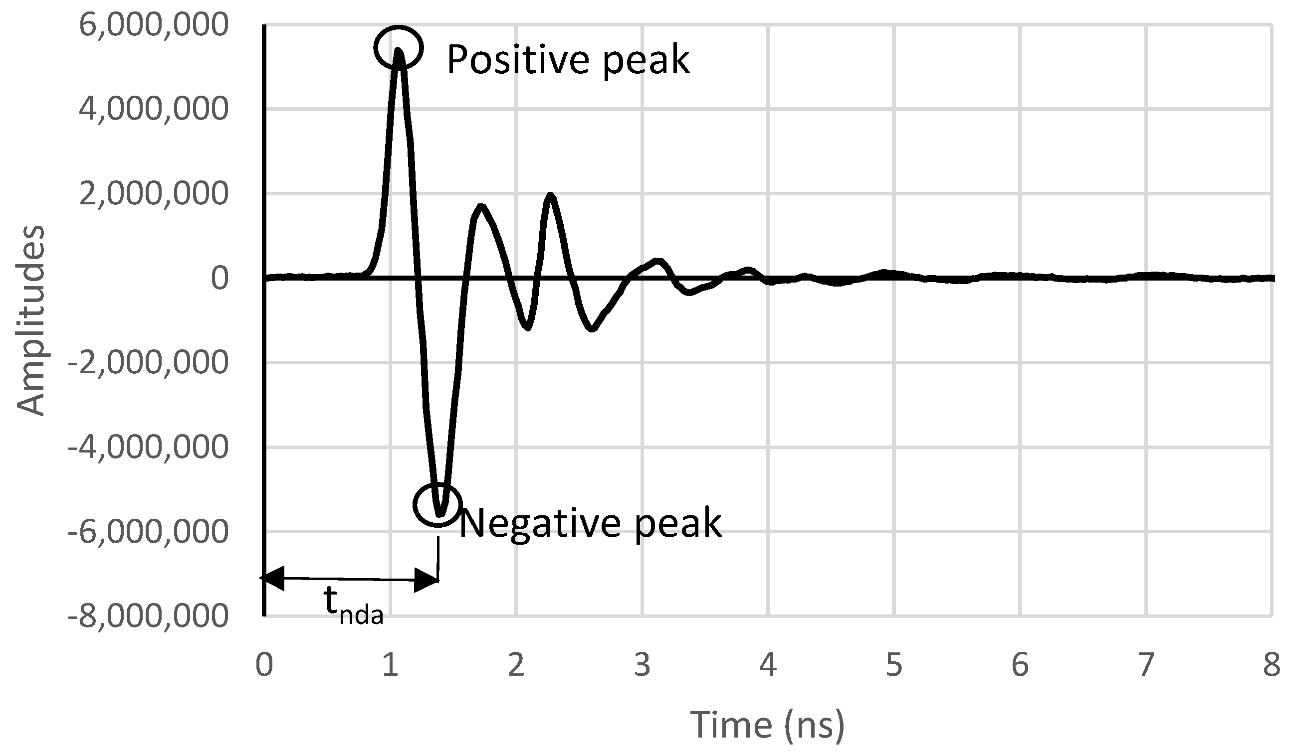
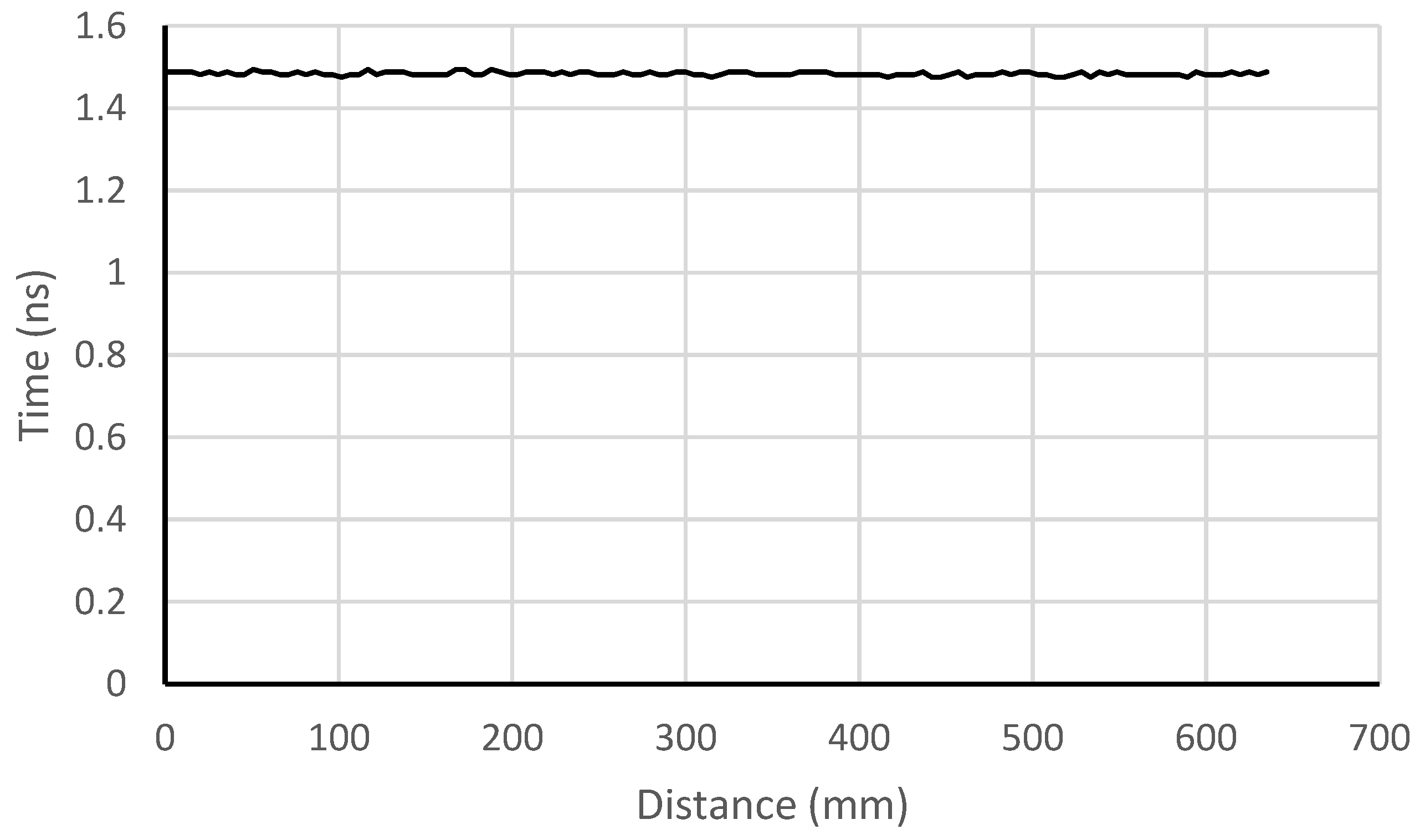
4.1. Time Zero
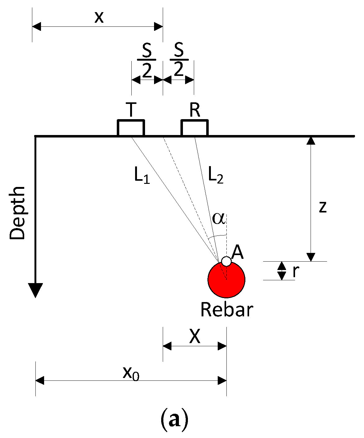
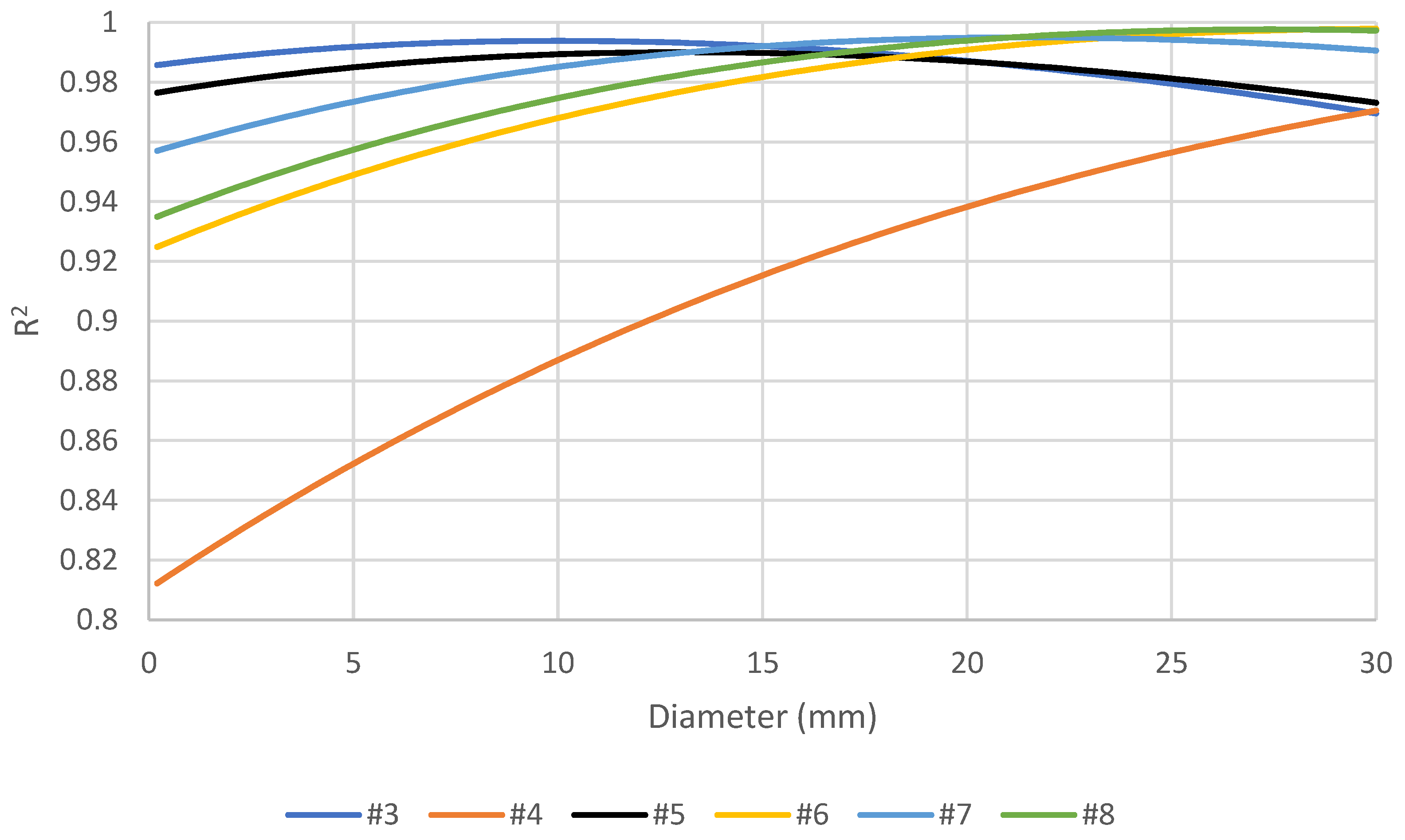
4.2. Rebar Depth and Diameter
- Positive peaks of the reflected waves from rebar correspond to the negative peaks of the transmitting wave (phase reverse).
- The transmitting wave reflects at the surface of the rebar in the shortest two-wave travel path.
- -
- Estimate the electromagnetic wave velocity.
- -
- Calculate the rebar depth using Equation (5).
- -
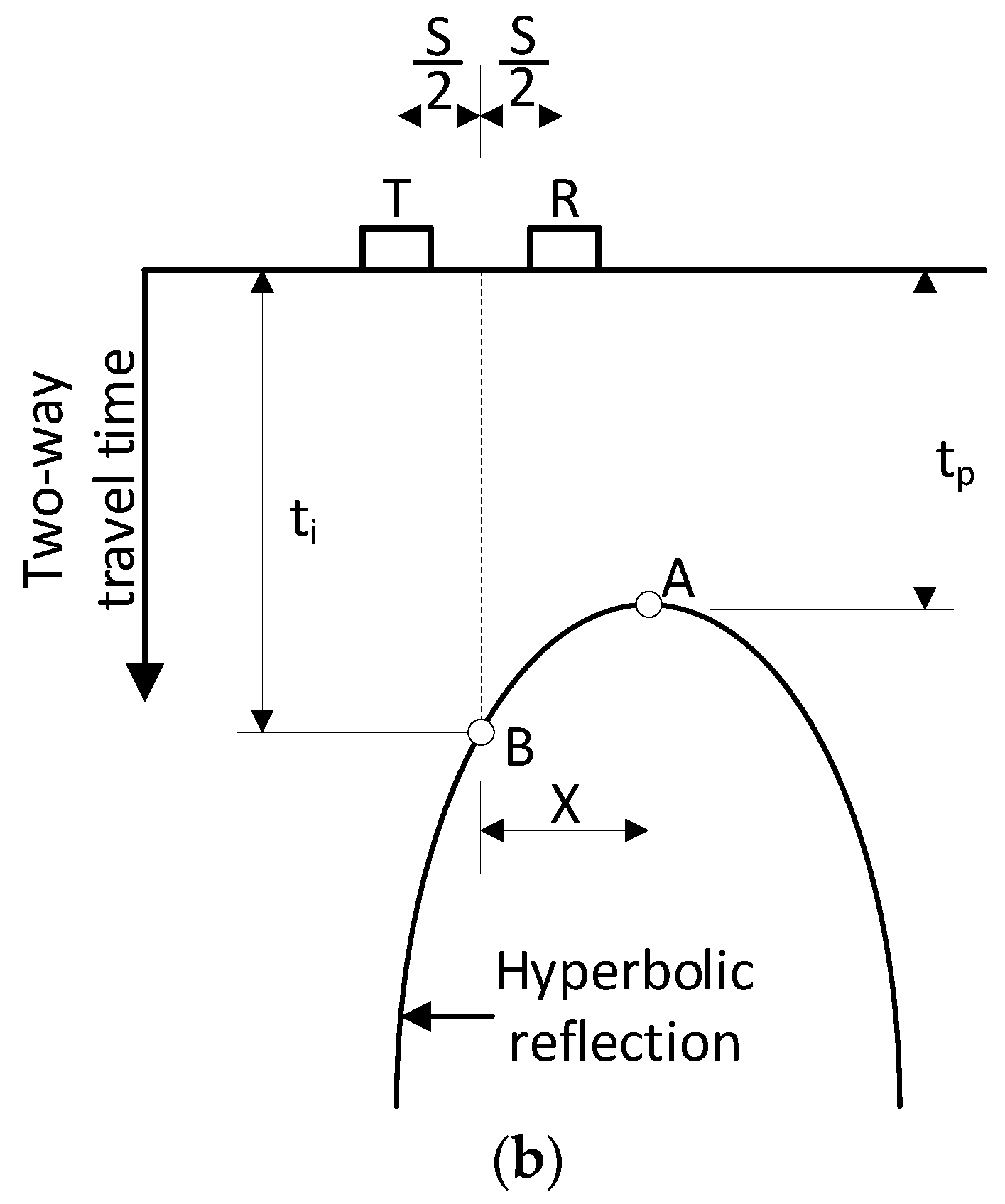
- Identify the coordinates at the peak of the hyperbola.
- -
- Calculate the rebar radius using Equation (7).
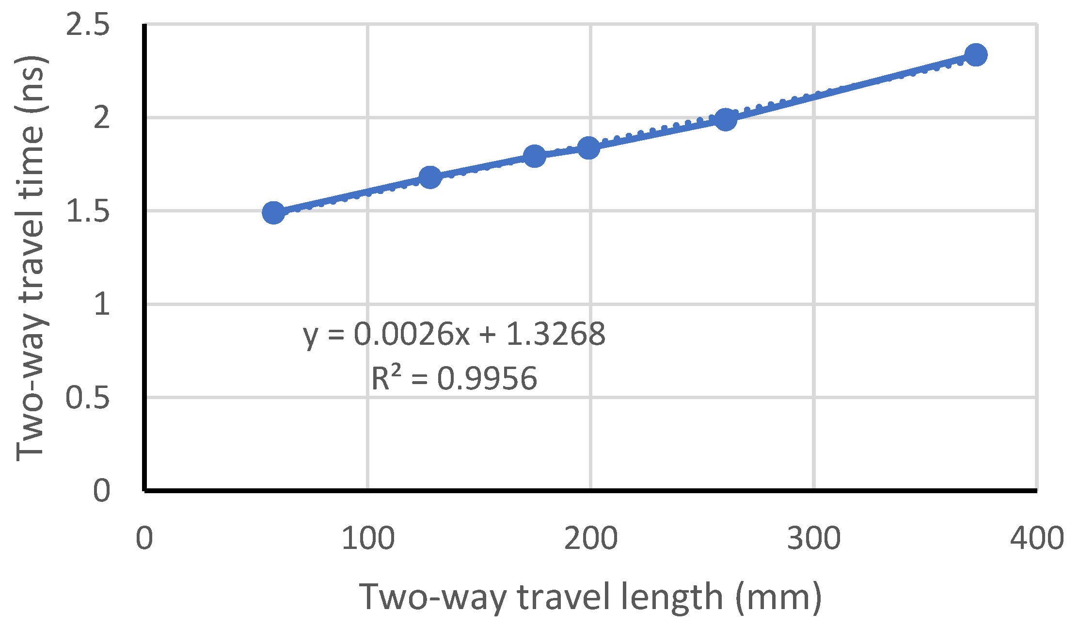
4.3. Wave Velocity
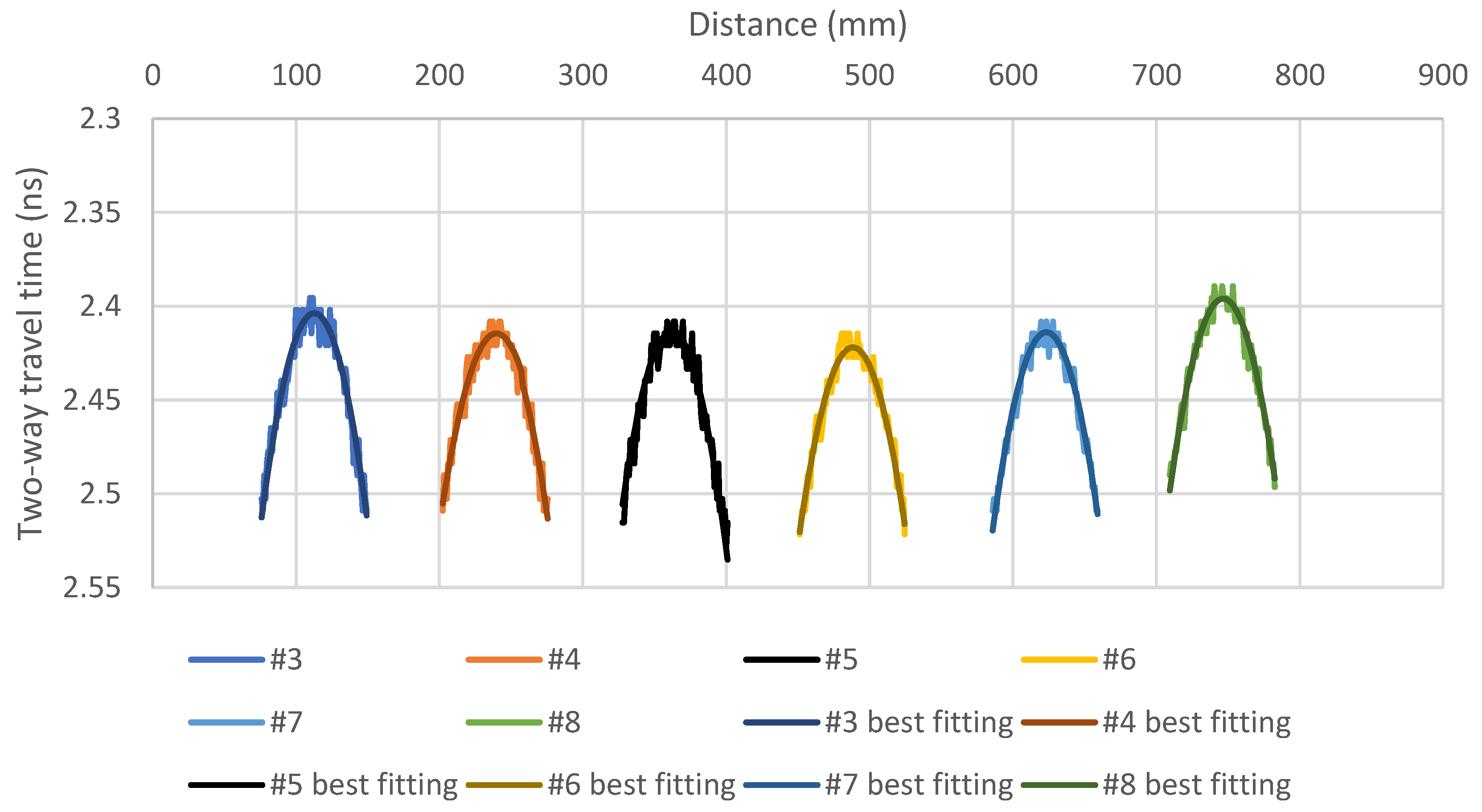
4.4. Determination of the Coordinates at the Peak of the Hyperbola
5. Results and Discussion
6. Conclusions
- Time zero can be accurately determined based on the negative peak of the transmitted signal in the air.
- The thickness of the concrete slab was a reliable indicator for determining the electromagnetic wave.
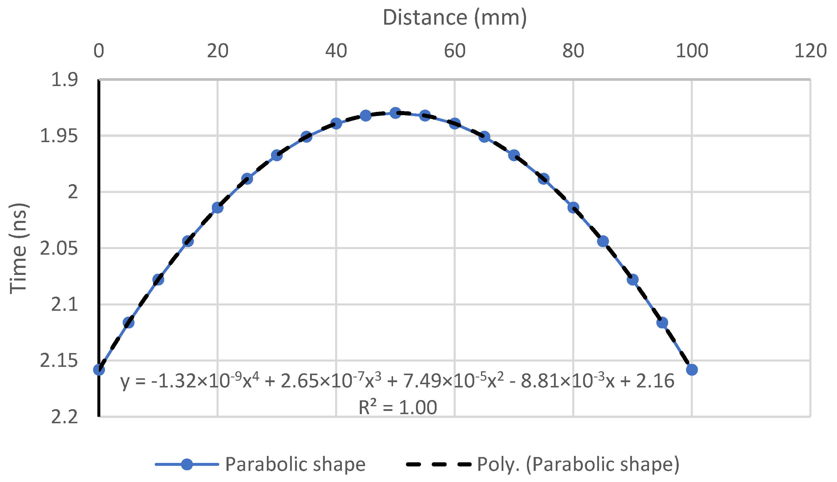
- The biquadratic equation proved to be an efficient method for fitting hyperbolas and estimating both the horizontal location and depth of the rebar.
- The rebar size was successfully estimated with high accuracy using the proposed theoretical equation, provided the reflected hyperbola remained unaffected by adjacent embedded objects.
- The overlapping zone of the rebar reflections may not occur if the minimum spacing of the rebar is approximately 150 mm for rebars #3 to #8.
Author Contributions
Funding
Institutional Review Board Statement
Informed Consent Statement
Data Availability Statement
Acknowledgments
Conflicts of Interest
References
- Zatar, W.A. Assessing the Service Life of Corrosion-Deteriorated Reinforced Concrete Member Highway Bridges in West Virginia; West Virginia Department of Transportation, Division of Highways: Charleston, WV, USA, 2014. [Google Scholar]
- Zatar, W.A.; Harik, I.E.; Sutterer, K.G.; Dodds, A. Bridge Embankments: Part I–Seismic Risk Assessment and Ranking. J. Constr. Facil. 2008, 22, 171–180. [Google Scholar] [CrossRef]
- Zatar, W.A.; Harik, I.E. Bridge Embankments: Part II–Seismic risk for I–24 in Kentucky. J. Constr. Facil. 2008, 22, 181–190. [Google Scholar] [CrossRef]
- Malik, H.; Zatar, W.A. Software agents to support structural health monitoring (SHM)-informed intelligent transportation system (ITS) for bridge condition assessment. Procedia Comput. Sci. 2018, 130, 675–682. [Google Scholar] [CrossRef]
- Malik, H.; Zatar, W.A. Agent–based routing approach to support structural health monitoring–informed, intelligent transportation system. J. Ambient Intell. Humaniz. Comput. 2020, 11, 1031–1043. [Google Scholar] [CrossRef]
- Ren, W.; Zatar, W.A.; Harik, I.E. Ambient vibration-based seismic evaluation of a continuous girder bridge. J. Eng. Struct. 2004, 26, 631–640. [Google Scholar] [CrossRef]
- Xiao, F.; Chen, G.; Zatar, W.A.; Hulsey, L. Signature extraction from the dynamic responses of a bridge subjected to a moving vehicle using complete ensemble empirical mode decomposition. J. Low Freq. Noise Vib. Act. Control 2021, 40, 278–294. [Google Scholar] [CrossRef]
- Xiao, F.; Chen, G.; Husley, L.; Zatar, W.A. Characterization of non-stationary properties of vehicle-bridge response for structural health monitoring. Adv. Mech. Eng. 2017, 9, 1–6. [Google Scholar] [CrossRef]
- Xiao, F.; Chen, G.; Husley, L.; Zatar, W.A. Characterization of nonlinear dynamics for a highway bridge in Alaska. J. Vib. Eng. Technol. 2018, 6, 379–386. [Google Scholar] [CrossRef]
- Kaiser, H.; Karbhari, V.M.; Sikorsky, C. Non-destructive testing techniques for FRP rehabilitated concrete. II: An assessment. Int. J. Mater. Prod. Technol. 2004, 21, 385–401. [Google Scholar] [CrossRef]
- Zatar, W.; Nguyen, H. Condition assessment of ground-mount cantilever weathering-steel overhead sign structures. J. Infrastruct. Syst. 2017, 23, 05017005. [Google Scholar] [CrossRef]
- Büyüköztürk, O. Imaging of concrete structures. NDT E Int. 1998, 31, 233–243. [Google Scholar] [CrossRef]
- Popovics, J.S.; Roesler, J.R.; Bittner, J.; Amirkhanian, A.N.; Brand, A.S.; Gupta, P.; Flowers, K. Ultrasonic Imaging for Concrete Infrastructure Condition Assessment and Quality Assurance; Illinois Center for Transportation/Illinois Department of Transportation: Rantoul, IL, USA, 2017. [Google Scholar]
- Zhu, J.; Wang, Y.; Qing, X. A real-time electromechanical impedance-based active monitoring for composite patch bonded repair structure. Compos. Struct. 2019, 212, 513–523. [Google Scholar] [CrossRef]
- Naoum, M.C.; Sapidis, G.M.; Papadopoulos, N.A.; Voutetaki, M.E. An Electromechanical Impedance-Based Application of Realtime Monitoring for the Load-Induced Flexural Stress and Damage in Fiber-Reinforced Concrete. Fibers 2023, 11, 34. [Google Scholar] [CrossRef]
- Rao, R.K.; Sasmal, S. Electromechanical impedance-based embeddable smart composite for condition-state monitoring. Sens. Actuators A Phys. 2022, 346, 113856. [Google Scholar] [CrossRef]
- Fan, L.; Bao, Y. Review of fiber optic sensors for corrosion monitoring in reinforced concrete. Cem. Concr. Compos. 2021, 120, 104029. [Google Scholar] [CrossRef]
- Berrocal, C.G.; Fernandez, I.; Rempling, R. Crack monitoring in reinforced concrete beams by distributed optical fiber sensors. Struct. Infrastruct. Eng. 2021, 17, 124–139. [Google Scholar] [CrossRef]
- Stanbridge, A.B.; Ewins, D.J. Modal testing using a scanning laser Doppler vibrometer. Mech. Syst. Signal Process. 1999, 13, 255–270. [Google Scholar] [CrossRef]
- ACI Committee 228. Report on Nondestructive Test Methods for Evaluation of Concrete in Structures; Report ACI 228.2R-13; American Concrete Institute: Indianapolis, IN, USA, 2013. [Google Scholar]
- Alani, A.M.; Aboutalebi, M.; Kilic, G. Applications of ground penetrating radar (GPR) in bridge deck monitoring and assessment. J. Appl. Geophys. 2013, 97, 45–54. [Google Scholar] [CrossRef]
- He, X.Q.; Zhu, Z.Q.; Liu, Q.Y.; Lu, G.Y. Review of GPR rebar detection. In Proceedings of the PIERS, Moscow, Russia, 18–21 August 2009; pp. 804–813. [Google Scholar]
- Bala, D.C.; Garg, R.D.; Jain, S.S. Rebar detection using GPR: An emerging non-destructive QC approach. Int. J. Eng. Res. Appl. 2011, 1, 2111–2117. [Google Scholar]
- Hasan, M.I.; Yazdani, N. An experimental study for quantitative estimation of rebar corrosion in concrete using ground penetrating radar. J. Eng. 2016, 2016, 8536850. [Google Scholar] [CrossRef]
- Hugenschmidt, J. Concrete bridge inspection with a mobile GPR system. Constr. Build. Mater. 2002, 16, 147–154. [Google Scholar] [CrossRef]
- Hasan, M.I.; Yazdani, N. Ground penetrating radar utilization in exploring inadequate concrete covers in a new bridge deck. Case Stud. Constr. Mater. 2014, 1, 104–114. [Google Scholar] [CrossRef]
- Zhou, F.; Chen, Z.; Liu, H.; Cui, J.; Spencer, B.F.; Fang, G. Simultaneous estimation of rebar diameter and cover thickness by a GPR-EMI dual sensor. Sensors 2018, 18, 2969. [Google Scholar] [CrossRef] [PubMed]
- Laurens, S.; Balayssac, J.P.; Rhazi, J.; Klysz, G.; Arliguie, G. Non-destructive evaluation of concrete moisture by GPR: Experimental study and direct modeling. Mater. Struct. 2005, 38, 827–832. [Google Scholar] [CrossRef]
- Gucunski, N.; Rascoe, C.; Parrillo, R.; Roberts, R.L. Complementary Condition Assessment of Bridge Decks by High-Frequency Ground-Penetrating Radar and Impact Echo. No. 09-1282. 2009. Available online: https://trid.trb.org/View/881090 (accessed on 19 May 2009).
- Benedetto, A.; Manacorda, G.; Simi, A.; Tosti, F. Novel perspectives in bridges inspection using GPR. Nondestruct. Test. Eval. 2012, 27, 239–251. [Google Scholar] [CrossRef]
- Eisenmann, D.; Margetan, F.; Chiou, C.P.T.; Roberts, R.; Wendt, S. Ground penetrating radar applied to rebar corrosion inspection. In AIP Conference Proceedings; American Institute of Physics: College Park, MD, USA, 2013; Volume 1511, No. 1; pp. 1341–1348. [Google Scholar]
- Zaki, A.; Johari, M.; Azmi, M.; Hussin, W.; Aminuddin, W.M.; Jusman, Y. Experimental Assessment of Rebar Corrosion in Concrete Slab Using Ground Penetrating Radar (GPR). Int. J. Corros. 2018, 2018, 5389829. [Google Scholar] [CrossRef]
- Eisenmann, D.; Margetan, F.J.; Koester, L.; Clayton, D. Inspection of a large concrete block containing embedded defects using ground penetrating radar. In AIP Conference Proceedings; AIP Publishing LLC: Long Island, NY, USA, 2016; Volume 1706, p. 020014. [Google Scholar]
- Garg, S.; Misra, S. Efficiency of NDT techniques to detect voids in grouted post-tensioned concrete ducts. Nondestruct. Test. Eval. 2020, 36, 366–387. [Google Scholar] [CrossRef]
- Yehia, S.; Qaddoumi, N.; Farrag, S.; Hamzeh, L. Investigation of concrete mix variations and environmental conditions on defect detection ability using GPR. NDT E Int. 2014, 65, 35–46. [Google Scholar] [CrossRef]
- Tarussov, A.; Vandry, M.; De La Haza, A. Condition assessment of concrete structures using a new analysis method: Ground-penetrating radar computer-assisted visual interpretation. Constr. Build. Mater. 2013, 38, 1246–1254. [Google Scholar] [CrossRef]
- Zatar, W.A.; Nghiem, H.M.; Nguyen, H.D. Effects of antenna frequencies on detectability and reconstructed image of embedded objects in concrete structures using ground-penetrating radar. In Proceedings of the 9th Forensic Engineering Congress, Denver, CO, USA, 4–7 November 2022. [Google Scholar]
- Zatar, W.A.; Nguyen, H.D.; Nghiem, H.M. FRP Retrofitting and Non-Destructive Evaluation for Corrosion-Deteriorated Bridges in West Virginia. Spec. Publ. 2021, 346, 11–30. [Google Scholar]
- Zatar, W.A.; Nguyen, H.D.; Nghiem, H.M.; Cosgun, C. Non-Destructive Testing of GFRP-Wrapped Reinforced-Concrete Slabs. In Proceedings of the Transportation Research Board 100th Annual Meeting, Washington, DC, USA, 5–29 January 2021. No. TRBAM-21-03354. [Google Scholar]
- Zatar, W.; Nghiem, H. Detectability of embedded defects in FRP strengthened concrete deck slabs. In Risk-Based Strategies for Bridge Maintenance; CRC Press: Boca Raton, FL, USA, 2023; pp. 221–234. [Google Scholar]
- Hugenschmidt, J.; Kalogeropoulos, A.; Soldovieri, F.; Prisco, G. Processing strategies for high-resolution GPR concrete inspections. NDT E Int. 2010, 43, 334–342. [Google Scholar] [CrossRef]
- Zatar, W.; Nguyen, T.; Nguyen, H. Environmental effects on condition assessments of concrete structures with ground penetrating radar. J. Appl. Geophys. 2022, 203, 104713. [Google Scholar] [CrossRef]
- Zatar, W.A.; Nguyen, T.; Nguyen, H.D. Predicting GPR signals from concrete structures using artificial intelligence-based method. Adv. Civ. Eng. 2021, 2021, 6610805. [Google Scholar] [CrossRef]
- Zatar, W.A.; Nguyen, H.D.; Nghiem, H.M. Ultrasonic pitch and catch technique for non-destructive testing of reinforced concrete slabs. J. Infrastruct. Preserv. Resil. 2020, 1, 12. [Google Scholar] [CrossRef]
- Chang, C.W.; Lin, C.H.; Lien, H.S. Measurement radius of reinforcing steel bar in concrete using digital image GPR. Constr. Build. Mater. 2009, 23, 1057–1063. [Google Scholar] [CrossRef]
- Utsi, V.; Utsi, E. Measurement of reinforcement bar depths and diameters in concrete. In Proceedings of the Tenth International Conference on Grounds Penetrating Radar, Delft, The Netherlands, 21–24 June 2004; pp. 659–662. [Google Scholar]
- Zhan, R.; Xie, H. GPR measurement of the diameter of steel bars in concrete specimens based on the stationary wavelet transform. Insight-Non-Destr. Test. Cond. Monit. 2009, 51, 151–155. [Google Scholar] [CrossRef]
- Wiwatrojanagul, P.; Sahamitmongkol, R.; Tangtermsirikul, S.; Khamsemanan, N. A new method to determine locations of rebars and estimate cover thickness of RC structures using GPR data. Constr. Build. Mater. 2017, 140, 257–273. [Google Scholar] [CrossRef]
- Xiang, Z.; Ou, G.; Rashidi, A. Integrated approach to simultaneously determine 3D location and size of rebar in GPR data. J. Perform. Constr. Facil. 2020, 34, 04020097. [Google Scholar] [CrossRef]
- Xiang, Z.; Ou, G.; Rashidi, A. An Innovative Approach to Determine Rebar Depth and Size by Comparing GPR Data with a Theoretical Database. In Construction Research Congress; American Society of Civil Engineers: Reston, VA, USA, 2020; pp. 86–95. [Google Scholar]
- GSSI. Concrete Handbook, GPR Inspection of Concrete. Available online: https://www.geophysical.com/wp-content/uploads/2017/10/GSSI-Concrete-Handbook.pdf (accessed on 1 October 2017).


| Parameters | Unit | Value | Description |
|---|---|---|---|
| SPN | - | 512–16,384 | Samples per scan |
| SPD | - | Varies | Scan per second |
| SPM (Ns) | - | 196.85–1000 | Scan per meter |
| Top position | m | 0.08 | Level of the antenna |
| Range | m | 0.8 | Scan depth |
| Scan spacing | mm | Varies | Scan spacing in a scan line |
| Antenna frequency | GHz | 1.6 | |
| T-R offset | mm | 58 | Distance between transmitter and receiver |
| Slab | Rebar No./Diameter (mm) | Designed Depth (mm) | Calculated Diameter/Depth (mm) | Diameter/Depth Differences (%) |
|---|---|---|---|---|
| S1-1 | #3/9.525 | 50.8 | 10/48 | 5.0/5.5 |
| #5/15.875 | 50.8 | (-)/47 | (-)/7.5 | |
| #7/22.225 | 50.8 | 22.2/48 | 0.1/5.5 | |
| S1-2 | #3/9.525 | 50.8 | 10.4/49 | 9.2/3.5 |
| #5/15.875 | 50.8 | 16/48 | 0.8/5.5 | |
| #7/22.225 | 50.8 | 22.2/49 | 0.1/3.5 | |
| S1-3 | #3/9.525 | 50.8 | 8.6/47 | 9.7/7.5 |
| #5/15.875 | 50.8 | (-)/48 | (-)/5.5 | |
| #7/22.225 | 50.8 | 23.8/47 | 7.1/7.5 |
| Slab | Adjacent Rebar | Calculated Spacing (mm) | Difference (%) |
|---|---|---|---|
| S1-1 | #3–#5 | 214 | 5.4 |
| #5–#7 | 202 | 0.5 | |
| S1-2 | #3–#5 | 205 | 1.0 |
| #5–#7 | 202 | 0.5 | |
| S1-3 | #3–#5 | 206 | 1.5 |
| #5–#7 | 198 | 2.5 |
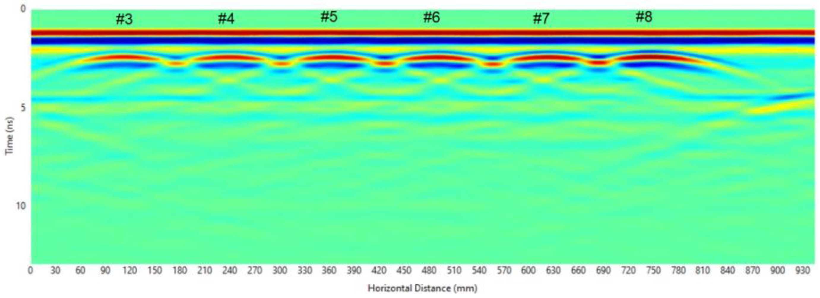
| Rebar No./Diameter (mm) | Designed Depth (mm) | Calculated Diameter/Depth (mm) | Diameter/Depth Differences (%) |
|---|---|---|---|
| #3/9.525 | 62.5 | 10/68 | 5.0/8.8 |
| #4/12.700 | 62.5 | (-)/68 | (-)/8.8 |
| #5/15.875 | 62.5 | 13.2/68 | 16.6/8.8 |
| #6/19.050 | 62.5 | (-)/68 | (-)/8.8 |
| #7/22.225 | 62.5 | 21/68 | 5.5/8.8 |
| #8/25.400 | 62.5 | 27/67 | 6.0/7.2 |
| Adjacent Rebar | Calculated Spacing (mm) | Difference (%) |
|---|---|---|
| #3–#4 | 127 | 0.0 |
| #4–#5 | 122 | 3.9 |
| #5–#6 | 127 | 0.0 |
| #6–#7 | 135 | 6.3 |
| #7–#8 | 123 | 3.1 |
Disclaimer/Publisher’s Note: The statements, opinions and data contained in all publications are solely those of the individual author(s) and contributor(s) and not of MDPI and/or the editor(s). MDPI and/or the editor(s) disclaim responsibility for any injury to people or property resulting from any ideas, methods, instructions or products referred to in the content. |
© 2024 by the authors. Licensee MDPI, Basel, Switzerland. This article is an open access article distributed under the terms and conditions of the Creative Commons Attribution (CC BY) license (https://creativecommons.org/licenses/by/4.0/).
Share and Cite
Zatar, W.; Nghiem, H.; Nguyen, H. Detecting Reinforced Concrete Rebars Using Ground Penetrating Radars. Appl. Sci. 2024, 14, 5808. https://doi.org/10.3390/app14135808
Zatar W, Nghiem H, Nguyen H. Detecting Reinforced Concrete Rebars Using Ground Penetrating Radars. Applied Sciences. 2024; 14(13):5808. https://doi.org/10.3390/app14135808
Chicago/Turabian StyleZatar, Wael, Hien Nghiem, and Hai Nguyen. 2024. "Detecting Reinforced Concrete Rebars Using Ground Penetrating Radars" Applied Sciences 14, no. 13: 5808. https://doi.org/10.3390/app14135808