Abstract
This article analyzes the mechanical behavior of a single-cylinder horizontal steam engine with a crosshead trunk guide designed by Henry Muncaster. This double-acting steam engine was incorporated as an engine in various means of locomotion, and its drawings were published in Model Engineer magazine in 1957. This historical invention, for which there is no detailed information about its operation, presents great complexity because of the large number of components (44) of which it consists, transforming the reciprocating movement into rotary movement. The research carried out consisted of carrying out a linear static analysis in two critical positions (lower dead center and upper dead center) and determining the optimal range of working pressures in order to achieve a safety factor located in the optimal design range with values between 2 and 4. This linear static analysis was carried out using the Stress Analysis module of the Autodesk Inventor Professional 2024 software, applying the finite-element method (FEM). The results obtained regarding the von Mises stresses, displacements, and safety factors confirm that the optimal range of working pressures (maximum admissible steam pressure during admission) is between the values of 0.165 and 0.320 MPa.
1. Introduction
Steam engines have been extensively studied due to their role as the primary power source for various modes of transportation and historical innovations, particularly during the 18th and 19th centuries. The thermal energy of water vapor was converted into mechanical energy capable of driving machinery, essentially functioning as a heat engine where the magnitude of work performed by these machines depended on the temperature gradient between the steam inlet temperature and the outlet temperature [1,2].
The influence of steam engines on technological advancement, particularly as propulsion systems for ships, trains, and other locomotion vehicles, is unequivocal. Consequently, they have been extensively studied, such as Agustín de Betancourt’s steam engine from 1789, analyzed from the perspectives of engineering graphics [3] and mechanical engineering [4]. Additionally, various investigations have explored steam engines from other viewpoints, including fluid engineering [5,6] and thermodynamics [7].
Among the many inventors associated with the technological advancements of the steam engine is Henry Muncaster, a prominent English engineer who applied his expertise in steam engines to various industrial sectors such as coal mining and steel production [8]. His publications were extensive, notably including a book on eight historical inventions powered by steam [9] along with numerous articles in the magazine Model Engineer until his death in 1935 [10,11,12,13,14,15,16,17,18].
There is a considerable body of research from an engineering perspective on historical inventions as they represent significant progress in characterizing the state of the art in the technological evolution within a particular industry.
The study of historical inventions in the realm of technology or technical heritage has been the subject of a substantial number of research endeavors. Consequently, numerous international conferences and publications focus on machine and mechanism designs, including the International Symposiums on Science of Mechanisms and Machines, on Education in Mechanism and Machine Science, and on the History of Machines and Mechanisms. In the proceedings of these conferences, publications can be found that cover various aspects: the educational aspect, where the history of mechanisms and the science of machines is taught [19] and models of mechanism catalogs are utilized [20]; the social aspect, which discusses the societal benefits of disseminating knowledge through real or virtual models in museums [21]; and the practical application aspect, analyzing mechanism designs from the late 19th century [22] or showcasing the main achievements of a country’s technological developments in machinery [23,24].
This current investigation followed this research trajectory, analyzing one of the inventions of this English engineer: a single-cylinder horizontal steam engine with a crosshead trunk guide. Recent research on this invention [25] has facilitated the acquisition of its 3D CAD model from the drawings published in 1957 in the magazine Model Engineer [13], as reproduced by Julius de Waal [26]. This has provided a deeper understanding of its design and allowed for a detailed explanation of its operation, as there is no available information regarding its operational characteristics.
Moreover, there is no existing worldwide research on this device from a mechanical engineering perspective or on other contemporary steam engines, highlighting its originality, novelty, and scientific significance.
Moreover, the research presented in this article was conducted within the scope of industrial archaeology, which examines historical inventions that marked significant milestones in the technological development of their time. Given the absence of any real models of the invention from which experimental data could be obtained to verify the results of the numerical model achieved through computer-aided engineering techniques, this investigation fills a crucial gap. Although this study may not contribute in advancing current scientific knowledge, it is nonetheless a significant contribution as it characterizes a relevant historical invention from a mechanical engineering perspective. This is particularly important since there is no available information regarding its operating conditions (such as steam admission pressures) to ensure the machine’s design was safe under operational conditions.
Therefore, the ultimate objective of this research was to conduct a linear static analysis [27] using the finite-element method (FEM) [28,29] to characterize its mechanical behavior and simultaneously define the optimal working pressure range to ensure the machine operates safely under operational conditions.
The subsequent sections of this manuscript are organized as follows: Section 2 delineates the materials and methods employed in this study, encompassing the operation of the machine. Section 3 elucidates the principal findings, encompassing both modal analysis and linear static analysis, along with a comprehensive discussion. Finally, Section 4 articulates the primary conclusions.
2. Material and Methods
The initial material utilized in this study was the 3D CAD model generated through the Autodesk Inventor Professional 2024 software [30]. Subsequently, a linear static analysis was conducted utilizing the Stress Analysis module integrated within this software, which is particularly suited for numerical simulation in engineering applications.
Conversely, given that the comprehensive operation of the invention has been documented [25], only a concise description will be provided to enhance the conceptualization of the analysis conducted and the working hypotheses from a design perspective. Each of the preceding stages were outlined before executing the linear static analysis. In this analysis, the von Mises stresses and the displacements experienced by the machine components were scrutinized, as these variables mechanistically characterize the behavior of the machine in its entirety, ensuring that its operation under real operating conditions is entirely secure.
2.1. Operation of the Machine
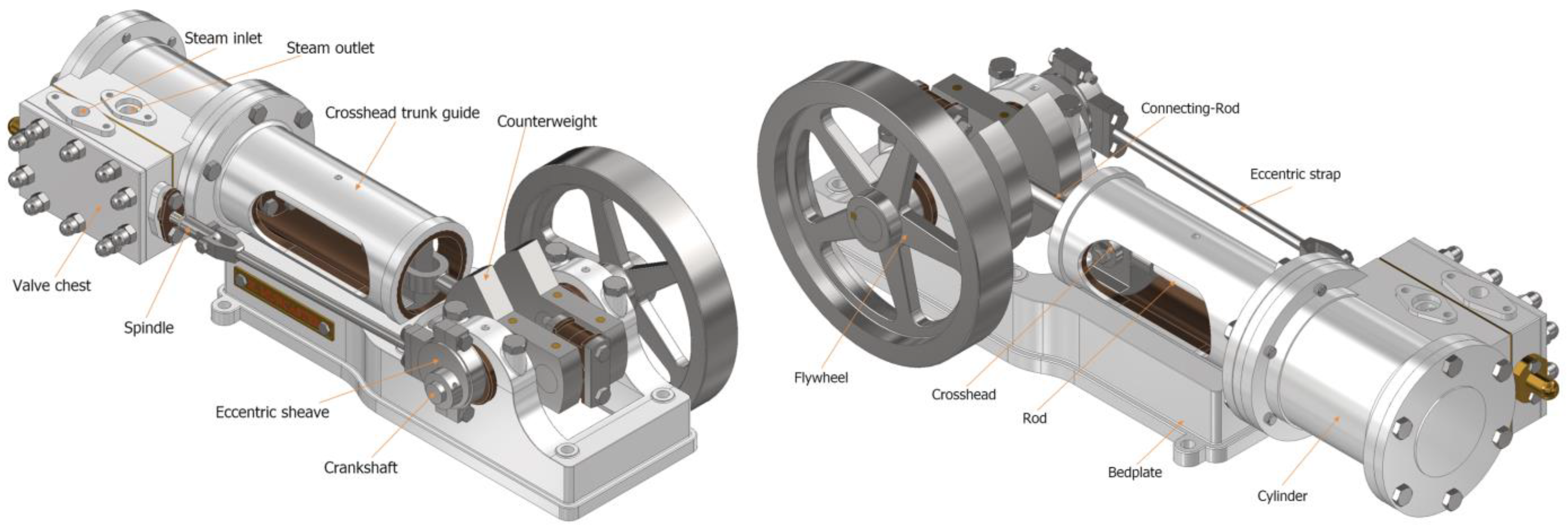
Figure 1 shows two images, the front and rear views of the final assembly of the invention, indicating the most notable elements.
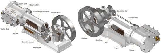
Figure 1.
Assembly of the machine: front view (left) and rear view (right).
This device comprises a single double-acting cylinder, indicating that the working fluid vapor (steam) enters and exits from both sides of the piston, executing two simultaneous thermodynamic cycles, albeit with a time differential. Specifically, while steam intake (steam inlet) transpires on one side of the piston, steam exhaust (steam outlet) occurs on the other side. Control over the intake and exhaust is administered by a slide valve situated within the valve chest block, adjacent to the cylinder. The motion of this slide valve is achieved via a coupling, facilitating relative movement between the components, made possible by the connection between the spindle of the slide valve and the crankshaft. Furthermore, an eccentric sheave is incorporated to synchronize the motion of the piston with that of the slide valve, ensuring that the intake and exhaust of steam transpire during specific intervals, thereby guaranteeing the optimal operation of the machine.
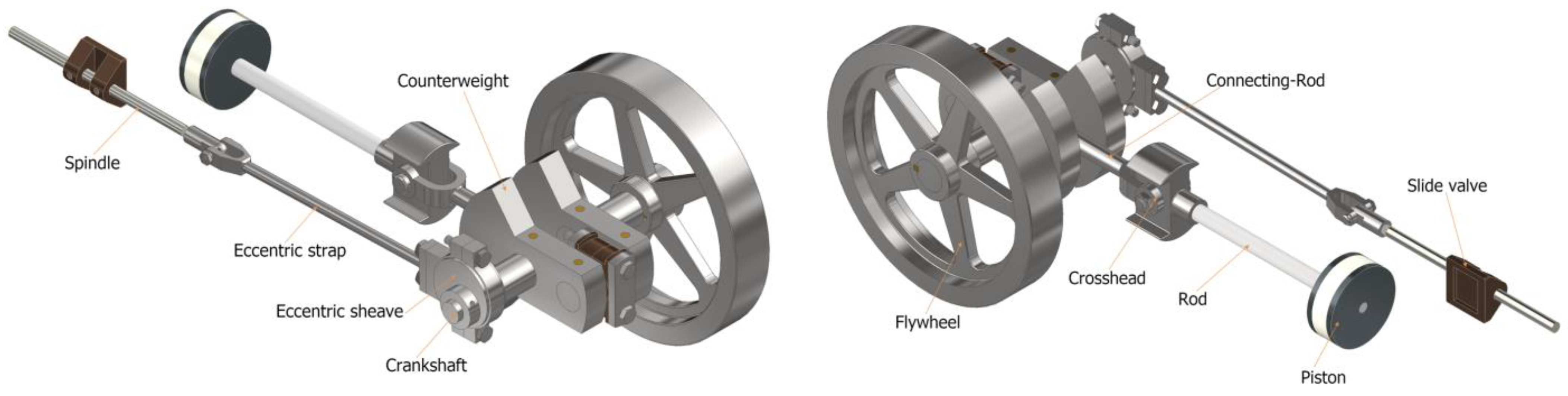
A noteworthy feature of the machine and its design is the sub-assembly of the moving components, particularly the crosshead, employed to convert the reciprocating motion of the piston into a rotary motion of the crankshaft (Figure 2).
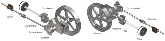
Figure 2.
Moving components: front view (left) and rear view (right).
Giving greater consideration to the steam intake and exhaust, it is worth noting that the reciprocating motion of the slide valve is driven by the eccentric sheave, which rotates at the identical angular velocity as the crankshaft.
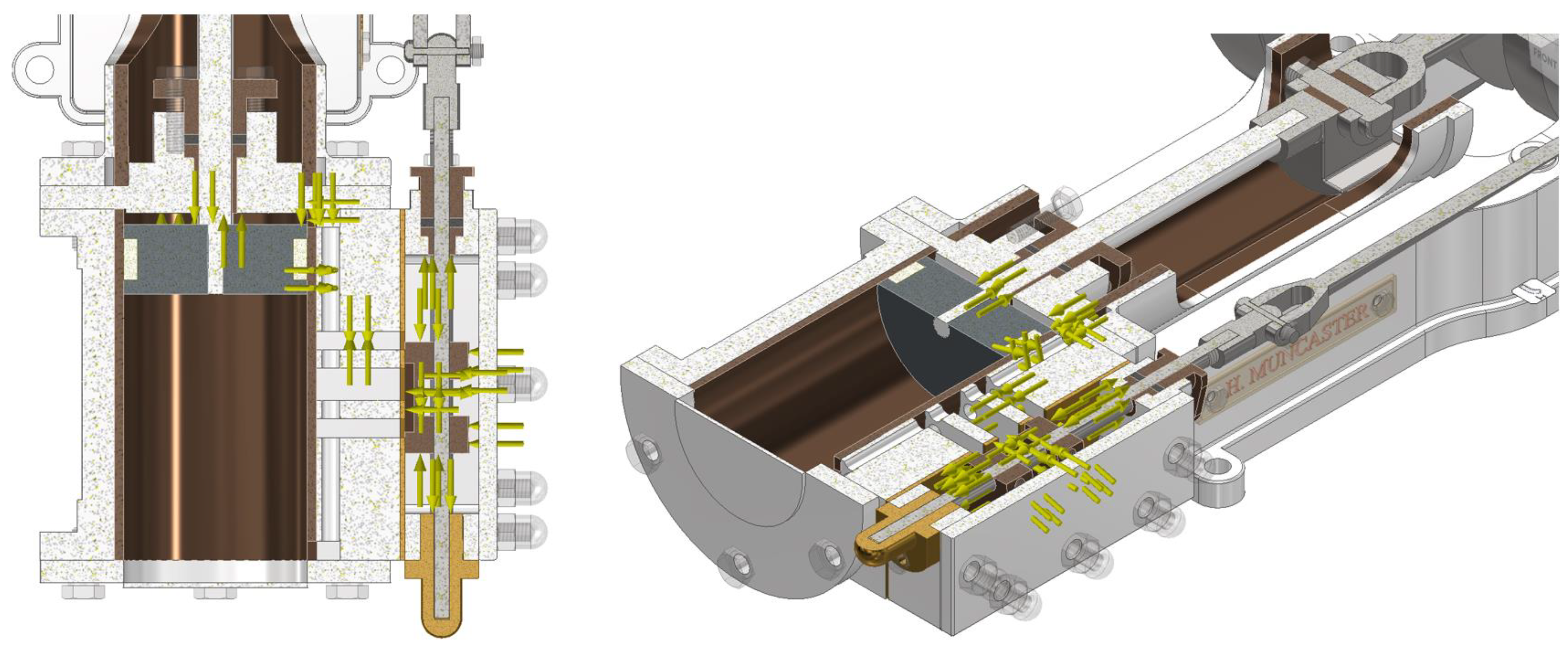
Figure 3 displays the axonometric and top views of the invention in sectional form, facilitating a clearer observation of the engine’s components, as well as the interior of the cylinder chamber and the valve chest.
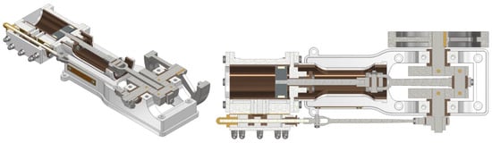
Figure 3.
Sectioned views of the assembly: axonometric view (left) and top view (right).
2.2. Analysis from the Mechanical Engineering Standpoint
This section elucidates each stage involved in conducting a linear static analysis utilizing FEM, along with the established operational assumptions. The numerical model employed is a linear three-dimensional contact finite-element model, which has undergone several stages. These stages encompass:
- Preprocessing
- Material Assignment
- Application of Contacts
- Boundary Conditions
- Discretization (Meshing)
- Identification of critical positions, determination of the deformation envelope, and execution of modal analysis and linear static analysis.
2.2.1. Preprocessing
An analysis encompassing the entire steam engine could indeed be conducted; however, due to the substantial number of components comprising it, the computational cost and simulation time would be prohibitively high. Consequently, elements that were not anticipated to significantly influence the obtained results were excluded from the analysis, particularly those operating under non-critical conditions.
In this study, joining elements were omitted, as many of them necessitate a very fine mesh and, moreover, their quantity within the assembly is substantial. Consequently, some of these elements (such as cap screws and nuts) were substituted with a “bonded”-type contact relationship, simulating a welded joint. Nonetheless, it is crucial to note that a welded joint is inherently more rigid than a joint utilizing cap screws and nuts. Therefore, if critical stress values arise in an area where a joining element ought to be present or in the contact region, these initially excluded elements must be reintegrated.
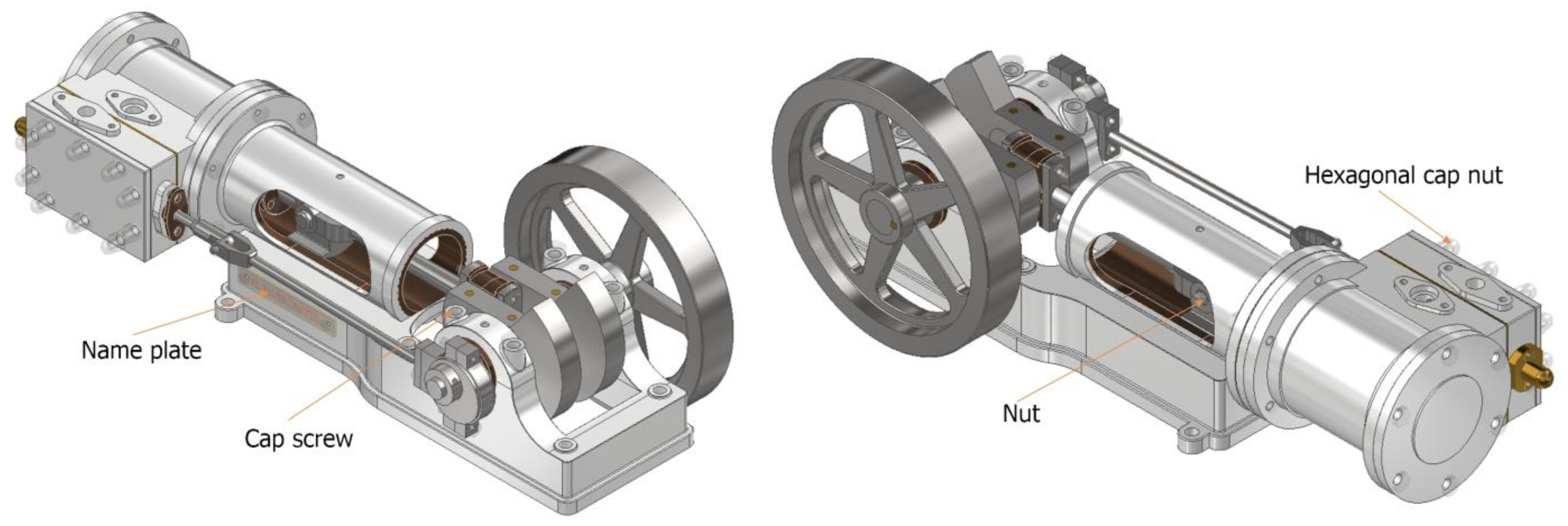
Figure 4 illustrates the simplified assembly upon which the linear static analysis was based, highlighting some of the components that were excluded from the analysis.
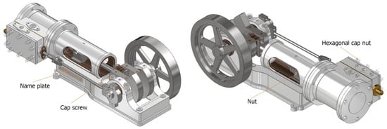
Figure 4.
Isometric view of the simplified assembly: front view (left) and rear view (right).
2.2.2. Assignment of Materials
During this stage, materials were assigned to each component of the 3D CAD model to endow the solid with the mechanical properties inherent in the chosen material. The material selection significantly influences the behavior of the elements. For this investigation, materials were allocated from the Autodesk Inventor Professional 2024 materials library. Table 1 presents the materials along with their respective mechanical properties that were pertinent to the analysis.

Table 1.
Properties of each material used in the analysis.
2.2.3. Application of Contacts
For an accurate simulation using FEM, it is imperative to establish the existing contacts between the elements constituting the assembly. Autodesk Inventor Professional 2024 facilitates the automatic establishment of these contacts, offering significant advantages for assemblies comprising a large number of components. The manual establishment of contacts in such cases would be excessively time-consuming due to the high number of contacts involved. The existing contacts in the software are briefly elucidated below:
- Fixed contact: This type of contact assumes that the contacting parts are fixed to each other and cannot move or deform relative to other parts. It is used to model rigid connections, such as bolts or welds.
- Sliding contact: This type of contact allows relative movement between the contacting parts only in a specific direction. It is useful for modeling situations where slippage is expected, such as in guides or rails.
- No penetration contact: This type of contact allows contact between the parts but prevents penetration between them. It is helpful for modeling situations where parts are in contact but cannot pass through each other, such as in nested assemblies or joints.
- Interference contact: This type of contact is used in situations where the contacting parts are allowed to penetrate each other.
- Bonded contact: This type of contact assumes that the parts in contact are joined together as if they were glued. It is useful for modeling situations where parts are joined, such as with adhesives or welded joints.
- Pressure contact: This type of contact is for the contact between surfaces under a certain pressure but without friction. It is used to analyze situations where the pressure between the parts is relevant, such as gaskets or seals.
- Separation contact: This type of contact is for situations where the contacting parts can separate during analysis, that is, a gap is allowed to exist between the contacting surfaces. When a separation contact is used, the parts are allowed to move apart from each other if the forces applied exceed a certain threshold. This is useful for modeling situations where parts are expected to separate, such as the opening of a crack or the separation of components.
Within each contact type, the choice between symmetrical or asymmetrical contact is available. In symmetric penetration, the nodes of one mesh cannot penetrate the nodes of an adjacent mesh; in the asymmetric type, such penetration is permitted.
An inherent drawback associated with automatic contact generation is that the software exclusively creates them as bonded-type contacts. Consequently, the behavior of this model may not accurately reflect that of the real model, as there exist different types of contacts within the assembly.
To address this issue, we can choose between two options: enter all the contacts manually, which is not recommended given the complexity and number of elements of the assembly, or enter all the automatic contacts of a single type (of which it is thought that there are more, in this case the “bonded” type) and later change those that are not for the correct type of contact.
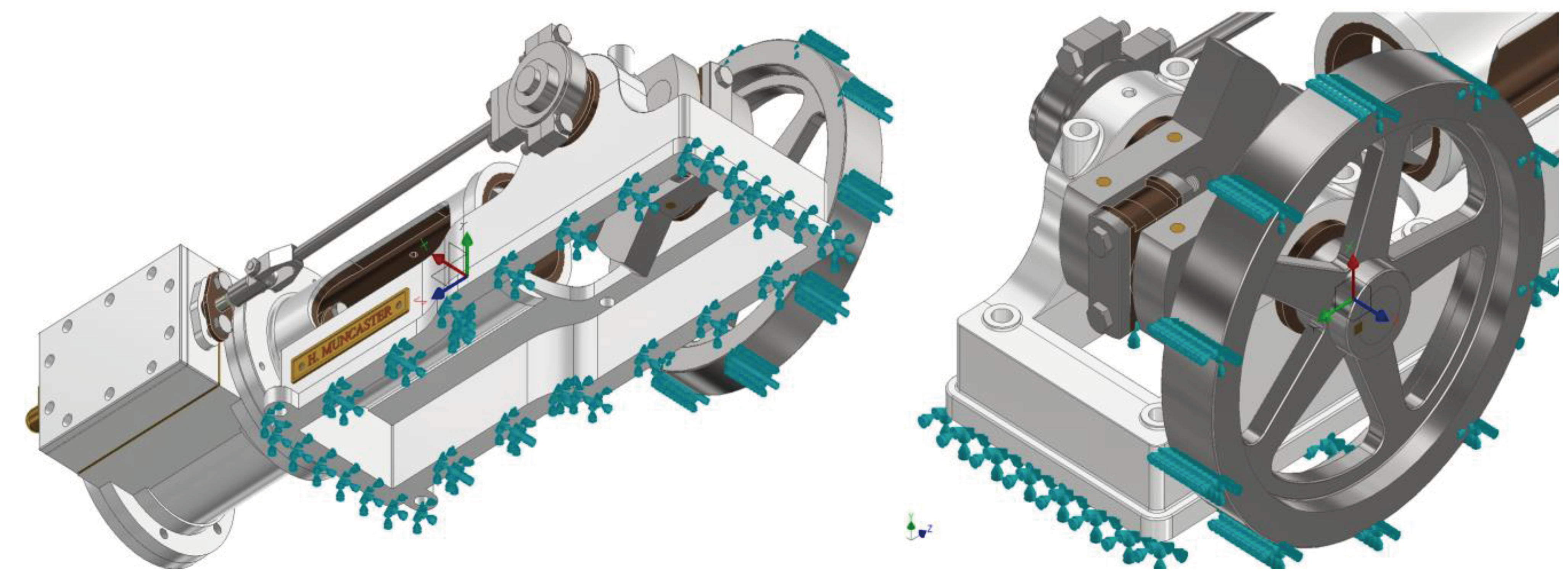
2.2.4. Boundary Conditions
Boundary conditions were imposed by constraining the six degrees of freedom of the lower surface of the bedplate and the flywheel (Figure 5). Concerning the lower surface of the bedplate (Figure 5, left), all displacements and rotations were constrained to simulate the connection of the base to another solid. For the flywheel (Figure 5, right), the external surface was restricted to simulate critical positions, such as the locking of the flywheel during the initiation of machine operation. The flywheel was immobilized (all degrees of freedom were restricted) as it is the sole means to transmit torque to the engine. To summarize, in both cases, displacements in all directions and rotations around the axis of the local reference system of each solid were restricted.
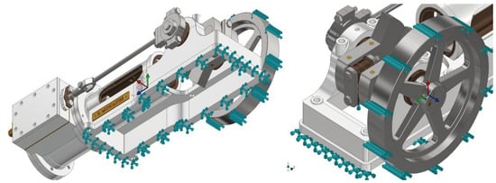
Figure 5.
Bedplate fixing (left) and flywheel fixing (right).
2.2.5. Discretization
To proceed with the preliminary steps before analysis, it was crucial to perform the discretization of the model. This entailed dividing the model into multiple elements, each defined by nodes. Consequently, the analysis variables were computed at these nodes, with interpolation between them to determine the values within each element. The accuracy of this interpolation was contingent upon the number of nodes within each element; a higher number of nodes, corresponding to smaller element sizes, yielded a solution that more closely approximated reality. This aspect is crucial for the mesh quality, as these elements must be sufficiently small to capture the structural behavior’s details, yet not so small as to render the computational problem intractable. For a better understanding of this stage, a brief introduction is set out below.
The elements can be of various types, such as tetrahedral, hexahedral, or prismatic, contingent on the model geometry and the analysis requirements. Each element possesses a shape function that delineates the interpolation of displacements within the element from the nodal displacements. These shape functions are polynomials ensuring the continuity of displacements throughout the discretized domain.
Consequently, the governing differential equations of the system’s behavior were discretized into a system of algebraic equations derived through the application of the least squares principle or the Galerkin method. For each element, a stiffness matrix was constructed, which correlated nodal displacements with nodal forces. The global stiffness matrix of the system was then obtained by assembling the stiffness matrices of all individual elements [31].
Once the global stiffness matrix was assembled and the boundary conditions and loads were applied, the system of linear equations was solved. For linear static analysis, the system is:
where f represents the vector of applied forces, K denotes the global stiffness matrix, and u is the vector of unknown nodal displacements.
The results were then analyzed using post-processing software, which evaluates displacements, stresses, and strains within the model to ensure adherence to design and safety criteria. The equilibrium equations for a continuous system can be formulated as partial differential equations:
where σ represents the stress tensor and f denotes the applied force vector; it can be solved from the preceding equation. This is feasible because the global stiffness matrix K is derived by integrating the shape functions and material properties over the finite elements [32].
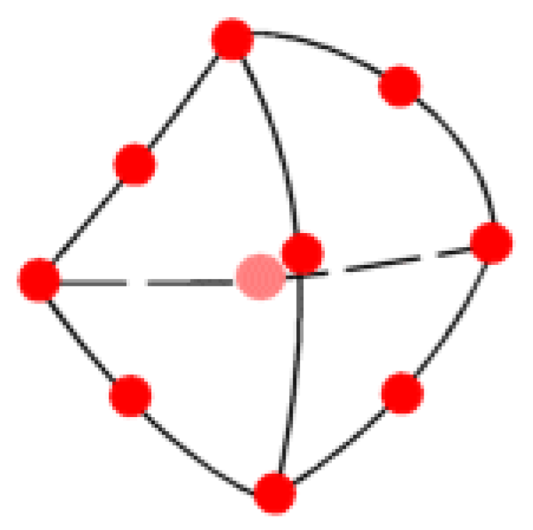
In this study, quadratic interpolation elements were used, specifically parabolic-type elements (tetrahedra) (Figure 6), to achieve results as close as possible to reality. The software automatically generates a coarser mesh in larger areas and a finer mesh in smaller areas, allowing the grid to better fit the geometry of the part and improving the accuracy of the results. An average element size of 0.0025 m, a maximum element growth ratio of 1.1, a maximum rotation angle of 65°, and a minimum element size of 0.001 m were defined. This configuration provided greater control over the mesh in contact areas. Following automatic meshing, the mesh was refined in specific areas where problems were anticipated, to facilitate a more precise study. In this research, the analysis was performed with a mesh consisting of 4,579,216 elements and 6,815,049 nodes.

Figure 6.
Parabolic-type element: tetrahedron.
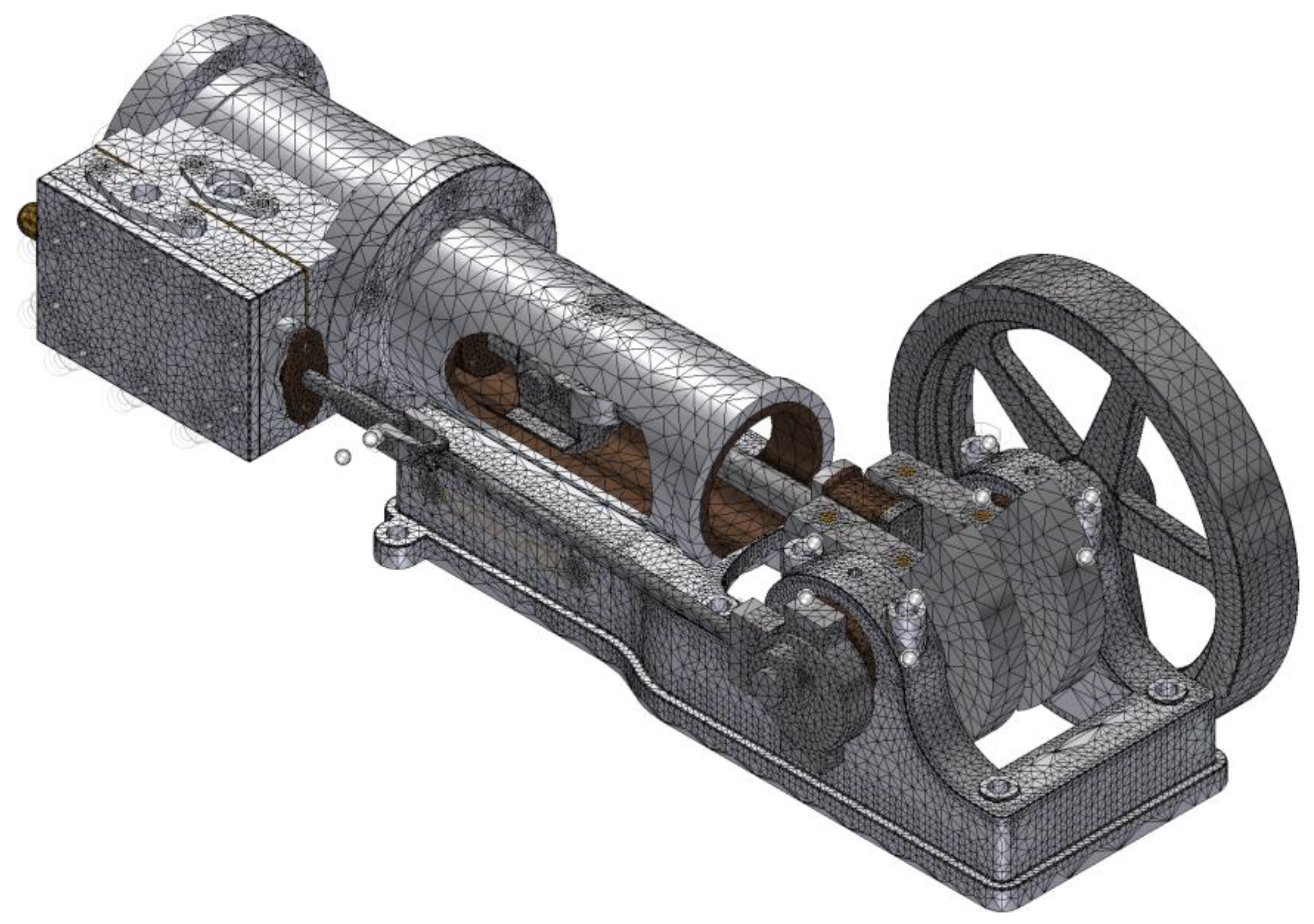
Following this brief overview of FEM and its relevance to the problem, we can observe the automatic discretization generated by the software (Figure 7).
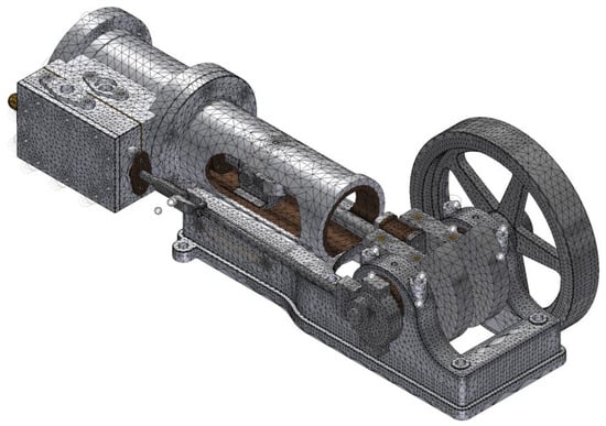
Figure 7.
Automatic mesh of the analysis.
2.2.6. Critical Positions
Analyzing critical engineering positions, such as those of a steam engine, is crucial to understanding how the system behaves under extreme conditions. In the case of a steam engine, two critical positions are normally considered: the lower dead center and the upper dead center after closing the steam inlet. These positions represent situations where the engine experiences maximum pressure differences across the piston, resulting in significant stresses and strains.
In a double-acting steam engine such as the one described, it is necessary to examine both situations because the pressure varies between the chambers as the steam is renewed and the exhaust occurs. In these critical positions, with one chamber experiencing maximum pressure and the other at atmospheric pressure, the stresses in the piston and cylinder chamber are most pronounced.
Thus, blocking the flywheel during the analysis allowed us to simulate the operation of the engine and analyze the transmission of force from the piston to the various components.
Figure 8 provides visual representations of the steam engine in both critical positions, highlighting the arrangement of the components, in particular the connecting rod, the piston rod, and the connection between the spindle of the sliding valve and the eccentric strap. Understanding these critical positions and their implications is essential to designing efficient steam engines.
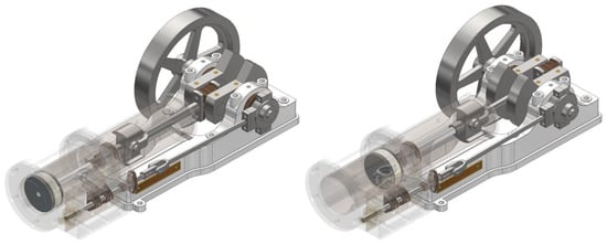
Figure 8.
Critical positions: lower dead center (left) and upper dead center (right).
2.2.7. Modal Analysis
A modal analysis in an assembly is a technique used in structural and mechanical engineering to understand the dynamic behavior of a system composed of multiple interconnected components. This type of analysis is performed in order to determine the natural frequencies and vibration modes of a system, which provides crucial information about its stability, response to dynamic loads, and potential resonance problems. Thus, if the natural frequencies are not zero and are also different, it could be verified that the assembly does not behave as a mechanism and a linear static analysis would be performed.
2.2.8. Linear Static Analysis
Once it has been confirmed that none of the natural frequencies of the vibration modes are equal to 0 Hz, a linear static analysis can be executed. For a better understanding of this stage, a brief introduction is set out below.
This analysis is based on several fundamental assumptions: linear elasticity, small deformations, and static equilibrium conditions. Hooke’s law states:
where is the stress, which is linearly proportional to the strain , with E being the material’s modulus of elasticity.
The assumption of small deformations implies that changes in the system’s geometry are negligible, thereby preserving the original configuration. Additionally, static equilibrium requires that the sum of all forces and moments acting on the system equals zero.
The equations governing linear static analysis involve equilibrium equations, stress–strain relationships, and strain compatibility. For a system in static equilibrium, internal forces must balance external forces. The stress–strain relationship is derived from the linear elastic behavior of materials, while compatibility conditions ensure that deformations conform to boundary conditions and interactions between different structural components [33].
The mathematical formulation for this scenario involves differential equilibrium equations for an axial load P and an internal pressure p acting on a differential element and other regions where the load is applied.
where N is the normal force, V is the shear force, M is the bending moment, and q is the distributed load.
Likewise, the strain–displacement relationships for axial deformation are given by:
where u is the axial displacement.
For bending deformation, the strain is:
where is the transverse displacement.
On the other hand, stress–strain relationships adhere to Hooke’s law for normal and shear stresses, which are defined by the following equations:
where is the shear modulus and is the shear strain [34].
Finally, by solving these differential equations, taking into account the boundary conditions and applied loads, the displacements and stresses at each point are obtained.
To achieve the most accurate results, mesh convergence must be performed until the maximum von Mises stress value stabilizes and shows minimal variation.
Additionally, accurately determining the stress envelope is crucial to ensure a correct analysis and to avoid erroneous results.
Steam conditions at the cylinder inlet vary depending on the geometry of the machine, as well as the dimensions of the piston and chamber, and its intended application. The working pressure to be obtained is the highest possible; this can be achieved by increasing the number of molecules, by increasing the steam temperature, and, finally, by reducing the space, that is, by reducing the diameter of the cylinder.
Despite the absolute absence of precise machine operating data, an initial simulation was carried out assuming a gauge working pressure of 0.62 MPa (data received from real examples of steam engines in locomotives) [35], which is equivalent to a force of 800 kg for a piston of 0.040 m diameter. This pressure was applied to various components, including the slide valve block and piston face, depending on their positions. On the other hand, the gauge pressure chosen took into account the atmospheric pressure in the opposite chamber. Thus, as the steam expanded, the exhaust valve opened, releasing steam at atmospheric pressure, while steam at working pressure was admitted into the other chamber. This type of engine with this small size was not usually used in isolation, but, for example, in a locomotive, two engines were used on each side, increasing its efficiency until reaching a force of 58,000 kg by using larger-diameter pistons.
Subsequently, after applying a gauge working pressure of 0.62 MPa, the machine’s performance was evaluated. If the minimum safety factor was found to be less than unity, indicating that the yield strength was exceeded, the steam engine failed under the static load of the first cycle. Therefore, iterative analyses were required to identify a pressure level that ensured the maximum von Mises stress remained below the yield strength and the safety factor exceeded unity, ensuring safe operation.
Thus, it was a question of defining the range of manometric working pressures that provided safety factors, for both critical positions, that were as close as possible to the values of 2 and 4, given that, in the design of modern machines, this is their optimal range. After the simulations were carried out, it was verified that the most restrictive position to obtain the maximum working pressure (0.320 MPa) was that of the upper dead center, obtaining a safety factor closest to 2. However, to obtain the minimum working pressure so that the safety factor did not exceed the value of 4, the most restrictive position was that of the lower dead center, with the pressure being 0.165 MPa.
However, this study focused more on the results that corresponded to those of the maximum admissible pressure (0.320 MPa) since, with this value, the maximum possible efficiency was obtained, although they were also verified for the minimum admissible pressure value (0.165 MPa).
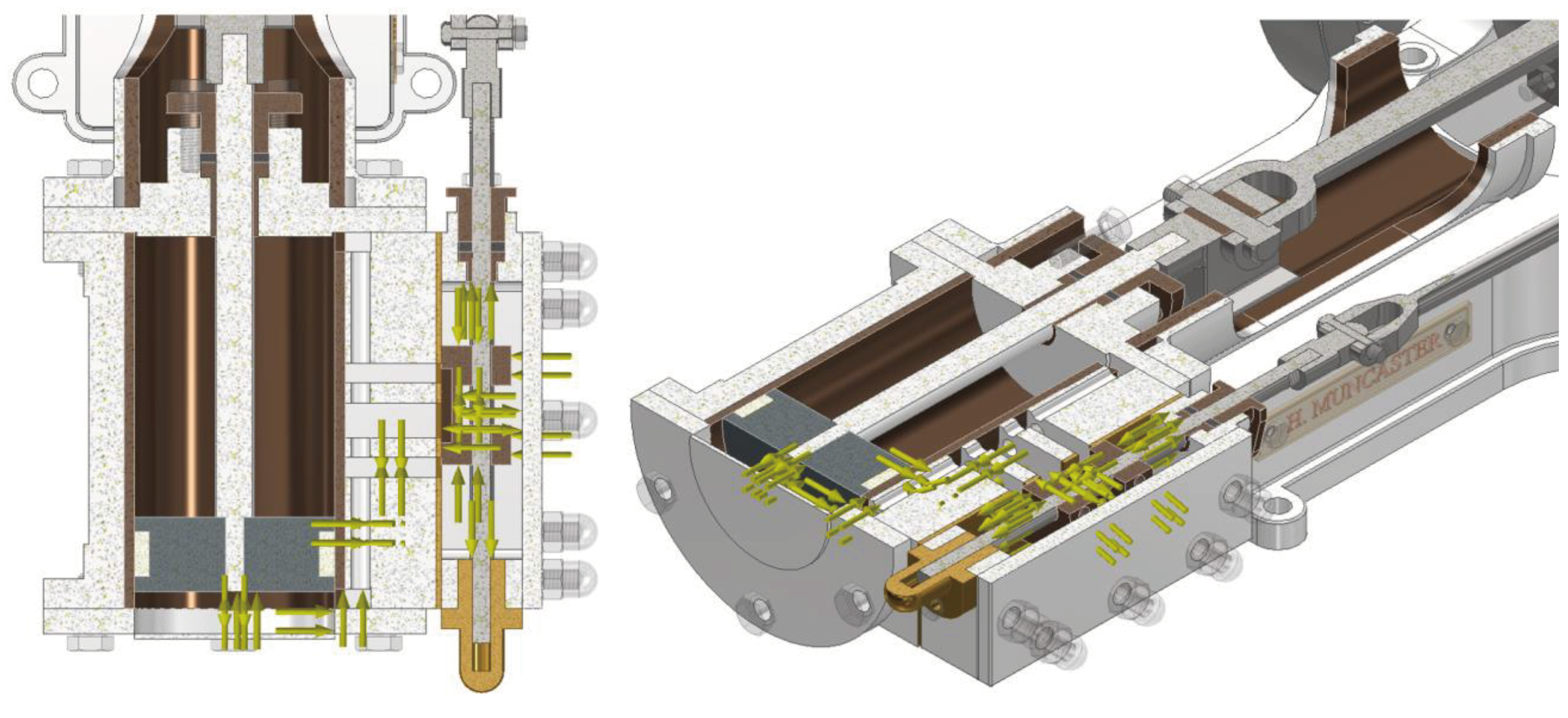
In Figure 9, we can see the application of pressure loads when the motor is at lower dead center.
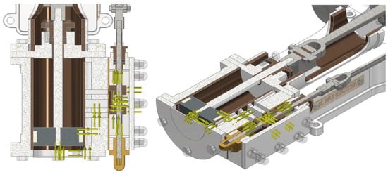
Figure 9.
Pressure loads at the lower dead center: top view (left) and axonometric view (right).
This process was similarly conducted at the upper dead center (Figure 10). In this instance, the pressure loads were applied to the opposite face of the piston and the upper part of the cylinder. This methodology allowed for the examination of both critical positions: one functioning under compression (lower dead center) and the other functioning in traction (upper dead center).
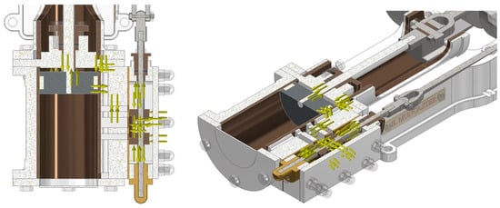
Figure 10.
Pressure loads at the upper dead center: top view (left) and axonometric view (right).
After applying the pressure loads, a linear static analysis was conducted. This was followed by generating a convergence analysis graph alongside the steam engine’s response, characterized by the von Mises stress values, displacement, and safety factor.
To ensure the reliability of the results, a manual mesh convergence analysis was performed due to the steam engine’s numerous components, which create a complex mesh. This manual analysis started with an initial discretization using a predetermined global size, followed by a simulation. The location of the maximum von Mises stress, the corresponding stress value, the element size, the relative error percentage, and the iteration number were identified.
Subsequently, a local mesh refinement was performed in regions with high stress concentrations by reducing the size of the finite elements. This refinement can involve vertices, edges, surfaces, or solids. In this instance, the connection between the piston rod and the connecting rod, specifically in the crosshead, was fully refined as this was where the maximum stresses were concentrated (Figure 11). After reducing the element size, the assembly was re-discretized and the simulation was iterated until the relative error in the von Mises stress values between consecutive iterations fell below a predefined threshold, specifically 10%.
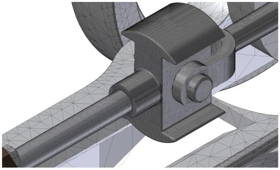
Figure 11.
Local mesh refinement.
3. Results and Discussion
3.1. Lower Dead Center
3.1.1. Modal Analysis
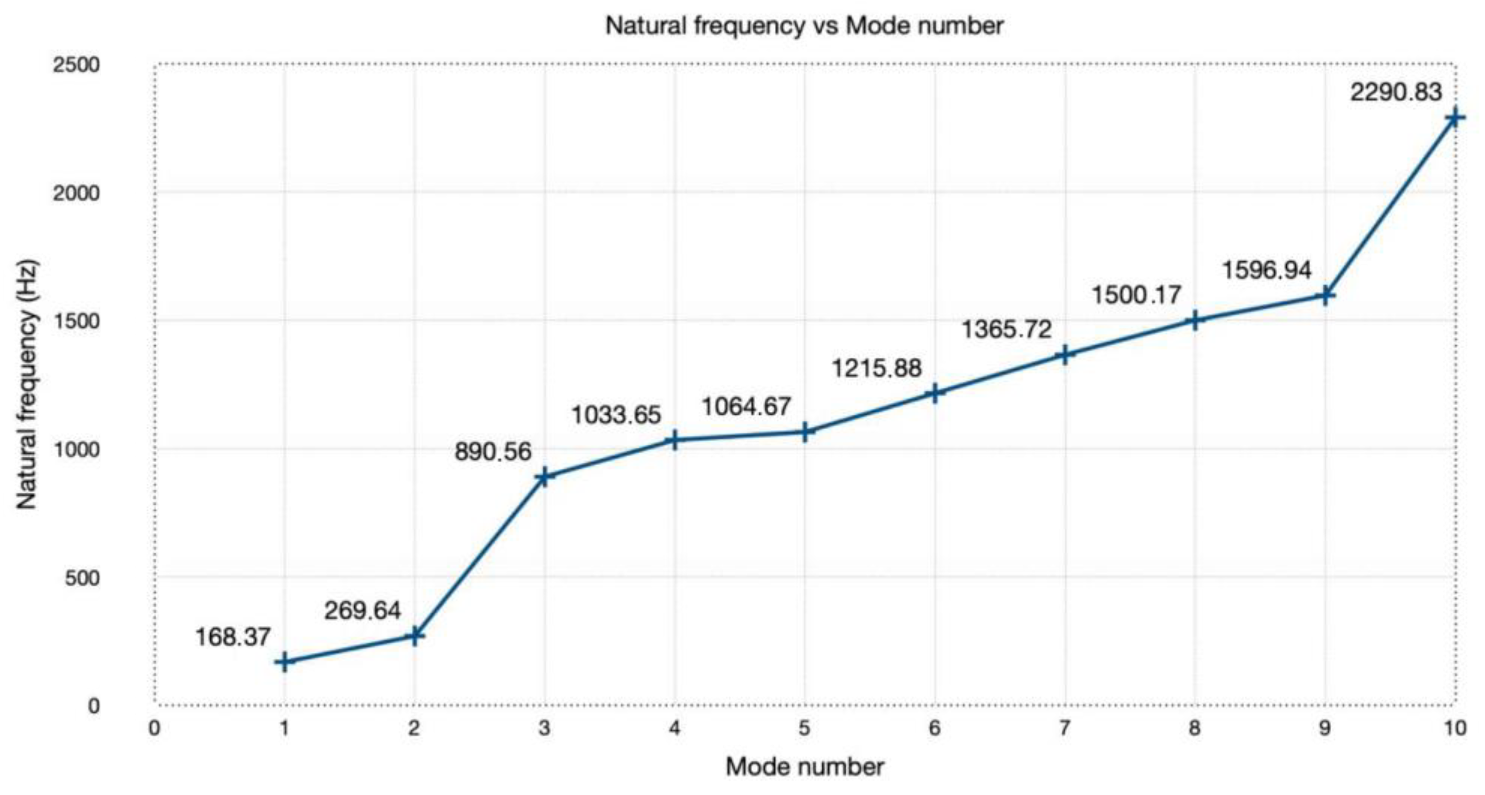
After imposing the appropriate boundary conditions, the simulation was carried out. Figure 12 presents a graph where the x-axis represents the vibration mode number and the y-axis denotes the natural frequency (Hz) corresponding to each vibration mode.
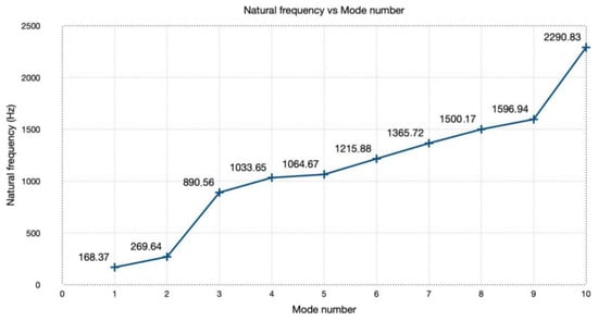
Figure 12.
Natural frequency vs. mode number.
The graph illustrates that vibration mode 1 had a frequency value exceeding 100 Hz, which was the lowest among its natural vibration frequencies. Consequently, as no natural frequency was zero, a linear static analysis was feasible under the given simulation conditions at the piston’s lower dead center position, ensuring that it would not behave like a mechanism.
3.1.2. Linear Static Analysis
Herein, we present the findings related to the critical position of the lower dead center, following the closure of the steam inlet to the cylinder, leading to its subsequent expansion within the chamber.
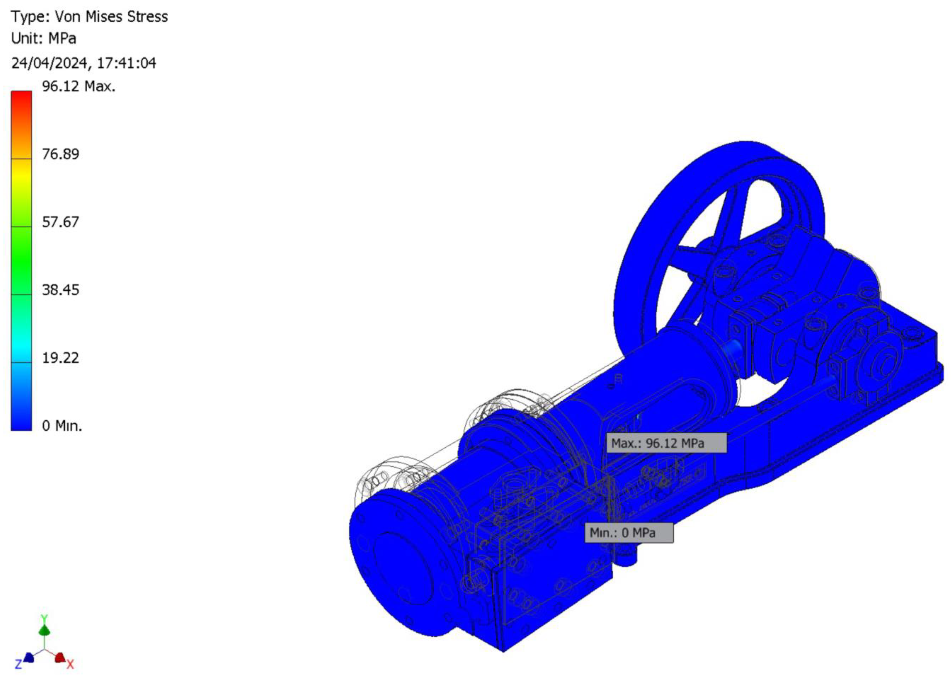
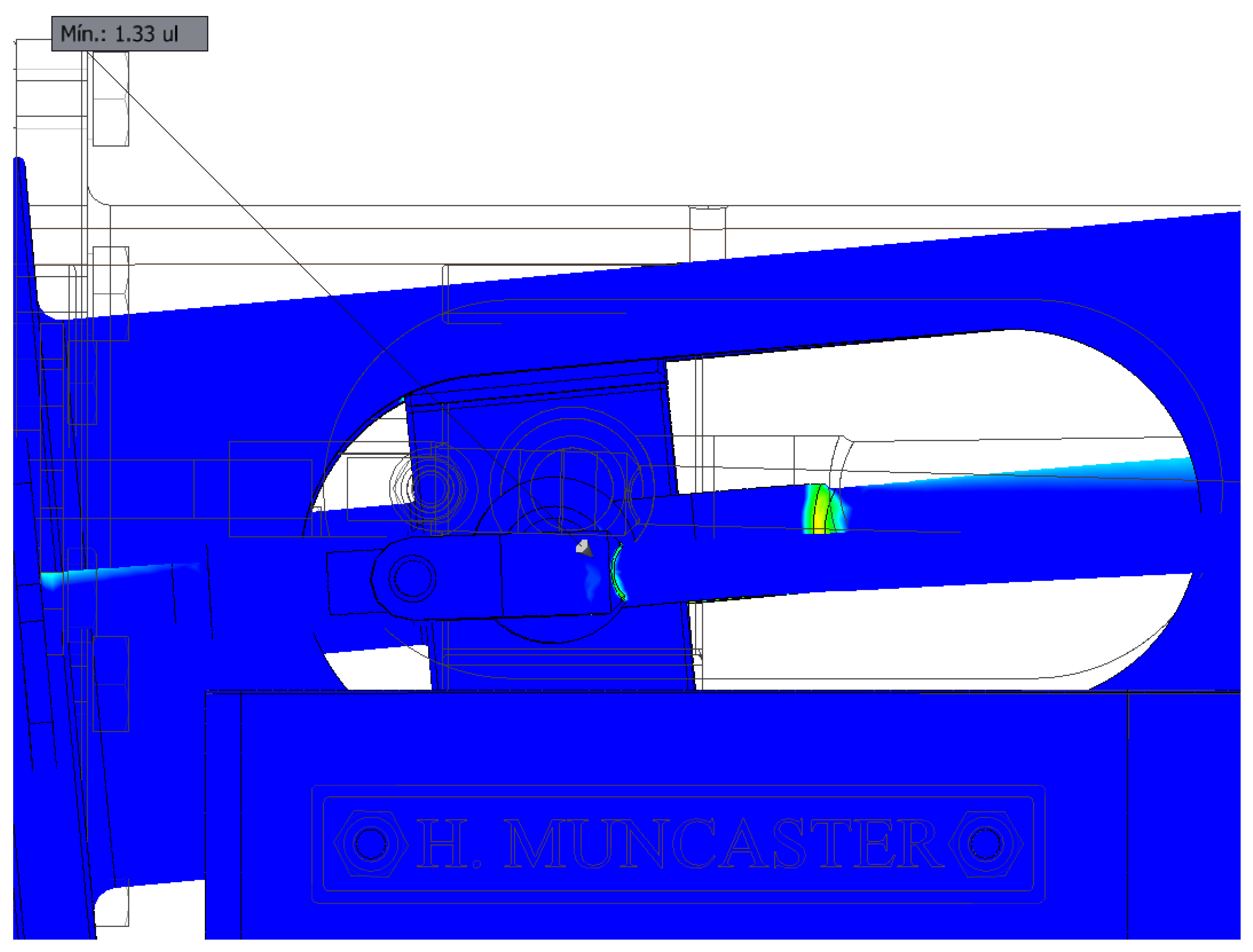
As previously discussed, an initial linear static analysis was conducted under a gauge working pressure of 0.62 MPa, yielding a maximum von Mises stress of 96.12 MPa (Figure 13) and a minimum safety factor of 1.33 (Figure 14), both located in the same region. As noted earlier, the safety factor must exceed unity, but for an optimal machine design, a recommended range between 2 and 4 is advised to ensure reliable operation.

Figure 13.
Maximum von Mises stress for a pressure of 0.62 MPa.
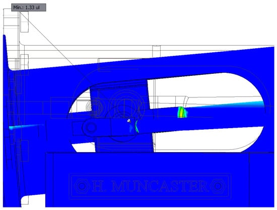
Figure 14.
Minimum safety factor for a pressure of 0.62 MPa.
Thus, it can be inferred that the machine would not fail at a steam inlet pressure of 0.62 MPa. However, to optimize this value towards a safety factor of 2, a subsequent analysis was required with a reduced working pressure, specifically 0.32 MPa. The objective was to evaluate if this pressure ensured the machine’s proper functioning.
Through these simulations, the location with the lowest safety factor was identified to refine the mesh accordingly. In this case, it was determined that this critical point was at the junction between the piston rod and the connecting rod.
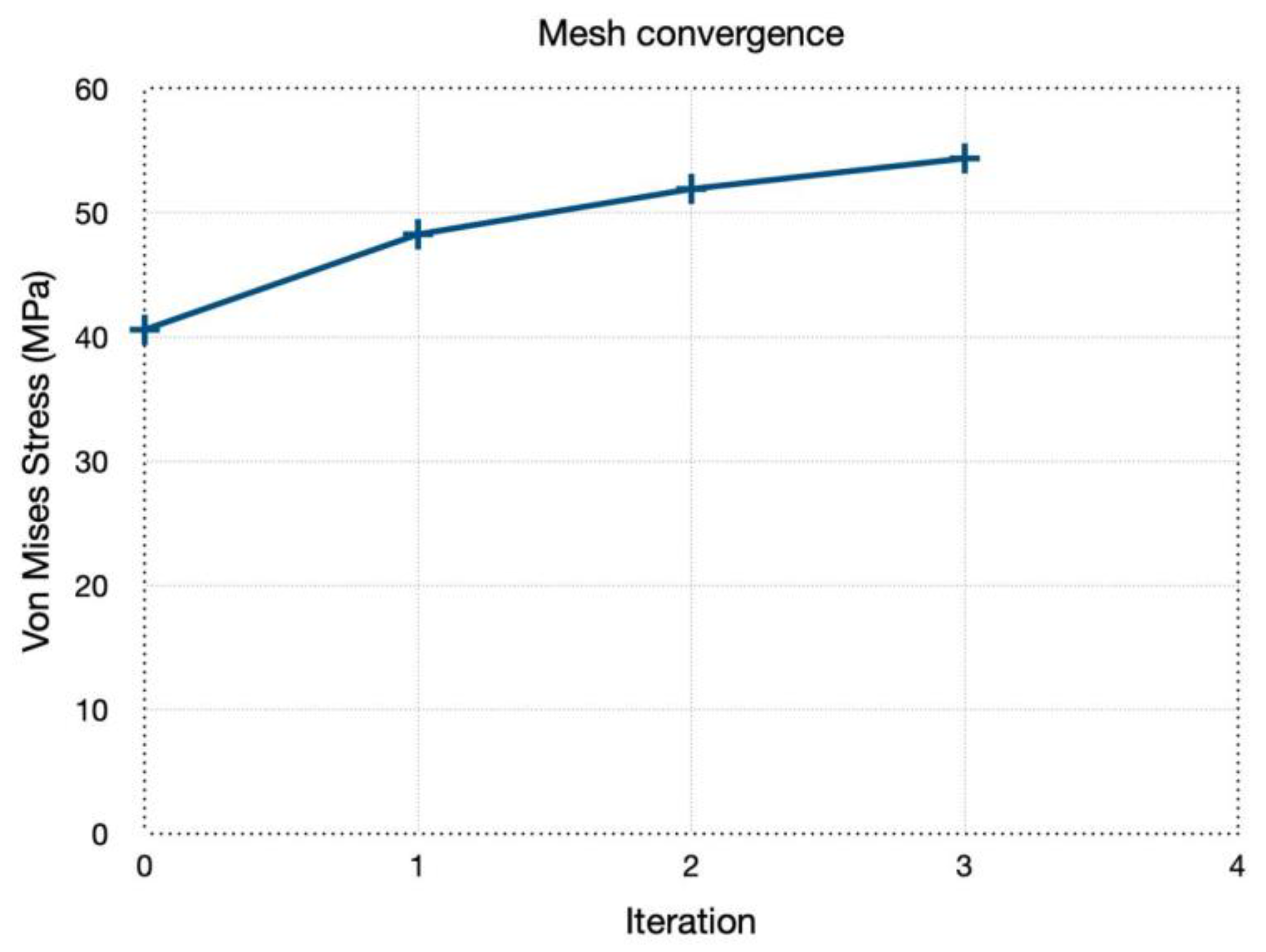
After carrying out the analysis with various mesh element sizes in the piston rod and connecting rod, the mesh convergence analysis graph was obtained (Figure 15). Additionally, data on the element size, von Mises stress, relative error percentage, and iteration number are summarized in Table 2.
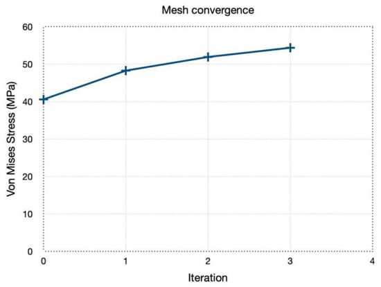
Figure 15.
Mesh convergence graph.
Table 2.
Mesh convergence analysis.
In Table 2, it is demonstrated that mesh convergence was achieved with an element size of 5 mm, resulting in a relative error of 7.56% in the second iteration. However, further refinement was performed, reducing the relative error to 4.74% with an element size of 2.5 mm in the third iteration.
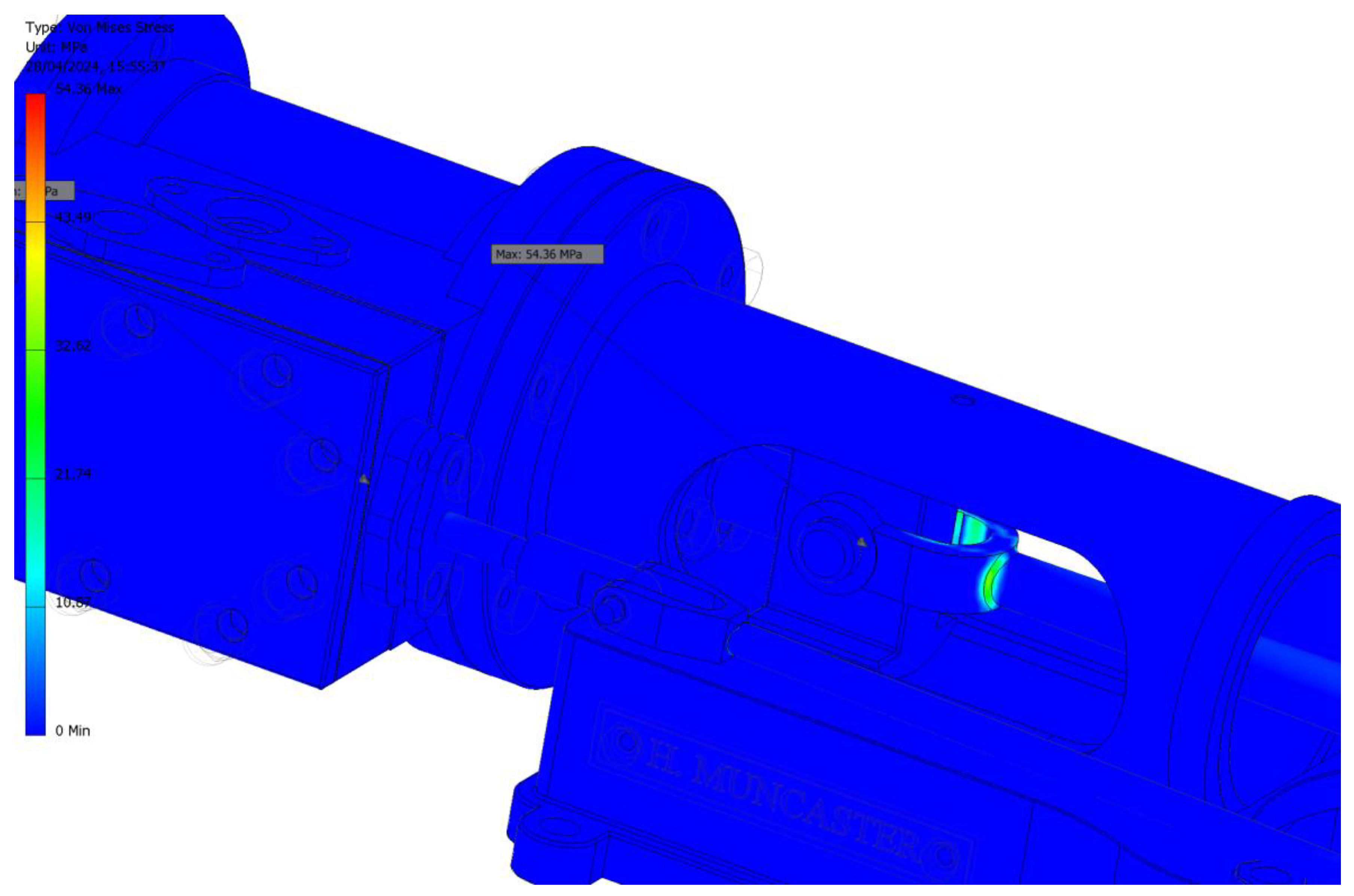
Furthermore, Figure 16 illustrates the distribution of von Mises stresses, while Figure 17 pinpoints the location of the maximum stress value, which was specifically at the junction between the piston rod and the connecting rod, known as the crosshead.
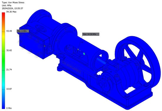
Figure 16.
Von Mises stress distribution.
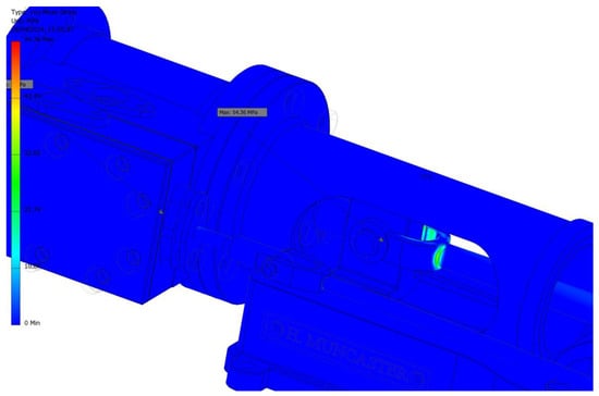
Figure 17.
Location of the highest value of von Mises stress.
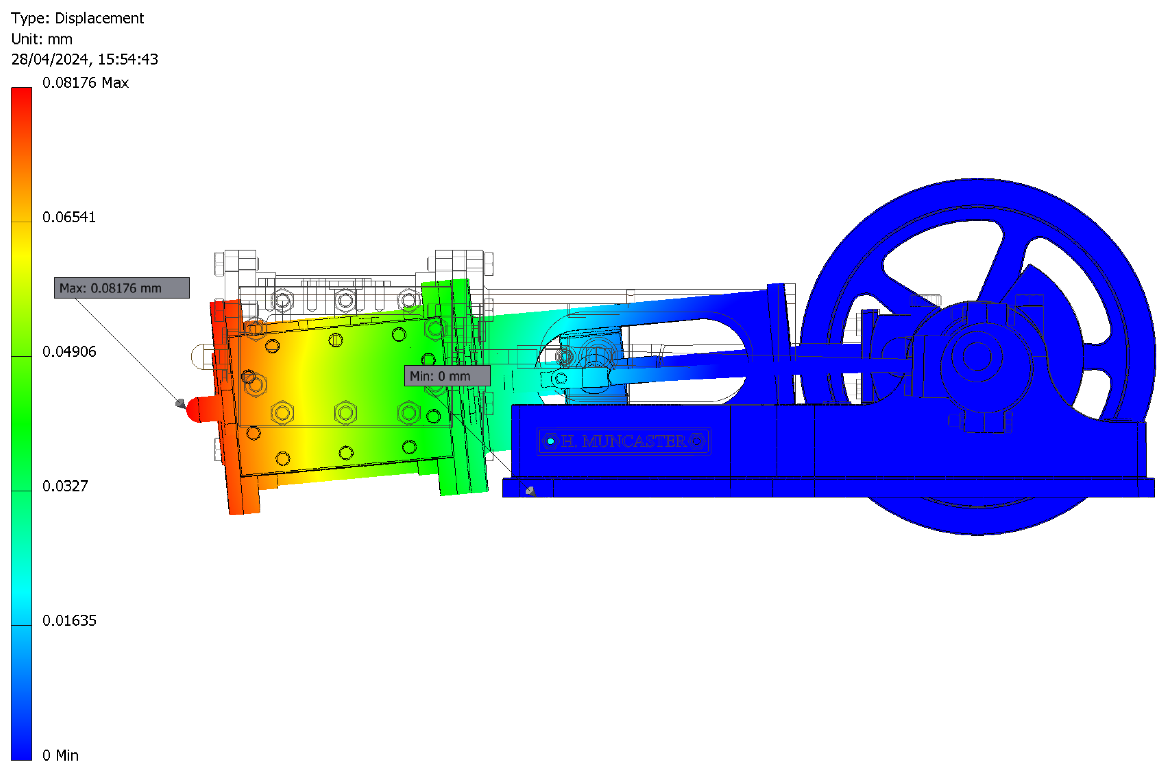
Similarly, the distribution of displacements was obtained (Figure 18) and is shown with an increased scale factor (×2) for better observation. As can be seen, the value was negligible, but it was considered since it was the only part of the engine that was cantilevered.

Figure 18.
Displacement distribution with a ×2 scale factor.
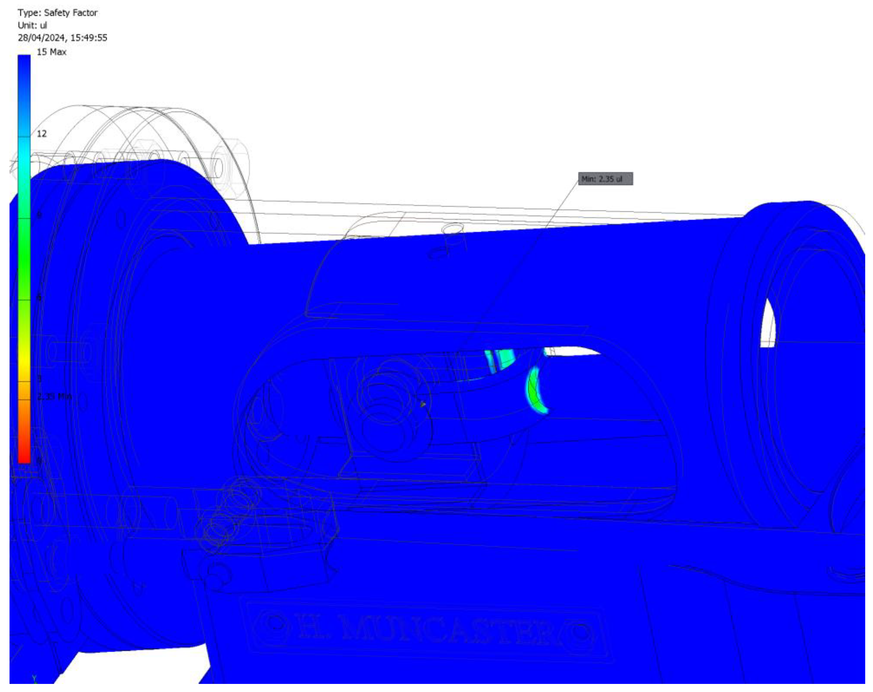
Finally, Figure 19 shows the distribution of the safety factor, and Figure 20 shows the location of its minimum value (2.35).
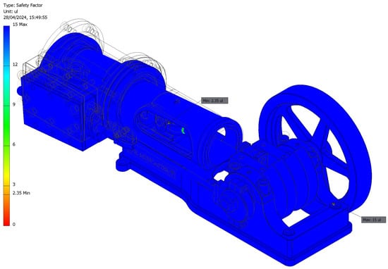
Figure 19.
Safety factor distribution.

Figure 20.
Location of the minimum safety factor.
3.2. Upper Dead Center
3.2.1. Modal Analysis
Figure 21 presents a graph depicting the modal analysis conducted for this critical position, analogous to the previously examined critical position. Notably, it was observed that none of the natural frequencies were zero, thereby justifying the application of linear static analysis. This indicates that under the simulation conditions at the critical position corresponding to the piston at the upper dead center, the system did not exhibit the behavior characteristic of a mechanism.
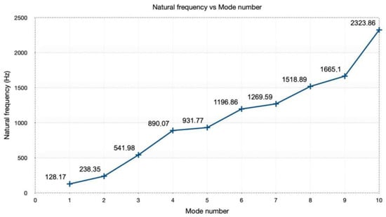
Figure 21.
Natural frequency vs. mode number.
3.2.2. Linear Static Analysis
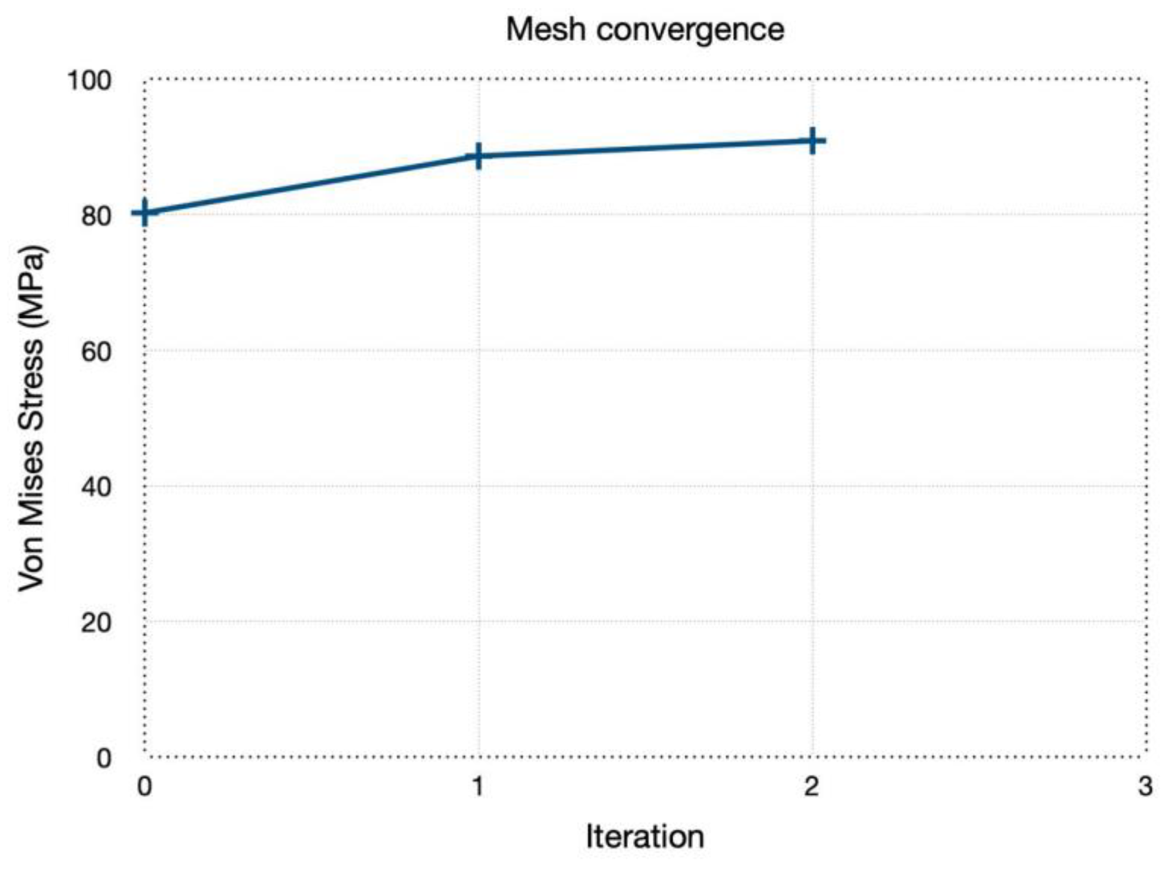
Similar to the analysis at the lower dead center, the working pressure was set at 0.32 MPa. It was imperative to verify whether all the values conformed to the required criteria, with particular attention to ensuring the safety factor exceeded unity. Upon conducting the analysis with various mesh sizes, a mesh convergence analysis graph was generated (Figure 22). Additionally, data regarding element size, von Mises stress, relative error (%), and iteration number were compiled (Table 3).
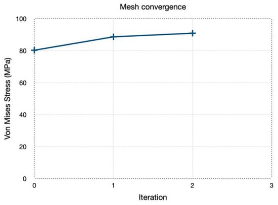
Figure 22.
Mesh convergence graph.
Table 3.
Mesh convergence analysis.
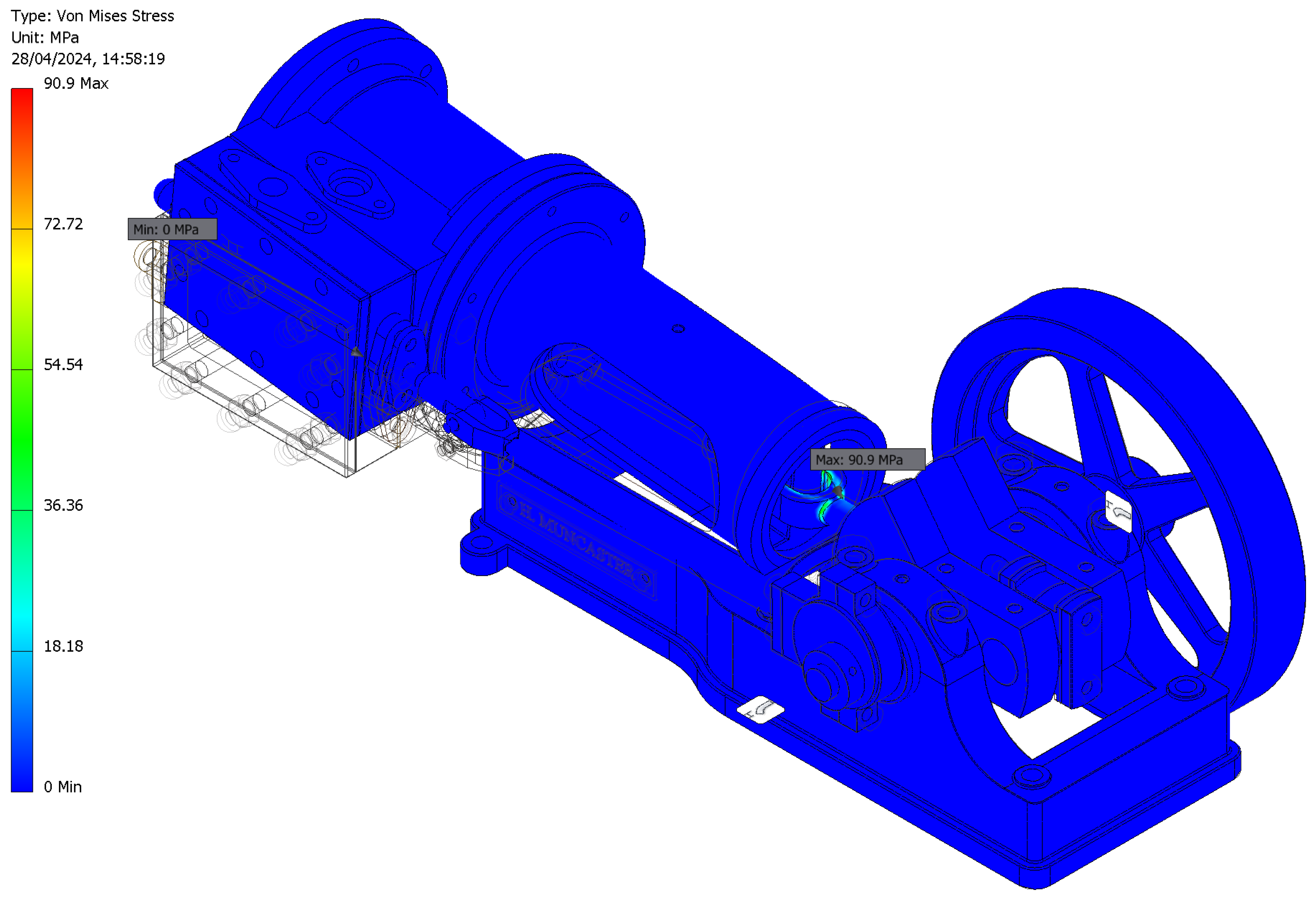
The data presented in this table indicate that the relative error for an element size of 2.50 mm was 2.55% during the second iteration. This value fell within an acceptable range, affirming the accuracy of the analysis results. Figure 23 illustrates the von Mises stress distribution, while Figure 24 highlights the specific location of its maximum value, situated in the connecting rod.

Figure 23.
Von Mises stress distribution.
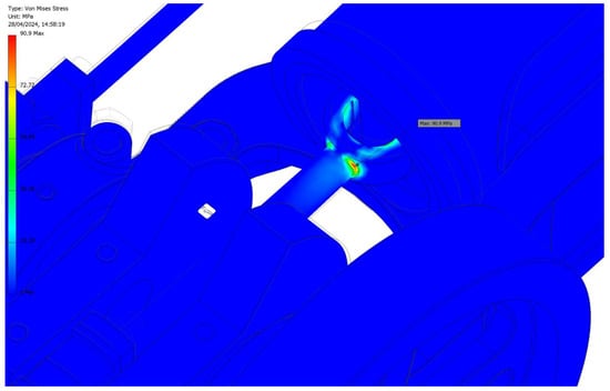
Figure 24.
Location of the highest value of von Mises stress.
In addition, the distribution of displacements was obtained (Figure 25) and is shown with an increased scale factor (×2) for better observation. As can be seen, the value was negligible but it was considered since it was the only part of the engine that was cantilevered.
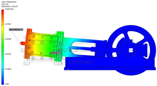
Figure 25.
Displacement distribution with a ×2 scale factor.
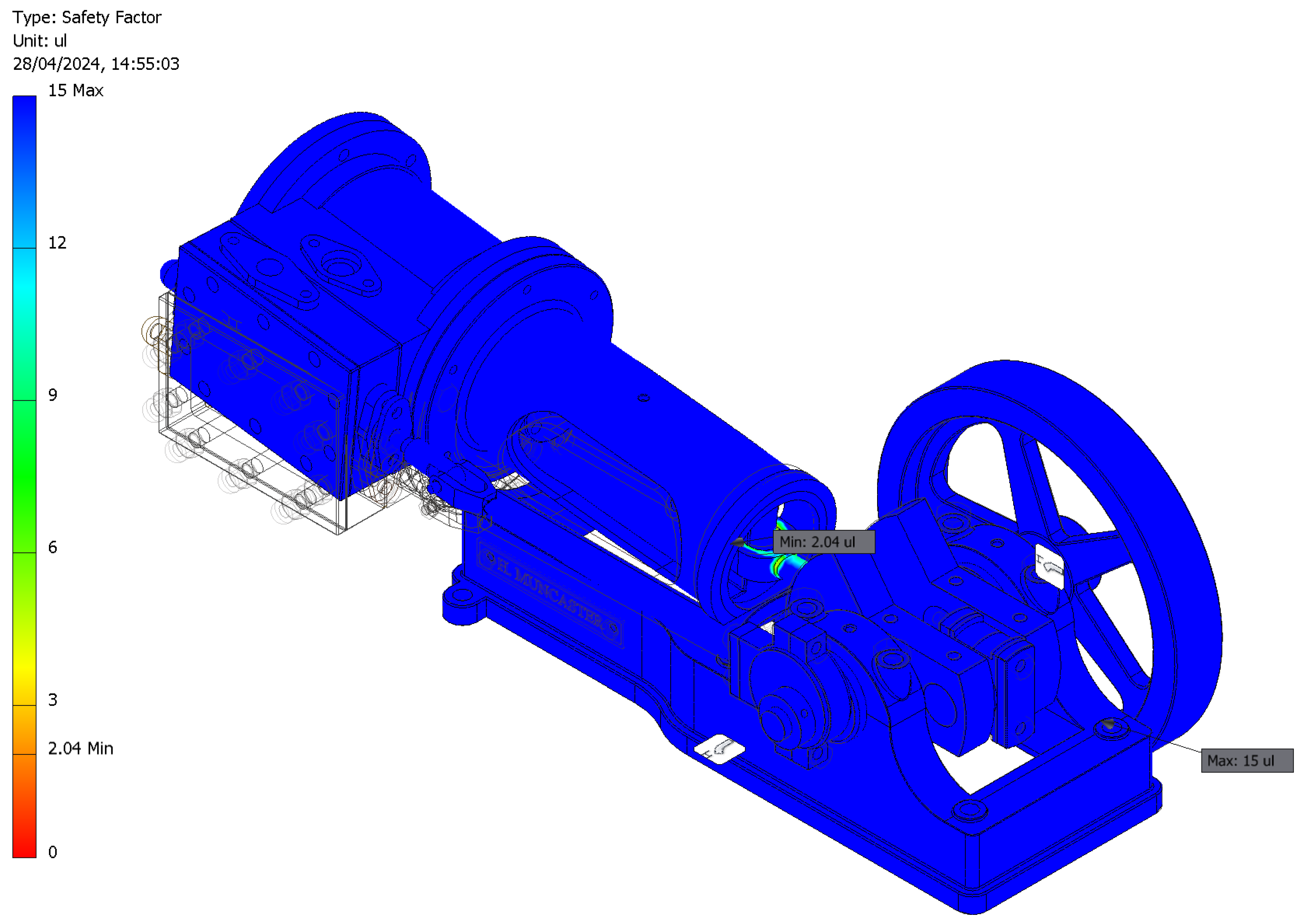
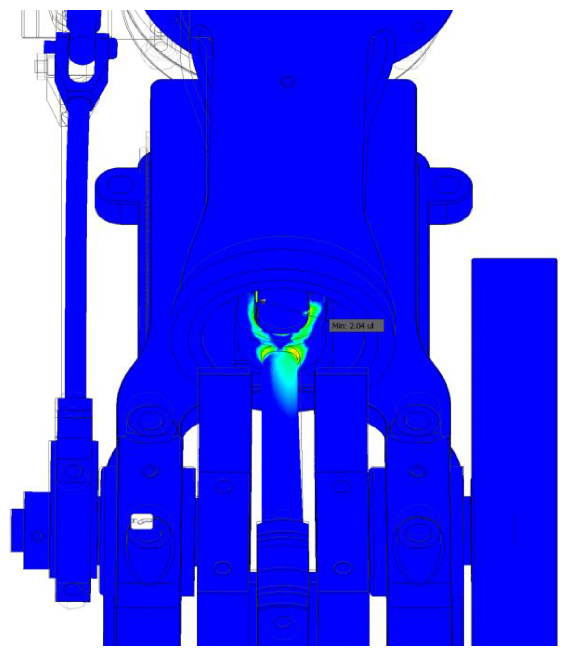
Finally, Figure 26 illustrates the distribution of the safety factor, and in Figure 27, the position of the lowest value (2.04) is shown, located in the connecting rod.

Figure 26.
Safety factor distribution.
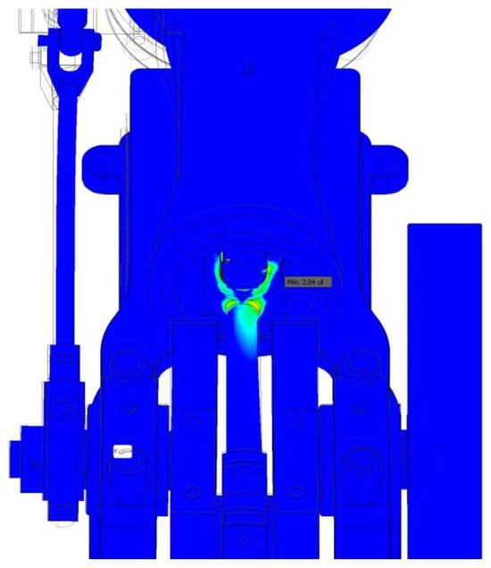
Figure 27.
Location of the minimum safety factor.
3.3. Discussion of the Results
The results indicate that the maximum von Mises stress is located at the top dead center position. Additionally, it was noted that a tensile load may induce buckling in the connection between the connecting rod and the piston rod. Future investigations could examine whether this connecting rod satisfies the buckling failure criterion.
Regarding displacements, a scale factor of 2 was employed to more clearly visualize the deformed configuration of the steam engine at both critical positions (lower and upper dead center). It is logical that the maximum displacements occur at the observed location, as that portion of the steam engine functions as a cantilever. This observation suggests that potential optimization could involve enhancing the bedplate design by extending it to the valve chest area and securing it with cap screws. Nonetheless, the observed displacements are negligible, which supports the efficient operation of the steam engine under the given pressure load. This validates the hypothesis of small deformations, allowing for calculations to be performed in the undeformed state using the Eulerian formulation method for discretization, thereby reducing computational costs. Furthermore, the absence of significant deformations ensures minimal friction due to the relative movement between components.
Moreover, the safety factor exceeds unity as intended and the optimal admissible steam pressure at the inlet (operating pressure) for this machine was identified as 0.320 MPa. This pressure ensures a safety factor within the range of 2 to 4. This value can be utilized to determine the operating pressure for other similar machines by relating the parameters of both models through dimensional analysis.
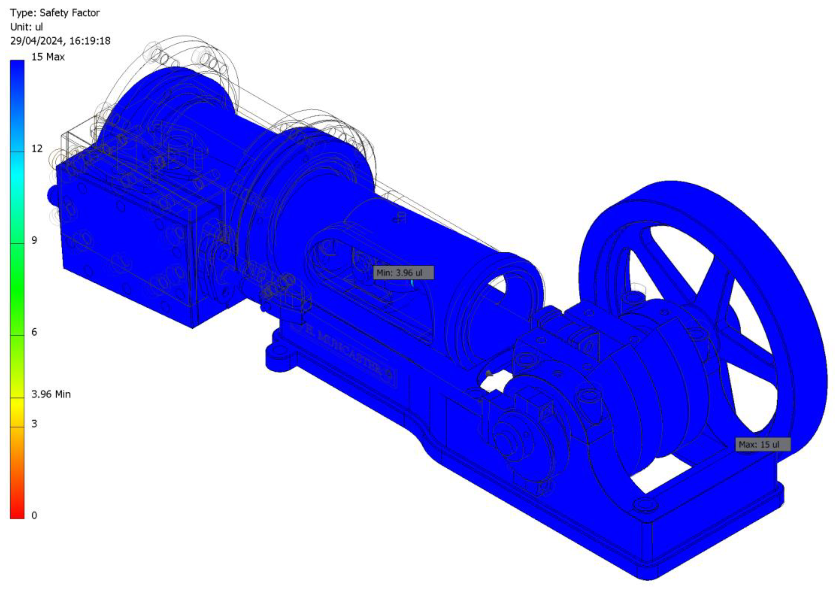
In addition, this working pressure value, which was obtained by observing the upper dead center as it is the most restrictive for this value, is the maximum so that, in both compression and traction, a safety factor is achieved of higher than 2. Moreover, it was verified which pressure value produces a safety factor of less than 4 (3.96), so the range of working pressures was obtained. On the other hand, the minimum pressure value was obtained by observing the lower dead center, which was the most restrictive at this value of 0.165 MPa (Figure 28).

Figure 28.
Safety factor distribution at a pressure of 0.165 MPa at the lower dead center position.
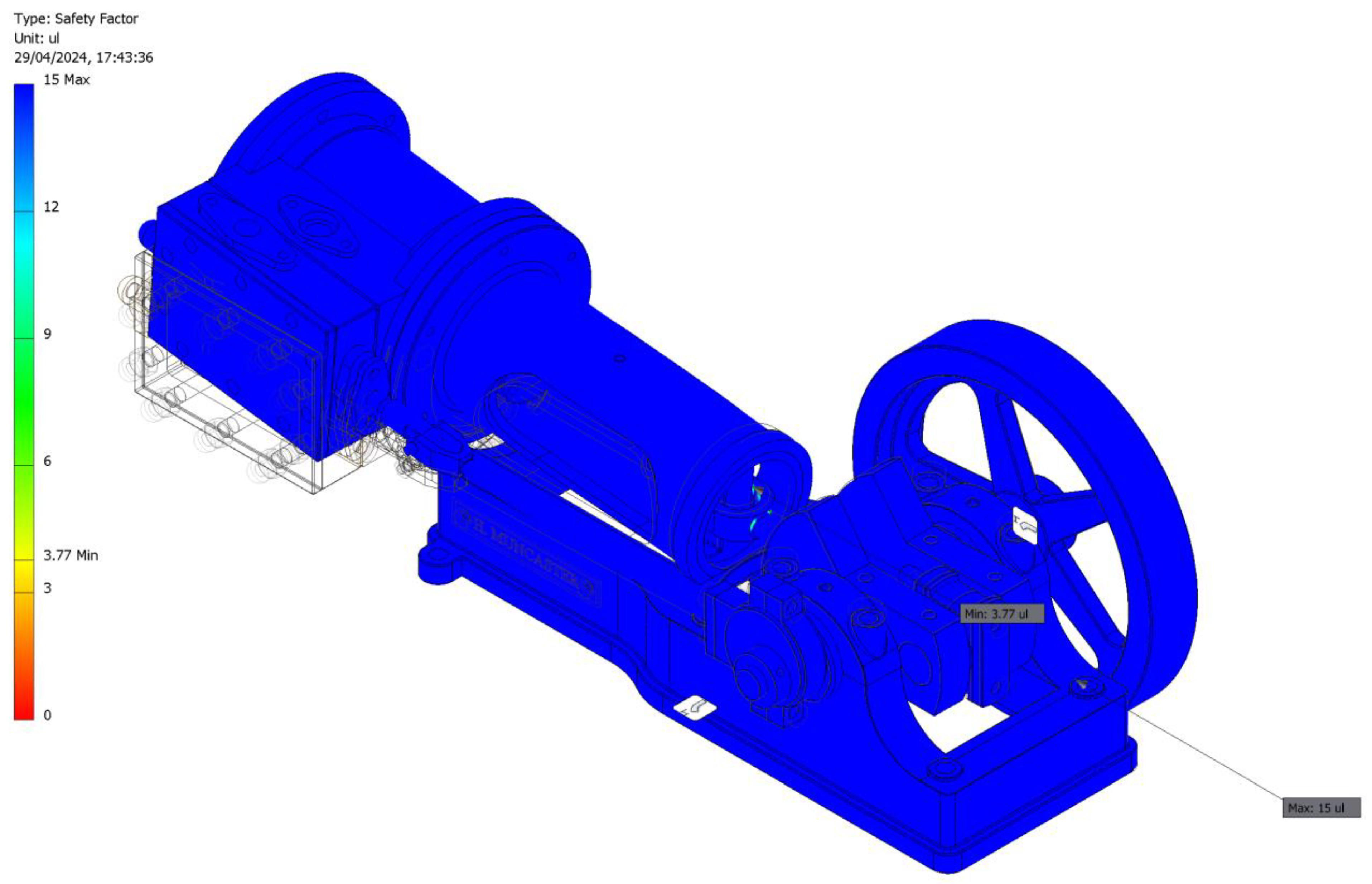
As a check, this pressure was also applied to the upper dead center, verifying that the safety factor is below 4 (3.77), as mentioned previously (Figure 29).

Figure 29.
Safety factor distribution at a pressure of 0.165 MPa at the upper dead center position.
Therefore, it can be stated that the operating range of steam intake pressure would be between 0.165 MPa and 0.320 MPa, so that the safety factor is always at a value of between 2 and 4.
4. Conclusions
In this study, the mechanical behavior of a single-cylinder horizontal steam engine equipped with a crosshead trunk guide was evaluated using FEM. A linear static analysis was conducted utilizing the stress analysis module integrated within the Autodesk Inventor Professional 2024 software, focusing on the engine’s behavior at two critical positions: lower dead center and upper dead center.
The primary objective of this research was to ascertain the maximum permissible working pressure to achieve optimal efficiency, alongside identifying the ideal range of working pressures for proper operation based on material strength criteria. This specifically involved considering an optimal safety factor range between 2 and 4.
Following manual mesh refinement, a mesh convergence analysis was conducted, resulting in a relative error of 4.74% in the third iteration for an element size of 2.50 mm at the lower dead center position and 2.55% in the second iteration for the same mean element size at the upper dead center position. The simulation outcomes indicated that the optimal working pressure range lies between 0.165 and 0.320 MPa.
At the maximum permissible pressure of 0.32 MPa, which yielded a minimum safety factor close to 2, the linear static analysis results were obtained. The von Mises stress values were found to peak at 54.36 MPa at the juncture of the piston rod and connecting rod (crosshead) in the lower dead center position and at 90.90 MPa on the connecting rod in the upper dead center position. The minimum safety factors were 2.35 at the lower dead center and 2.04 at the upper dead center, ensuring the design’s integrity and maintaining the safety factor within the optimal design range of 2 to 4.
Future research could involve performing a dimensional analysis after establishing the working pressure of 0.320 MPa to correlate the machine’s key dimensions (such as piston diameter, cylinder length, or flywheel diameter) and extrapolate the findings to other geometrically similar machines.
Author Contributions
Conceptualization, J.I.R.-S.; methodology, J.I.R.-S. and J.C.B.-M.; investigation, J.I.R.-S. and J.C.B.-M.; formal analysis, J.I.R.-S. and J.C.B.-M.; visualization, J.I.R.-S. and J.C.B.-M.; supervision, J.I.R.-S.; writing—original draft preparation, J.I.R.-S. and J.C.B.-M.; writing—review and editing, J.I.R.-S. and J.C.B.-M. All authors have read and agreed to the published version of the manuscript.
Funding
The research presented in this paper was possible thanks to a collaboration grant with the Department of Engineering Graphics, Design and Projects of the University of Jaen obtained in the 2023 call from the Ministry of Education and Vocational Training of the Government of Spain.
Institutional Review Board Statement
Not applicable.
Informed Consent Statement
Not applicable.
Data Availability Statement
The original contributions presented in the study are included in the article; further inquiries can be directed to the corresponding author.
Acknowledgments
We would like to thank the anonymous reviewers of this paper for their constructive suggestions and comments.
Conflicts of Interest
The authors declare no conflicts of interest.
References
- Inkster, I. (Ed.) History of Technology; Bloomsbury Academic: London, UK, 2004. [Google Scholar]
- Stokes, P.R. Piston steam engine innovation. Proc. Inst. Mech. Eng. Part A J. Power Energy 1996, 210, 95–98. [Google Scholar] [CrossRef]
- Rojas-Sola, J.I.; Galán-Moral, B.; De la Morena-de la Fuente, E. Agustín de Betancourt’s double-acting steam engine: Geometric modeling and virtual reconstruction. Symmetry 2018, 10, 351. [Google Scholar] [CrossRef]
- Rojas-Sola, J.I.; De la Morena-de la Fuente, E. Agustín de Betancourt’s double-acting steam engine: Analysis through computer-aided engineering. Appl. Sci. 2018, 8, 2309. [Google Scholar] [CrossRef]
- Wang, Y.; Zhou, Z.J.; Zhou, J.H.; Liu, J.Z.; Wang, Z.H.; Cen, K.F. Micro Newcomen steam engine using two-phase working fluid. Energy 2011, 36, 917–921. [Google Scholar] [CrossRef]
- Yatsuzuka, S.; Niiyama, Y.; Fukuda, K.; Muramatsu, K.; Shikazono, N. Experimental and numerical evaluation of liquid-piston steam engine. Energy 2015, 87, 1–9. [Google Scholar] [CrossRef]
- Thoendel, E. Simulation model of the thermodynamic cycle of a three-cylinder double-acting steam engine. Chem. Prod. Process Model. 2008, 3, 21. [Google Scholar] [CrossRef]
- Who Was Henry Muncaster? Available online: https://modelengineeringwebsite.com/Henry_Muncaster.html (accessed on 22 May 2024).
- Muncaster, H. Model Stationary Engines—Their Design and Construction; TEE Publishing Ltd.: Oxford, UK, 1912. [Google Scholar]
- Westbury, E.T. The Muncaster steam-engine models: A simple oscillating engine. Model Eng. 1957, 116, 270–272. [Google Scholar]
- Westbury, E.T. The Muncaster steam-engine models: Double-acting oscillating engines. Model Eng. 1957, 116, 337–339. [Google Scholar]
- Westbury, E.T. The Muncaster steam-engine models: Simple slide-valve engines. Model Eng. 1957, 116, 420–422. [Google Scholar]
- Westbury, E.T. The Muncaster steam-engine models: Horizontal stationary engines. Model Eng. 1957, 116, 488–490, 515. [Google Scholar]
- Westbury, E.T. The Muncaster steam-engine models: Vertical stationary engines. Model Eng. 1957, 116, 555–557. [Google Scholar]
- Westbury, E.T. The Muncaster steam-engine models: The simple and compound twin engines. Model Eng. 1957, 116, 634–636, 656. [Google Scholar]
- Westbury, E.T. The Muncaster steam-engine models: Entablature or table engines. Model Eng. 1957, 116, 700–702. [Google Scholar]
- Westbury, E.T. The Muncaster steam-engine models: Governors and control gear. Model Eng. 1957, 116, 778–780. [Google Scholar]
- Westbury, E.T. The Muncaster steam-engine models. Model Eng. 1957, 116, 841–843. [Google Scholar]
- Ceccarelli, M.; Cocconcelli, M. Plans for a Course on the History of Mechanisms and Machine Science. In Trends in Educational Activity in the Field of Mechanism and Machine Theory; Springer: Cham, Switzerland, 2022; pp. 135–144. [Google Scholar] [CrossRef]
- Cocconcelli, M.; Ceccarelli, M. Italian teaching with models from mechanism catalogues in 19th century. In Explorations in the History and Heritage of Machines and Mechanisms; Springer: Cham, Switzerland, 2024; pp. 18–30. [Google Scholar] [CrossRef]
- Ceccarelli, M.; Cocconcelli, M. Italian historical developments of teaching and museum valorization of mechanism models. Machines 2022, 10, 628. [Google Scholar] [CrossRef]
- Ceccarelli, M.; Koetsier, T. Burmester and Allievi: A theory and its application for mechanism design at the end of 19th century. J. Mech. Des. 2008, 130, 072301. [Google Scholar] [CrossRef]
- Fang, Y.; Ceccarelli, M. Peculiarities of evolution of machine technology and its industrialization in Italy during 19th century. Adv. Hist. Stud. 2015, 4, 338–355. [Google Scholar] [CrossRef]
- Fang, Y.; Ceccarelli, M. Findings on Italian historical developments of machine technology in 19th century towards industrial revolution. In The 11th IFToMM International Symposium on Science of Mechanisms and Machines; Springer: Cham, Switzerland, 2013; pp. 493–501. [Google Scholar] [CrossRef]
- Rojas-Sola, J.I.; Barranco-Molina, J.C. Analysis from functional viewpoint of a single-cylinder horizontal steam engine with a crosshead trunk guide through engineering graphics. Symmetry 2024, 16, 722. [Google Scholar] [CrossRef]
- Single-Cylinder Horizontal Steam Engine with a Crosshead Trunk Guide. Available online: https://modelengineeringwebsite.com/Muncaster_4c_mill_engine.html (accessed on 22 May 2024).
- Liu, Y.; Huang, M.; An, Q.; Bai, L.; Shang, D.Y. Dynamic characteristic analysis and structural optimization design of the large mining headrame. Machines 2022, 10, 510. [Google Scholar] [CrossRef]
- Stavroulakis, G.E.; Charalambidi, B.G.; Koutsianitis, P. Review of computational mechanics, optimization, and machine learning tools for digital twins applied to infrastructures. Appl. Sci. 2022, 12, 11997. [Google Scholar] [CrossRef]
- Rojas-Sola, J.I.; Gutiérrez-Antúnez, J.F. Analysis of the design of Henry Muncaster’s two-cylinder compound vertical steam engine with speed control. Appl. Sci. 2023, 13, 9150. [Google Scholar] [CrossRef]
- Shih, R.H.; Jumper, L. Parametric Modeling with Autodesk Inventor 2024; SDC Publications: Mission, KS, USA, 2023. [Google Scholar]
- Zienkiewicz, O.C.; Taylor, R.L. The Finite Element Method: Volume 1: The Basis, 5th ed.; Butterworth-Heinemann: Oxford, UK, 2000. [Google Scholar]
- Reddy, J.N. An Introduction to the Finite Element Method, 3rd ed.; McGraw-Hill: New York, NY, USA, 2006. [Google Scholar]
- Gere, J.M.; Goodno, B.J. Mechanics of Materials, 8th ed.; Cengage Learning: Stamford, CT, USA, 2012. [Google Scholar]
- Timoshenko, S.; Goodier, J.N. Theory of Elasticity, 2nd ed.; McGraw-Hill: New York, NY, USA, 1951. [Google Scholar]
- Branch Education in Spanish: ¿Cómo Funcionan los Motores de Vapor? Available online: https://www.youtube.com/watch?v=Cmys_-um0C4&t=489s (accessed on 13 May 2024).


Disclaimer/Publisher’s Note: The statements, opinions and data contained in all publications are solely those of the individual author(s) and contributor(s) and not of MDPI and/or the editor(s). MDPI and/or the editor(s) disclaim responsibility for any injury to people or property resulting from any ideas, methods, instructions or products referred to in the content. |
© 2024 by the authors. Licensee MDPI, Basel, Switzerland. This article is an open access article distributed under the terms and conditions of the Creative Commons Attribution (CC BY) license (https://creativecommons.org/licenses/by/4.0/).