
Transient Dynamic Response of Generally Shaped Arches under Interval Uncertainties


Abstract
1. Introduction
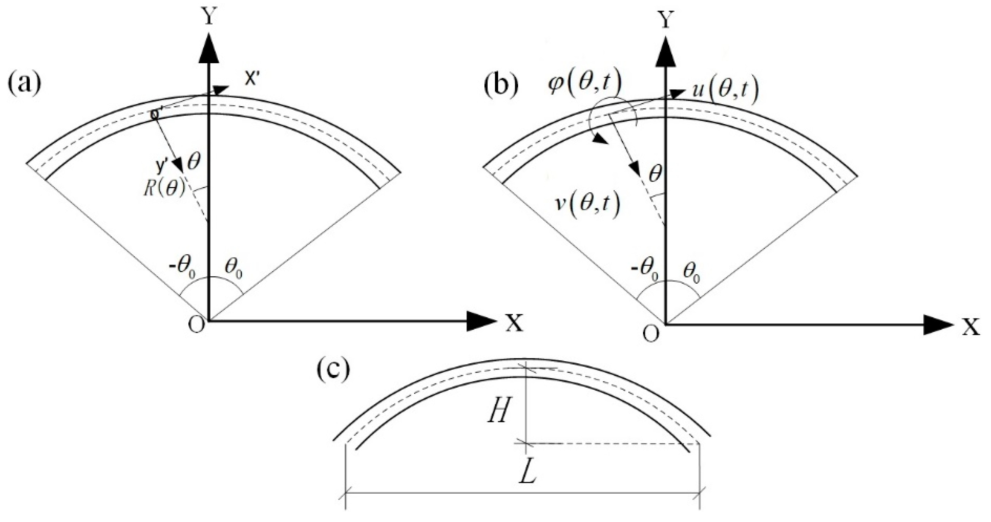
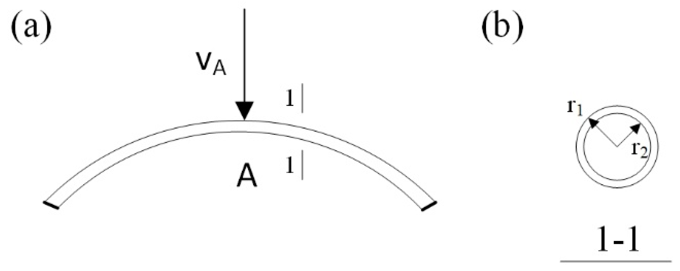
2. Generally Shaped Arch Model and Equations of Motion
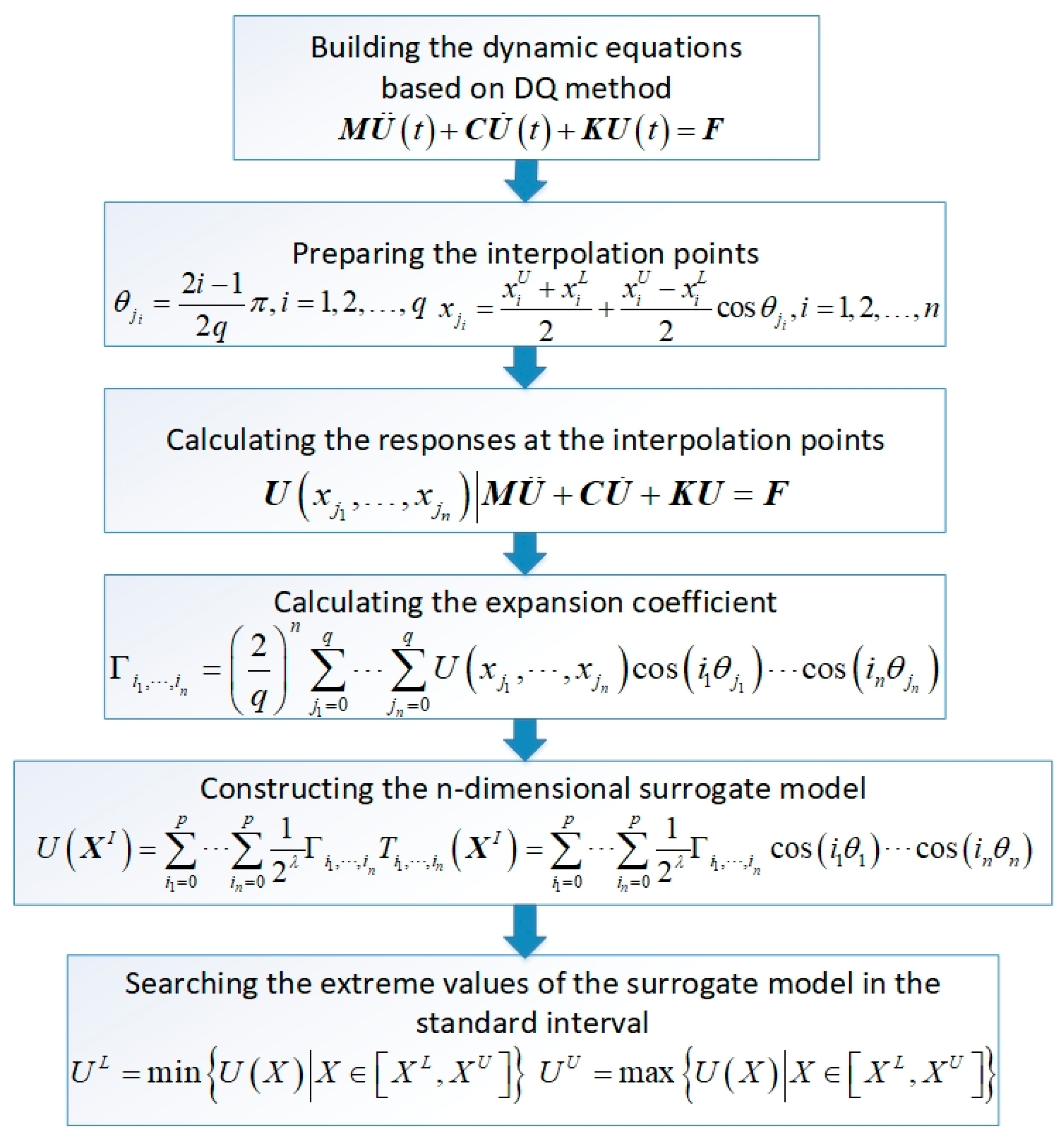
3. Chebyshev Polynomial Approximation Method for Dynamic Responses
4. Numerical Results and Discussion
4.1. Comparison of the Chebyshev Interval Method with the Scanning Method in Transient Responses Calculation
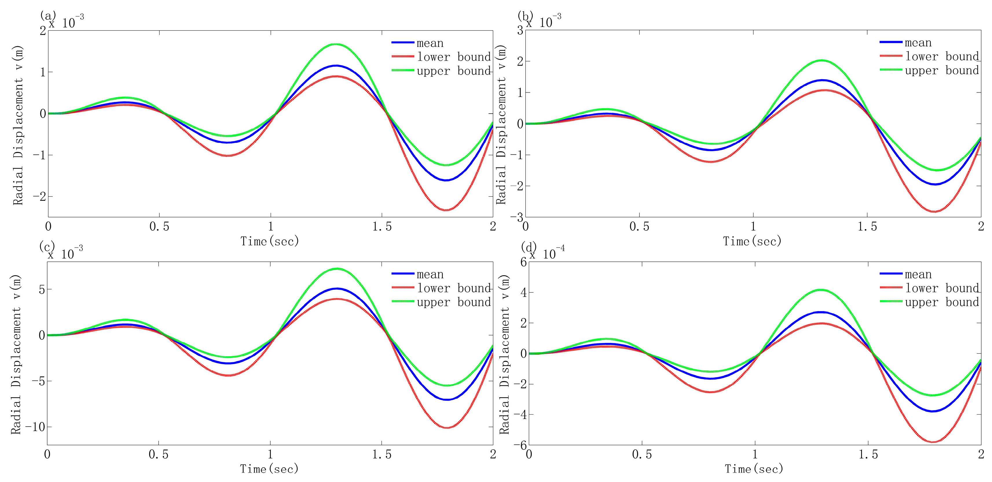
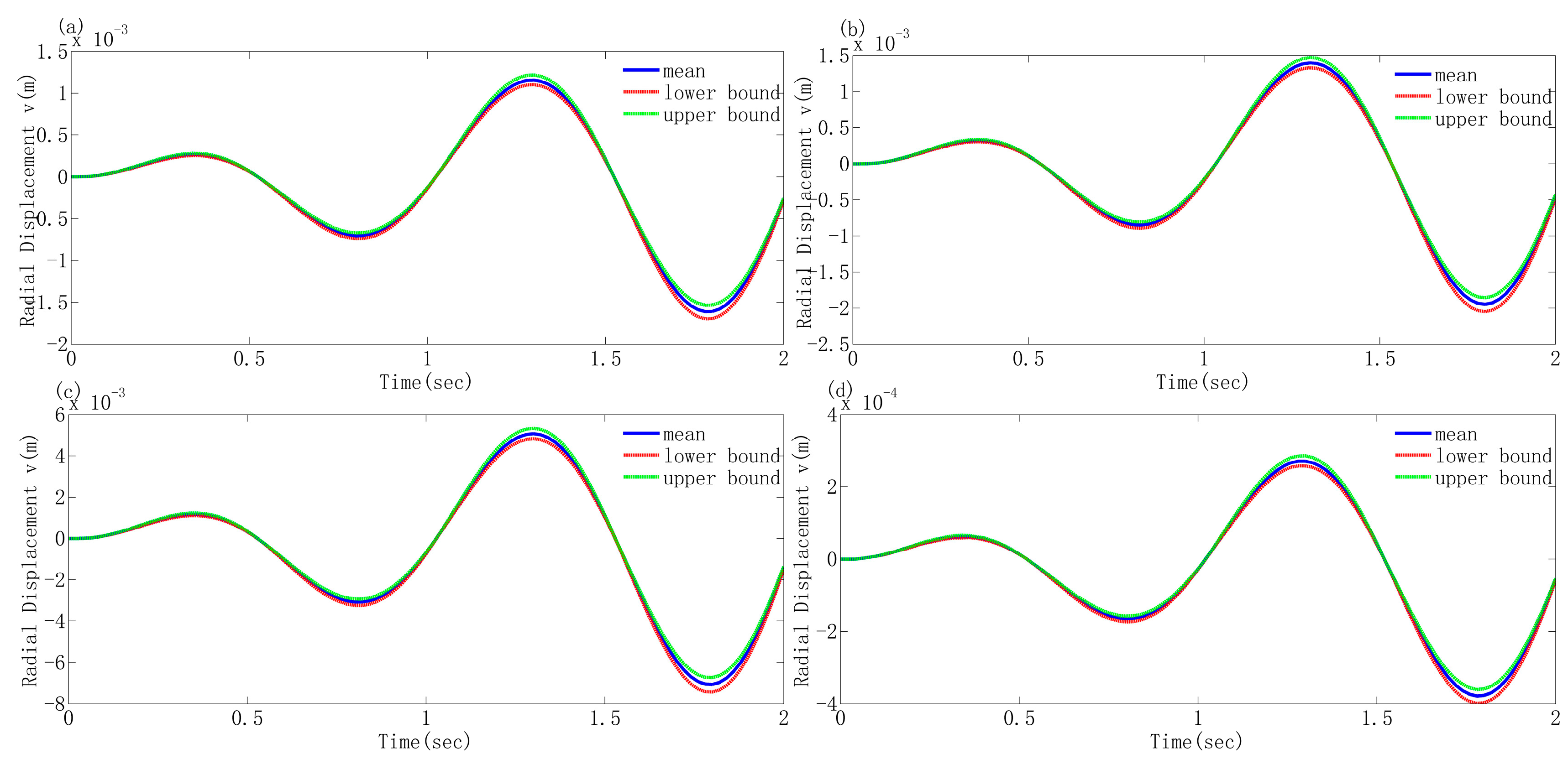
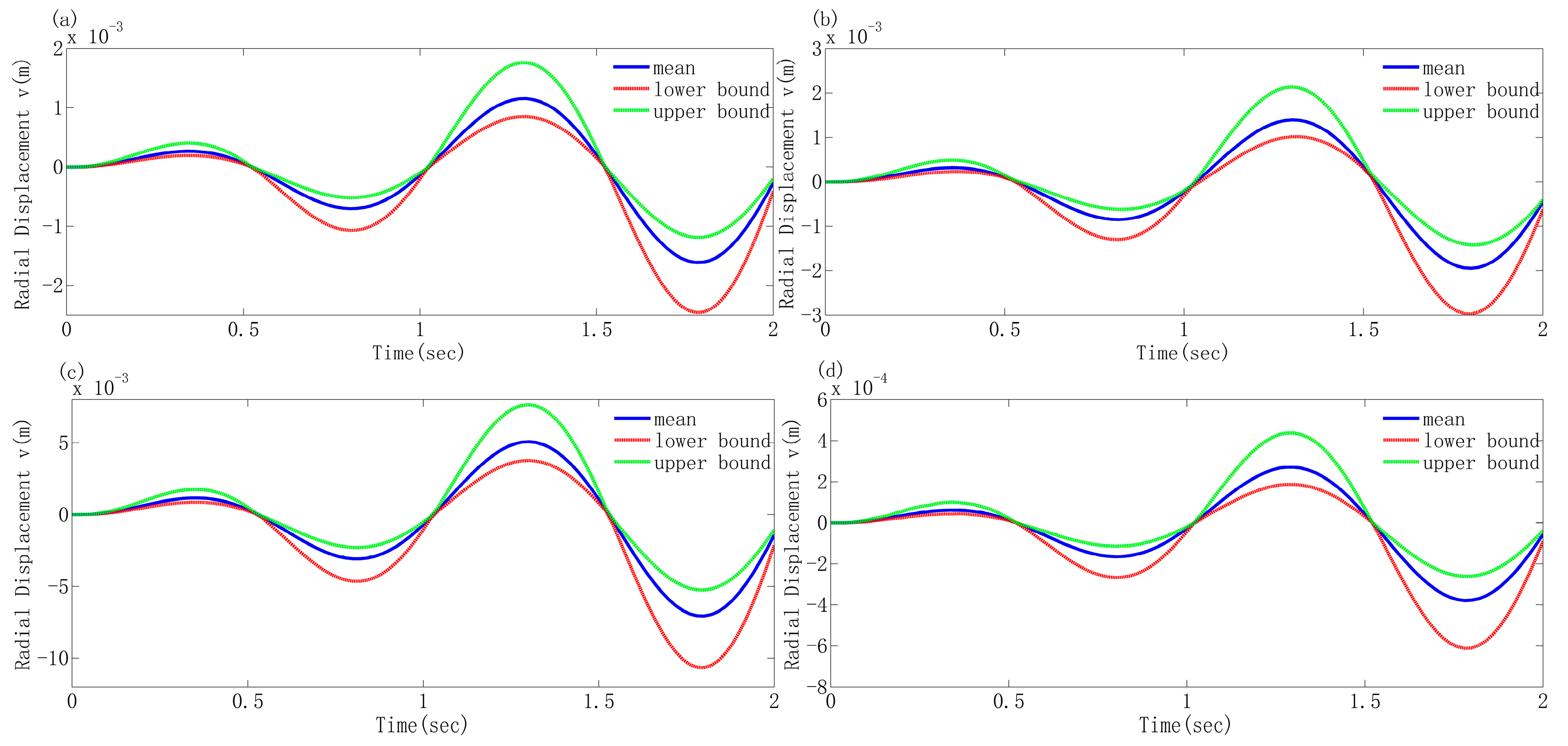
4.2. Transient Dynamic Behavior Investigation of the Generally Shaped Arches Considering Different Uncertain Parameters
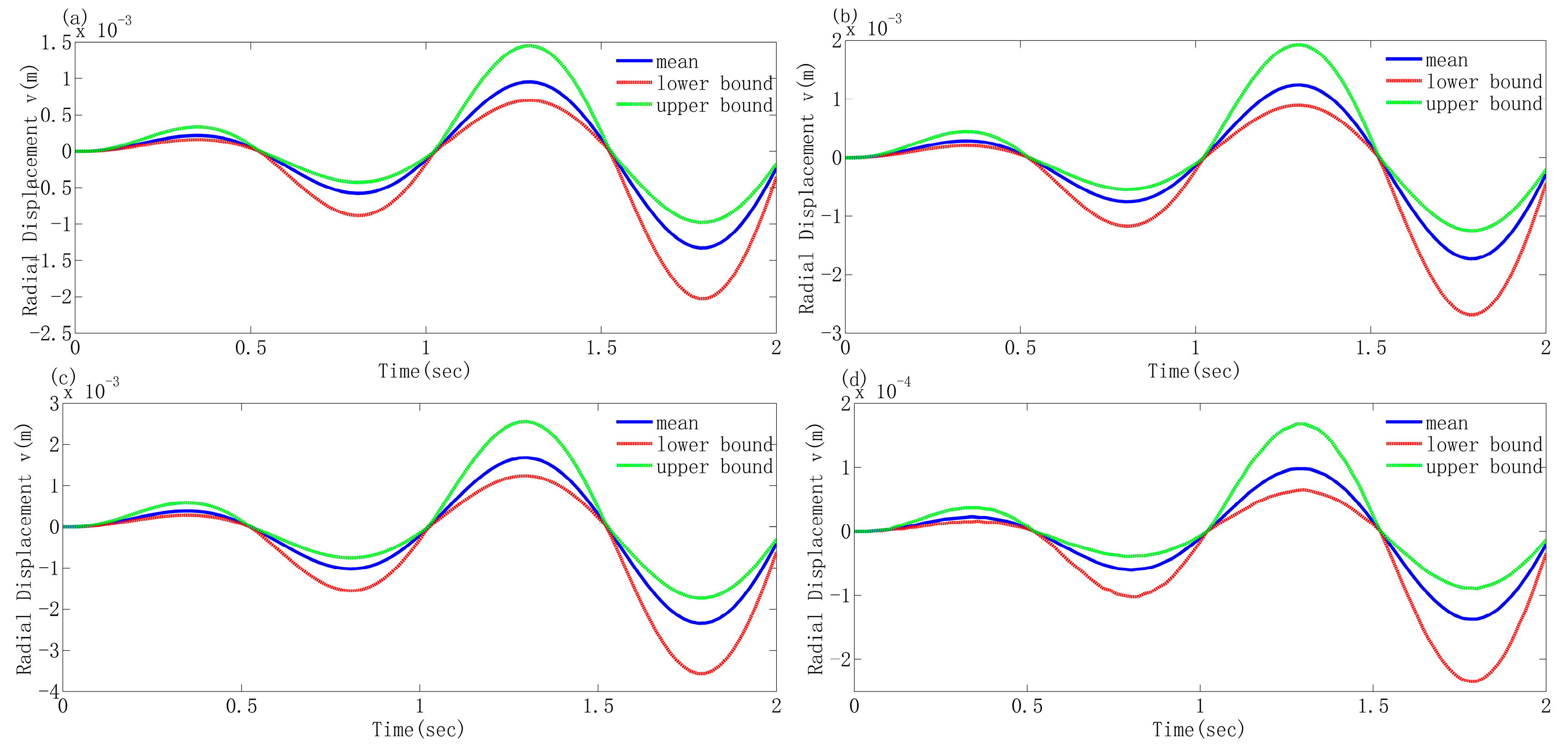
4.3. Transient Dynamic Responses Comparison of General Shaped Arches with the Same Total Length and Different Mid-Span Height
5. Conclusions
- Different uncertain parameters exert varying influences on the responses. The cross-sectional geometric parameters (the inner radius of the circular tube cross-section) have a more significant influence on the uncertain responses than Young’s modulus. Moreover, the greater the absolute value of the deterministic response, the more pronounced this influence becomes. When considering these two uncertain parameters concurrently, the influence of the cross-sectional geometric parameter is predominant.
- Arches of different shapes with the same rise span ratio exhibit distinct deterministic responses and corresponding uncertain responses under the same external excitation. Through comparison, it is observed that the response of the elliptical arch is the greatest and that of the parabolic arch is the smallest. When the rise span ratio is increased while maintaining the span constant, the responses of each arch decrease, and the above conclusion still holds, indicating that the shape and rise span ratio of the arch are the primary factors influencing the dynamic response.
Author Contributions
Funding
Institutional Review Board Statement
Informed Consent Statement
Data Availability Statement
Conflicts of Interest
References
- Caliò, I.; D’Urso, D.; Greco, A. The Influence of Damage on the Eigen-Properties of Timoshenko Spatial Arches. Comput. Struct. 2017, 190, 13–24. [Google Scholar] [CrossRef]
- Caliò, I.; Greco, A.; D’Urso, D. Free Vibrations of Spatial Timoshenko Arches. J. Sound Vib. 2014, 333, 4543–4561. [Google Scholar] [CrossRef]
- Eftekhari, S.A. Differential Quadrature Procedure for in-Plane Vibration Analysis of Variable Thickness Circular Arches Traversed by a Moving Point Load. Appl. Math. Model. 2016, 40, 4640–4663. [Google Scholar] [CrossRef]
- Eroglu, U.; Ekrem, T. Crack Modeling and Identification in Curved Beams Using Differential Evolution. Int. J. Mech. Sci. 2017, 131–132, 435–450. [Google Scholar] [CrossRef]
- Tornabene, F.; Dimitri, R.; Viola, E. Transient Dynamic Response of Generally-Shaped Arches Based on a Gdq-Time-Stepping Method. Int. J. Mech. Sci. 2016, 114, 277–314. [Google Scholar] [CrossRef]
- Zhong, Z.; Liu, A.; Fu, J.; Pi, Y.-L.; Deng, J.; Xie, Z. Analytical and Experimental Studies on out-of-Plane Dynamic Parametric Instability of a Circular Arch under a Vertical Harmonic Base Excitation. J. Sound Vib. 2021, 500, 116011. [Google Scholar] [CrossRef]
- Zhong, Z.; Liu, A.; Pi, Y.-L.; Deng, J.; Fu, J.; Gao, W. In-Plane Dynamic Instability of a Shallow Circular Arch under a Vertical-Periodic Uniformly Distributed Load Along the Arch Axis. Int. J. Mech. Sci. 2021, 189, 105973. [Google Scholar] [CrossRef]
- Gusella, V. Geometrical Uncertainty in Mechanics and Random Curves in Space. Probab. Eng. Mech. 2020, 62, 103102. [Google Scholar] [CrossRef]
- Wu, B.; Wu, D.; Gao, W.; Song, C. Time-Variant Random Interval Response of Concrete-Filled Steel Tubular Composite Curved Structures. Compos. Part B Eng. 2016, 94, 122–138. [Google Scholar] [CrossRef]
- Wu, B.; Gao, W.; Wu, D.; Song, C. Probabilistic Interval Geometrically Nonlinear Analysis for Structures. Struct. Saf. 2017, 65, 100–112. [Google Scholar] [CrossRef]
- Hacıefendioğlu, K.; Başağa, H.B.; Banerjee, S. Probabilistic Analysis of Historic Masonry Bridges to Random Ground Motion by Monte Carlo Simulation Using Response Surface Method. Constr. Build. Mater. 2017, 134, 199–209. [Google Scholar] [CrossRef]
- Hong, G.; Deng, Z. Dynamic Response Analysis of Nonlinear Structures with Hybrid Uncertainties. Appl. Math. Model. 2023, 119, 174–195. [Google Scholar] [CrossRef]
- Tsoulos, I.G.; Stavrou, V.; Mastorakis, N.E.; Tsalikakis, D. Genconstraint: A Programming Tool for Constraint Optimization Problems. SoftwareX 2019, 10, 100355. [Google Scholar] [CrossRef]
- Meng, D.; Hu, Z.; Guo, J.; Lv, Z.; Xie, T.; Wang, Z. An Uncertainty-Based Structural Design and Optimization Method with Interval Taylor Expansion. Structures 2021, 33, 4492–4500. [Google Scholar] [CrossRef]
- Qiu, Z.; Zhang, Z. Crack Propagation in Structures with Uncertain-but-Bounded Parameters Via Interval Perturbation Method. Theor. Appl. Fract. Mech. 2018, 98, 95–103. [Google Scholar] [CrossRef]
- Wu, J.; Luo, Z.; Zhang, N.; Zhang, Y. A New Interval Uncertain Optimization Method for Structures Using Chebyshev Surrogate Models. Comput. Struct. 2015, 146, 185–196. [Google Scholar] [CrossRef]
- Wu, J.; Zhang, Y.; Chen, L.; Luo, Z. A Chebyshev Interval Method for Nonlinear Dynamic Systems under Uncertainty. Appl. Math. Model. 2013, 37, 4578–4591. [Google Scholar] [CrossRef]
- Wei, T.; Li, F.; Meng, G.; Li, H. A Univariate Chebyshev Polynomials Method for Structural Systems with Interval Uncertainty. Probab. Eng. Mech. 2021, 66, 103172. [Google Scholar] [CrossRef]
- Yan, D.; Zheng, Y.; Liu, W.; Chen, T.; Chen, Q. Interval Uncertainty Analysis of Vibration Response of Hydroelectric Generating Unit Based on Chebyshev Polynomial. Chaos Solitons Fractals 2022, 155, 111712. [Google Scholar] [CrossRef]
- Jia, Z.; Yang, Y.; Zheng, Q.; Deng, W. Dynamic Analysis of Jeffcott Rotor under Uncertainty Based on Chebyshev Convex Method. Mech. Syst. Signal Process. 2022, 167, 108603. [Google Scholar] [CrossRef]
- Fu, C.; Sinou, J.-J.; Zhu, W.; Lu, K.; Yang, Y. A State-of-the-Art Review on Uncertainty Analysis of Rotor Systems. Mech. Syst. Signal Process. 2023, 183, 109619. [Google Scholar] [CrossRef]
- Fu, C.; Zhu, W.; Zheng, Z.; Sun, C.; Yang, Y.; Lu, K. Nonlinear Responses of a Dual-Rotor System with Rub-Impact Fault Subject to Interval Uncertain Parameters. Mech. Syst. Signal Process. 2022, 170, 108827. [Google Scholar] [CrossRef]
- Li, F.; Li, H.; Zhao, H.; Zhou, Y. A Dimension-Reduction Based Chebyshev Polynomial Method for Uncertainty Analysis in Composite Corrugated Sandwich Structures. J. Compos. Mater. 2022, 56, 1891–1900. [Google Scholar] [CrossRef]
- Mercier, A.; Jézéquel, L. Nonlinear and Stochastic Analysis of Dynamical Instabilities Based on Chebyshev Polynomial Properties and Applied to a Mechanical System with Friction. Mech. Syst. Signal Process. 2023, 189, 110051. [Google Scholar] [CrossRef]
- Mo, J.; Yan, W.-J.; Yuen, K.V.; Beer, M. Efficient Inner-Outer Decoupling Scheme for Non-Probabilistic Model Updating with High Dimensional Model Representation and Chebyshev Approximation. Mech. Syst. Signal Process. 2023, 188, 110040. [Google Scholar] [CrossRef]
- Xiang, W.; Yan, S.; Wu, J.; Niu, W. Dynamic Response and Sensitivity Analysis for Mechanical Systems with Clearance Joints and Parameter Uncertainties Using Chebyshev Polynomials Method. Mech. Syst. Signal Process. 2020, 138, 106596. [Google Scholar] [CrossRef]
- Zhao, H.; Fu, C.; Zhang, Y.; Zhu, W.; Lu, K.; Francis, E.M. Dimensional Decomposition-Aided Metamodels for Uncertainty Quantification and Optimization in Engineering: A Review. Comput. Methods Appl. Mech. Eng. 2024, 428, 117098. [Google Scholar] [CrossRef]
- Zhao, S.; Ren, X.; Zheng, Q.; Lu, K.; Fu, C.; Yang, Y. Transient Dynamic Balancing of the Rotor System with Uncertainty. Mech. Syst. Signal Process. 2022, 171, 108894. [Google Scholar] [CrossRef]


| Type of Arch | Geometry Description | Parametric Representation | Curvature Radius Concerning θ |
|---|---|---|---|
| Circumference | 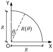 | R(θ) = R | |
| Cycloid | 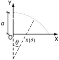 | R(θ) = 4acosθ | |
| Ellipse | 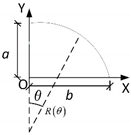 | ||
| Parabola | 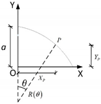 |
| Description | Value |
|---|---|
| Young’s modulus E | 210 Gpa |
| Density of mass ρ | 7860 kg/m3 |
| Poisson ratio υ | 0.3 |
| Outer radius r1 | 0.09 m |
| Inner radius r2 | 0.078 m |
| Shear factor κ | 1.2 |
| Type | Description | Value | |
|---|---|---|---|
| Case 1 | Linear increasing concentrated load | 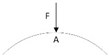 | F1 = 20t (kN) |
| Case 2 | Harmonic concentrated load |  | F2 = 20 × sin(2πt) (kN) |
| Case 3 | Harmonic distributed load with a linear increasing variation |  | F3 = 20t × sin(2πt) (kN/m) |
| Case 4 | Harmonic distributed load with negative exponential variation |  | F4 = 20 × e−t/2 × sin(2πt) (kN/m) |
| Size | Response Type | Circumference | Cycloid | Ellipse | Parabola | ||
|---|---|---|---|---|---|---|---|
| H = 3 m L = 10 m | Deterministic | 1.156 | 1.396 | 5.073 | 0.271 | ||
| IRCS * | Lower | 0.893 | 1.069 | 3.959 | 0.197 | ||
| Upper | 1.673 | 2.027 | 7.267 | 0.416 | |||
| YM * | Lower | 1.101 | 1.330 | 4.831 | 0.258 | ||
| Upper | 1.217 | 1.470 | 5.340 | 0.286 | |||
| Both * | Lower | 0.851 | 1.018 | 3.770 | 0.187 | ||
| Upper | 1.761 | 2.133 | 7.650 | 0.438 | |||
| H = 4 m L = 10 m | Deterministic | 0.953 | 1.240 | 1.681 | 0.098 | ||
| Both * | Lower | 0.701 | 0.895 | 1.240 | 0.064 | ||
| Upper | 1.452 | 1.926 | 2.557 | 0.168 | |||
| Size | Response Type | Circumference | Cycloid | Ellipse | Parabola | ||
|---|---|---|---|---|---|---|---|
| H = 3 m L = 10 m | Deterministic | −1.611 | −1.948 | −7.068 | −0.379 | ||
| IRCS * | Lower | −2.333 | −2.825 | −10.125 | −0.581 | ||
| Upper | −1.245 | −1.491 | −5.516 | −0.275 | |||
| YM * | Lower | −1.696 | −2.050 | −7.440 | −0.399 | ||
| Upper | −1.535 | −1.855 | −6.731 | −0.361 | |||
| Both * | Lower | −2.455 | −2.974 | −10.658 | −0.612 | ||
| Upper | −1.186 | −1.421 | −5.253 | −0.261 | |||
| H = 4 m L = 10 m | Deterministic | −1.328 | −1.730 | −2.343 | −0.137 | ||
| Both * | Lower | −2.023 | −2.686 | −3.562 | −0.234 | ||
| Upper | −0.977 | −1.248 | −1.728 | −0.089 | |||
Disclaimer/Publisher’s Note: The statements, opinions and data contained in all publications are solely those of the individual author(s) and contributor(s) and not of MDPI and/or the editor(s). MDPI and/or the editor(s) disclaim responsibility for any injury to people or property resulting from any ideas, methods, instructions or products referred to in the content. |
© 2024 by the authors. Licensee MDPI, Basel, Switzerland. This article is an open access article distributed under the terms and conditions of the Creative Commons Attribution (CC BY) license (https://creativecommons.org/licenses/by/4.0/).
Share and Cite
Nie, Z.; Fu, C.; Yang, Y.; Zhao, J. Transient Dynamic Response of Generally Shaped Arches under Interval Uncertainties. Appl. Sci. 2024, 14, 5918. https://doi.org/10.3390/app14135918
Nie Z, Fu C, Yang Y, Zhao J. Transient Dynamic Response of Generally Shaped Arches under Interval Uncertainties. Applied Sciences. 2024; 14(13):5918. https://doi.org/10.3390/app14135918
Chicago/Turabian StyleNie, Zhihua, Chao Fu, Yongfeng Yang, and Jiepeng Zhao. 2024. "Transient Dynamic Response of Generally Shaped Arches under Interval Uncertainties" Applied Sciences 14, no. 13: 5918. https://doi.org/10.3390/app14135918
APA StyleNie, Z., Fu, C., Yang, Y., & Zhao, J. (2024). Transient Dynamic Response of Generally Shaped Arches under Interval Uncertainties. Applied Sciences, 14(13), 5918. https://doi.org/10.3390/app14135918