Abstract
The paper proposes an innovative adaptation of the estimation of distribution algorithm (EDA), intended for multi-objective optimisation of a ship’s route in a non-stationary environment (tidal waters). The key elements of the proposed approach—the adaptive Markov chain-based path generator and the dynamic programming-based local search algorithm—are presented in detail. The experimental results presented indicate the high effectiveness of the proposed algorithm in finding very good quality approximations of optimal solutions in the Pareto sense. Critical for this was the proposed local search algorithm, whose application improved the final result significantly (the Pareto set size increased from five up to nine times, and the Pareto front quality just about doubled). The proposed algorithm can also be applied to other domains (e.g., mobile robot path planning). It can be considered a framework for (simulation-based) multi-objective optimal path planning in non-stationary environments.
1. Introduction
The importance of maritime cargo transport is on the rise. It is estimated that approximately 80% of goods are transported by sea, and this amount is constantly increasing. At the same time, there is a greater need to reduce carbon emissions—in 2018, the International Maritime Organization set the goal of reducing emissions by 40% (compared to 2008) per transport unit by 2030 [1]. As a result, fuel consumption reduction and optimal navigation have become more important than ever [2,3,4,5].
A significant number of real-life maritime transport optimisation problems are very complex [6], mainly because they are at the same time multi-objective (the route should be optimal at least in terms of passage time and fuel consumption), non-stationary (due to tidal streams and changing weather conditions), and variational (the search space consists of trajectories). The only solution methods that can be effective for such cases are simulation based, which naturally leads to the use of meta-heuristic algorithms [7].
Meta-heuristics typically require special mechanisms to maintain the population diversity to avoid getting stuck in local optima—this stops the search process and is particularly unfavourable when looking for the Pareto front. Unfortunately, diversity control mechanisms can result in a loss of exploitability, and this is why we often use local search algorithms simultaneously. The local search component becomes particularly important in the context of variational problems since, in most cases, the probability of missing a non-dominated solution (i.e., an element of the Pareto set) is significantly higher than in non-variational optimisation problems. This stems mainly from an assumed (non-obvious) distance representation in the search space and the corresponding implementation of a local perturbation, which should mimic trajectory variation.
Considering all the above-mentioned properties, to the best of our knowledge, there are no methods that effectively meet all these requirements, especially as far as the real-life applications are considered (a detailed review of the related research can be found in Section 2). Therefore, in this paper, we address this issue.
The main contributions of this paper are as follows:
- A 3D-graph-based design space and the computational topology it generates for dynamic programming (DP)-based local search (Section 4.1);
- An (inspired by the estimation of distribution algorithm) adaptive Markov chain-based path generator directing the global search process (Section 4.2);
- The dp-based local search algorithm, significantly boosting—thanks to its exploitation capabilities—the global search process (Section 4.3);
- The meta-heuristic algorithm combining the above elements to create an effective framework for (simulation based) multi-objective optimal path planning in non-stationary environments (Section 4.4);
- Experimental results showing the high effectiveness of the proposed algorithm in finding very good quality and diversified approximations of the set of Pareto optimal solutions (Section 5).
The remainder of this paper is organised as follows. Section 2 presents related research. Following that, in Section 3, the optimisation problem under consideration is defined, and the proposed algorithm is described in Section 4. Thereafter, experimental results are presented and discussed in Section 5. Finally, Section 6 contains the conclusion of the study.
2. Related Research
This section will discuss research work related to methods for the optimal ship routing in changing environmental conditions and estimation of distribution algorithms (EDAs). The differences between the proposed approach and methods known from the literature are also discussed.
2.1. Methods for Ship Routing Problem
Ship safety and energy efficiency are important factors for making ship operations more competitive and sustainable [4,8]. Therefore, more and more researchers are studying how to optimize ship routes based on weather and sea conditions [2,3,4,9,10]. These factors affect how fast a ship moves, how much fuel it uses, and how much energy it emits.
To find a solution, a ship routing problem is reduced to a two-dimensional subpath search problem, which considers only position and assumes that either the ship’s speed or main engine output stays the same [4,11]. The reduced ship weather routing problem is usually solved by using the modified isochrone method [12], the isopone method for the minimum-time problem [13], dynamic programming for ship route optimisation with minimising fuel oil consumption [14], and Dijkstra’s algorithm using the weather forecast data [15]. Metaheuristic approaches (for example, evolutionary algorithms) were also used to find the optimal ship route taking into account weather conditions [16] or the route length and fuel prices in visited ports [5]. Notwithstanding, in reality, the lengthy routes and significant fluctuations in weather and sea conditions render it impracticable to maintain a consistent sailing velocity and primary engine output for vessels traversing the ocean [4].
A number of three-dimensional optimisation algorithms have been proposed to better simulate fuel consumption. The sum of weighted criteria of fuel consumption and ship safety was used in a real-coded genetic algorithm for weather routing proposed in [17]. In another approach, time was taken into account as a third additional dimension in addition to two-dimensional space, and the three-dimensional problem formulated in this way was solved by adapting the three-dimensional isochrones method with weighting factors [18].
The more realistic model of fuel consumption, taking into account the effect of hull and propeller fouling, and ocean currents was proposed in [19]. In this work, a genetic algorithm was used to find the optimal ship’s path, and the goal was to minimize the fuel consumption.
The application of machine learning-based approaches included the use of models trained on real-world navigation data of ships in various weather conditions. The trained machine learning models were then used to predict fuel consumption and, consequently, optimise the ship’s route [20,21]. The Attention-Bidirectional Long Short-Term Memory model optimised by the Whale Optimisation Algorithm was used for ship trajectory prediction aimed at collision avoidance and safety increase [22]. Statistical models taking into account wave height, wave period, wind speed, and the engine’s RPM data were also used for ship route planning [23]. The goals of path optimisation in the case of such methods included safety, fuel consumption reduction, and on time arrival at the destination.
The ship weather routing problem was also solved using multi-objective optimisation algorithms. In [24], the two-objective ship routing problem was formulated as a non-linear integer programming problem. The objectives included minimising the fuel consumption and the total risk. Multi-objective evolutionary algorithms were used to solve the ship weather routing problem in [16,25,26,27,28]. In these works, various objectives were used, like estimated time of arrival, fuel consumption and safety. User preferences were taken into account in the multi-objective evolutionary algorithm with weight intervals proposed in [3]. In the presented approach, the ship’s route consisted of nodes including information about the location, estimated time of arrival, engine settings, and ship heading.
There were also attempts to solve the ship weather routing problem using three-dimensional dynamic programming algorithms. Minimising the ship fuel consumption was a goal of a 3D dynamic programming-based method proposed in [2]. In contrast to most of the research works on ship weather routing optimisation, the proposed approach modified both the engine power and heading settings during searching for an optimal path [2]. A similar approach, based on modifying both the ship heading and speed, was introduced in [4]. The proposed method was based on an improved 3D dynamic programming algorithm for ship route optimisation.
The approach proposed in this paper is distinguished by the use of an innovative adaptation of the estimation of distribution algorithm (EDA) for the multi-objective optimisation of a ship’s route in a non-stationary environment (tidal waters). The key elements of the proposed approach are the adaptive Markov chain-based path generator and the dynamic programming-based local search algorithm. The proposed approach is characterised by a unique set of features, both in terms of the problem instance being solved (ship routing in a non-stationary environment) and the methods used (multi-objective estimation of distribution algorithm, adaptive Markov chain-based path generator, and the use of the dynamic programming-based local search algorithm), which significantly distinguishes it from the methods discussed above (see Table 1).
2.2. Estimation of Distribution Algorithms
Estimation of distribution algorithms (EDAs) are a specific branch of evolutionary algorithms (EAs) characterised by a way of generating new solutions using a probability distribution model [29,30]. This model is estimated based on the best individuals currently available in the population. The random sampling of offspring individuals ensures population diversity and robustness of the algorithm [30,31].
Most of the proposed EDAs generate a set of new solutions using the estimated Gaussian model, and thus they are called Gaussian estimation of distribution algorithms (GEDAs) [30,32]. Two types of GEDAs can be distinguished based on whether the correlation between variables is taken into account, univariate GEDAs (UGEDAs) and multivariate GEDAs (MGEDAs), which obtain better results for problems with many interacting variables [31,32,33].
However, MGEDAs have problems with premature convergence in the case of multi-modal optimisation problems with many flat and wide basins of attraction due to the rapid reduction in variances [31,33]. To deal with this problem, many techniques for avoiding premature convergence and improving EDAs efficacy in the case of multi-modal optimisation problems have been proposed. Such techniques include a correlation-triggered adaptive covariance scaling strategy [34], a standard-deviation ratio indicator [35], a cross-entropy-based adaptive covariance scaling method [36], a multiple submodels maintenance technique [37], a multi-modal estimation of distribution algorithm based on cooperative clustering strategy [38], and a layered learning EDA, which maintains multiple probability distribution models in each generation [30].
Estimation of distribution algorithms have also been adapted for multi-objective optimisation problems. Multi-objective EDAs (MOEDAs) include, among others, the Multi-Objective Hierarchical Bayesian Optimisation Algorithm [39], Multi-Objective Mixed Bayesian Optimisation Algorithm [40], and Multi-Objective Extended Compact Genetic Algorithm [41]. Many-objective optimisation problems have been addressed by the Multi-Dimensional Bayesian Network Estimation of Distribution Algorithm [42]. EDA based on domain adaptation and non-parametric estimation for solving dynamic multi-objective optimisation problems was proposed in [43]. The Directed Multi-Objective Estimation of Distribution Algorithm proposed in [44] addressed the problem of premature stagnation of MOEDAs on local Pareto fronts. The proposed algorithm avoided stagnation by reorienting the covariance matrix of a multivariate Gaussian distribution.
Combinatorial optimisation is another area of research in which estimation of distribution algorithms have been used. An EDA-based algorithm for Unmanned Aerial Vehicle (UAV) path planning was proposed in [45]. A method using EDA for trajectory optimisation in low-thrust orbit transfers was introduced in [46].
Some EDAs for combinatorial optimisation problems were used together with local search algorithms. For example, a hybrid algorithm for the quadratic assignment problem, combining EDA and the 2-opt local search algorithm, was proposed in [47]. The authors of [48] used a hybrid of EDA and variable neighbourhood search (VNS) for minimising the total flowtime in the permutation flowshop scheduling problem. A hybrid of EDA and VNS was also applied to distributed flexible job shop scheduling with the crane transportation problem [49].
In this paper, an innovative adaptation of the estimation of distribution algorithm (EDA) for multi-objective optimisation of a ship’s route in a non-stationary environment (tidal waters) is proposed. The proposed method uses the adaptive Markov chain-based path generator and the dynamic programming-based local search algorithm. All these elements distinguish the proposed approach from the EDA algorithms discussed above (see Table 1).

Table 1.
Comparison of features of individual methods.
Table 1.
Comparison of features of individual methods.
| Method | Problem Features | Algorithm Features | |||||
|---|---|---|---|---|---|---|---|
| Combinatorial Optimisation | Multi-Objective Problem | Non-Stationary Problem | (Explicit) Probability Distribution Based | Local Search | Deterministic Local Search (with Tabu List) | ||
| Our method | YES | YES | YES | YES | YES | YES | |
| [2,4,12,13,14,15,19,20,21,22] | YES | NO | NO | NO | NO | NO | |
| [3,5,16,17,18,23,24,25,26,27,28] | YES | YES | NO | NO | NO | NO | |
| [18] | YES | YES | YES | NO | NO | NO | |
| [39,40,41,42,44] | NO | YES | NO | YES | NO | NO | |
| [43] | NO | YES | YES | YES | NO | NO | |
| [45,46] | YES | NO | NO | YES | NO | NO | |
| [47,48,49] | YES | NO | NO | YES | YES | NO | |
3. Problem Formulation
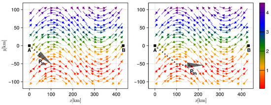
Consider a ship sailing in the tidal water area SA (see Figure 1):
- With the (tidal) stream (a horizontal flow of water caused by the rise and fall of the tide) given by the following velocity vector field:
- From point A to B, along the path/route:
- Under a specific control input (that corresponds to path ):
where denotes the ship course, is the ship relative speed, and and is the sailing area.
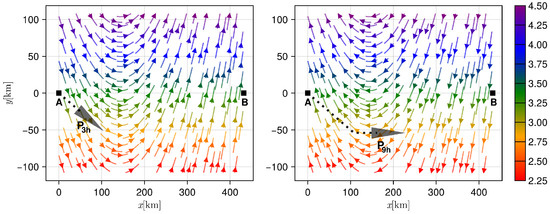
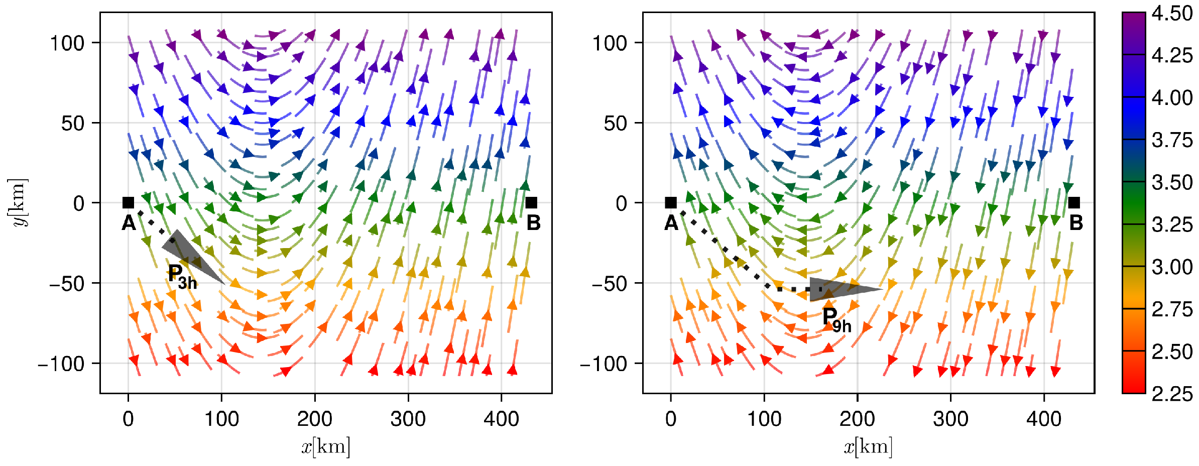
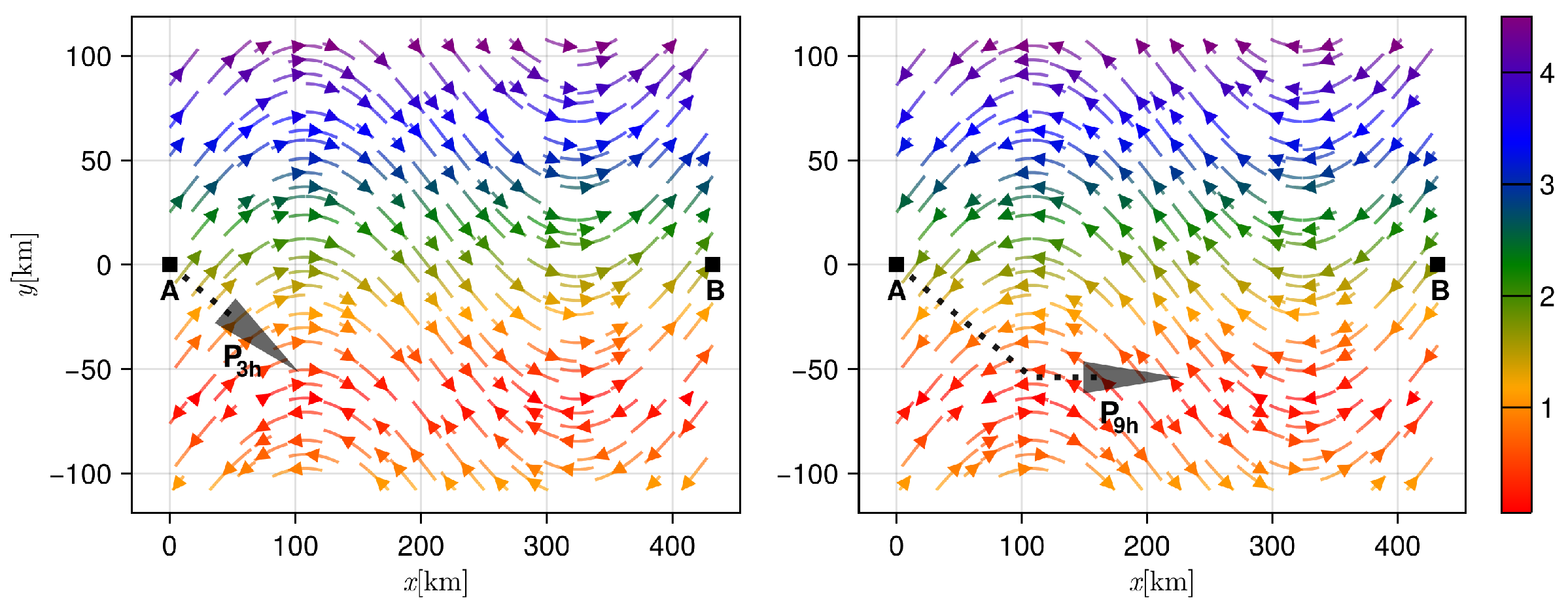
Figure 1.
Conceptual diagram of the first ship route () optimisation problem ([Prob1]) under consideration. (left) the tidal stream at time ; the ship—represented as the black triangle—sails with the current (as indicated by arrows). (right) the tidal stream at time ; the ship has to sail against the current. The colour bar shows absolute values, , of the tidal stream.
The route optimisation problem under consideration is to find a set of admissible control inputs —each causing the ship to follow an admissible path —which minimise in Pareto’s sense both the passage time (duration) and fuel consumption , i.e.,
Remark 1.
We assume that the values of both and can be found only through simulation (i.e., it is a black-box problem). The (simulation) model is described in Appendix A.
4. Proposed Solution
The approach presented in this paper is based on the following two main steps:
- Transformation of the continuous optimisation problem into a (discrete) search problem over a specially constructed graph;
- Application of the proposed optimal path search algorithm to find a good approximation of the set of Pareto optimal control input sequences:
Remark 2.
The sequence represents a continuous piecewise-linear sailing path (formed by the sequence of the graph edges that correspond to ), whilst is the sequence of relative ship speeds (along each linear path segment), which forms a piecewise-constant function.
The key elements of the proposed algorithm are as follows:
- A 3D-graph-based solution (design) space and the computational topology it generates (for dynamic programming (dp)-based local search);
- Adaptive Markov chain-based path generator (directing the search process);
- The search process augmented by the dp-based pruned local search.
They are discussed in the following subsections.
4.1. The Solution (Design) Space Representation
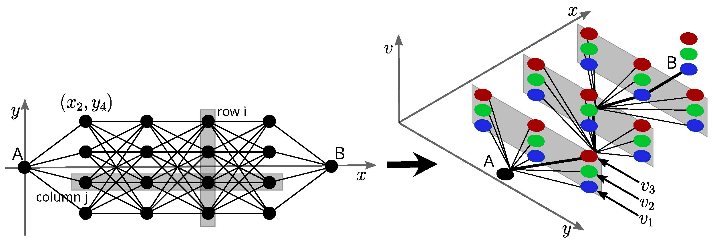
Discretisation of the original problem domain may be seen as a two-phase process [50]. In the first phase, we construct a multi-stage graph () that creates the “route space” (i.e., -space/spatial-dimension of , see Remark 2). In most instances, this graph is regular with equidistant nodes grouped in rows and columns: columns and () regular rows, plus two special (single-node) rows—one with point A and the other with point B (see Figure 2).
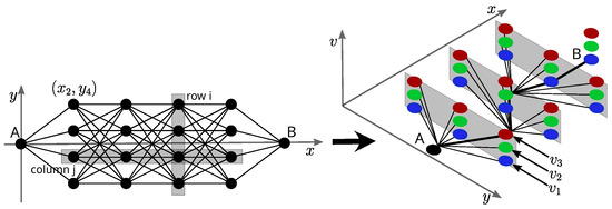
Figure 2.
Solution space representation. (left) multi-stage graph . (right) 3D-graph (for the sake of clarity of the drawing, the coordinate axes have been moved).
In the second phase, each node of (apart from the one corresponding to point A) is replicated times to add the -dimension to the solution space (of control inputs), which can be seen as an addition of the “third dimension” to . This new “3D-graph” () has the following traits [50]:
- Has nodes;
- Has edges;
- Represents different control input sequences. (trajectories).
Remark 3.
The piecewise-linear approximation of the ship route simplifies the problem significantly [50]. Instead of one complex, continuous two-dimensional problem, we have a series of simple one-dimensional subproblems—each corresponding to a single route segment only.
4.2. Path Generator
If we add to each node in layer of the solution space graph, the probabilities of reaching N from each node of the proceeding layer, the generation of the new path can be modelled as the -stage Markov decision process that starts at the final node B and goes backwards.
Remark 4.
The search graph enriched by the probability distributions, can be seen as the state space of the path-generating Markov chain.
The key elements of this generation process—which may be seen as the optimal path-search problem specific adaptation of the corresponding mechanisms of the Estimation of Distribution Algorithm (EDA)—are summarised below:
- At each node, the predecessor selection problem is two-dimensional (c and v are to be chosen) and discrete; hence, the corresponding joint probability distributions are represented as 2D-frequency tables ();
- The prior (initial) distributions are not uniform—they form a “gable roof shape” (with the marginal distribution of v being uniform, and the marginal distribution of c being triangular);
- Drawing is performed from the joint distribution, i.e., with a single draw, we obtain a pair of values ;
- Distribution adaptation is performed in two steps: first, the value corresponding to is increased by a predefined constant, i.e., , then, the distribution is “smoothed” locally (e.g., by weighted averaging).
4.3. dp-Based Pruned Local Search
Effective search algorithms often combine global and local techniques. The local search algorithm that we propose builds a search beam around every new path obtained from the generator. This process utilises the structure of the solution (design) space, which is a multi-stage graph (i.e., directed, acyclic, and layered); in this domain, the search beam is just a thin (“tube-shaped”) subgraph of that contains .
Having built this local search graph, we can apply dynamic programming to find—in a very effective way—all locally best new paths. This process can be additionally boosted by pruning because the evaluation of a single route segment can be aborted as soon as we know that it is not “promising” (this process can be based on any effective admissible heuristic; knowing the current approximation of the Pareto set helps as well). Since the cost of each route segment has to be obtained from simulation (it is unknown upfront), this improvement can be significant [50].
Remark 5.
The proposeddp-based local search—mainly due to its exploitation capabilities—is the key element of the algorithm: for every path obtained from the generator, it evaluates new paths (for instance, for , it corresponds to 129,140,162 new paths).
4.4. The Search Algorithm
The proposed multi-objective EDA-based algorithm with DP local search is presented in Algorithm 1. The input data include (initial search space with the prior distributions of the path-generating Markov chain pgmc), (tidal stream velocity vector field), (ship simulator), (predefined number of steps of the EDA), (predefined minimum number of new Pareto set candidates at each EDA step), and (predefined maximum number of draws—path generations—at each EDA step). The output of the algorithm is an approximation of the set of Pareto optimal control input sequences ().
The algorithm starts from initialising the set of Pareto optimal control input sequences (), the set of paths obtained from the path generator (), and the path generator pgmc (lines 1–3). The rest of the algorithm (lines 4–16) is iterated times.
Firstly, a new path is generated and added to the set of paths obtained from the path generator (lines 8–9). Next, dp-based pruned local search is performed “around” the generated path, and the resulting best paths found are added to the set of new Pareto set candidates (line 10), and the draws counter is incremented (line 11). The entire process is repeated until the minimum number of new candidates for the Pareto set has not been found and the maximum number of draws (generations of new paths) has not been reached (line 7).
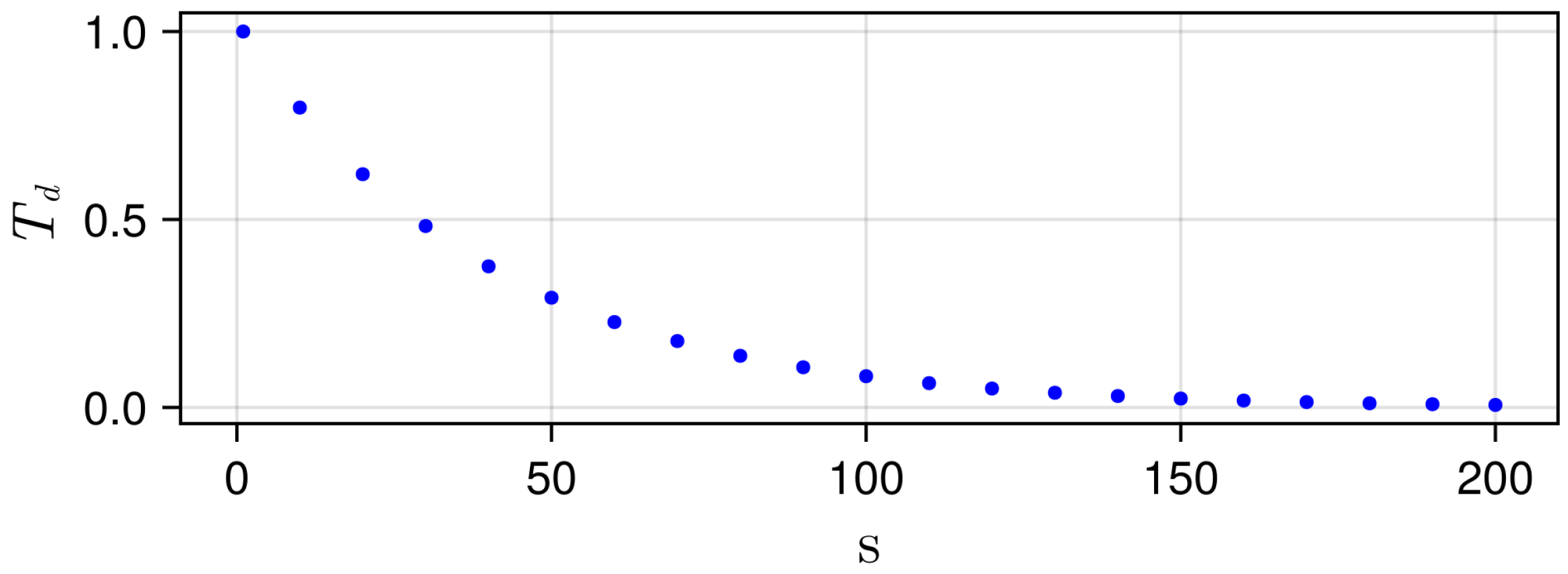
Subsequently, the approximation of Pareto set is updated using the set of new Pareto set candidates . Finally, the distributions of the path generator (pgmc) are updated (lines 13–16). If the number drawn with a uniform distribution on the interval (0,1) is greater than (see Figure 3), where:
then the distributions of the path generator pgmc are updated for all elements in the Pareto set (line 14). Otherwise, the distributions of the path generator are updated only for new elements of the Pareto set (line 16). This is to prevent premature convergence.
| Algorithm 1: Multi-objective ship route optimisation using estimation of distribution algorithm (EDA) with dp-based pruned local search. |
Input:
Output: —(good) approximation of the set of Pareto optimal control input sequences (see Equation (5)) |
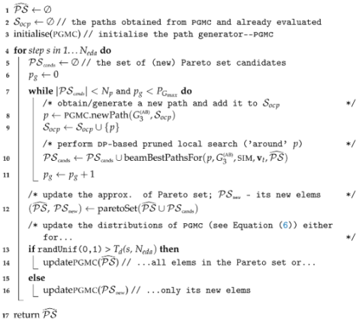 |
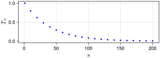
Figure 3.
function (see Equation (6)) shown for s = 1, 10, 20, …; .
Remark 6.
Algorithm 1 (average-case) time complexity is determined by the number of EDA steps (), the maximum number of path generations at each step (), and the average duration of single ab-path evaluation (), i.e.,
The space complexity formula, , arises from the solution space representation.
5. Results and Discussion
The experiments were aimed at verifying the efficacy of the proposed algorithm in the case of two problems ([Prob1] Figure 1, and [Prob2] Figure 4) of multi-objective ship routing in tidal waters (an example of a non-stationary environment).
The algorithms were implemented in Julia language [51]. A series of experiments was carried out using a MacBook Pro M2 with macOS 14.4.1. The obtained results are presented in Figure 5, Figure 6, Figure 7, Figure 8, Figure 9, Figure 10, Figure 11, Figure 12, Figure 13, Figure 14, Figure 15, Figure 16 and Figure 17.
5.1. Pareto Set Evolution (the Design Space Perspective)
In Figure 5, the found Pareto set for [Prob1] is presented. The graphs show relative (top) and absolute (bottom) ship velocity. In the charts, it can be seen that the final solution makes use of tidal streams, which is especially visible in the second half of the route, in the lower area of the map. As a result, the relative speed can be lower, which contributes to saving fuel and reducing travel time.
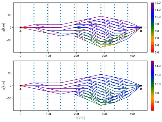
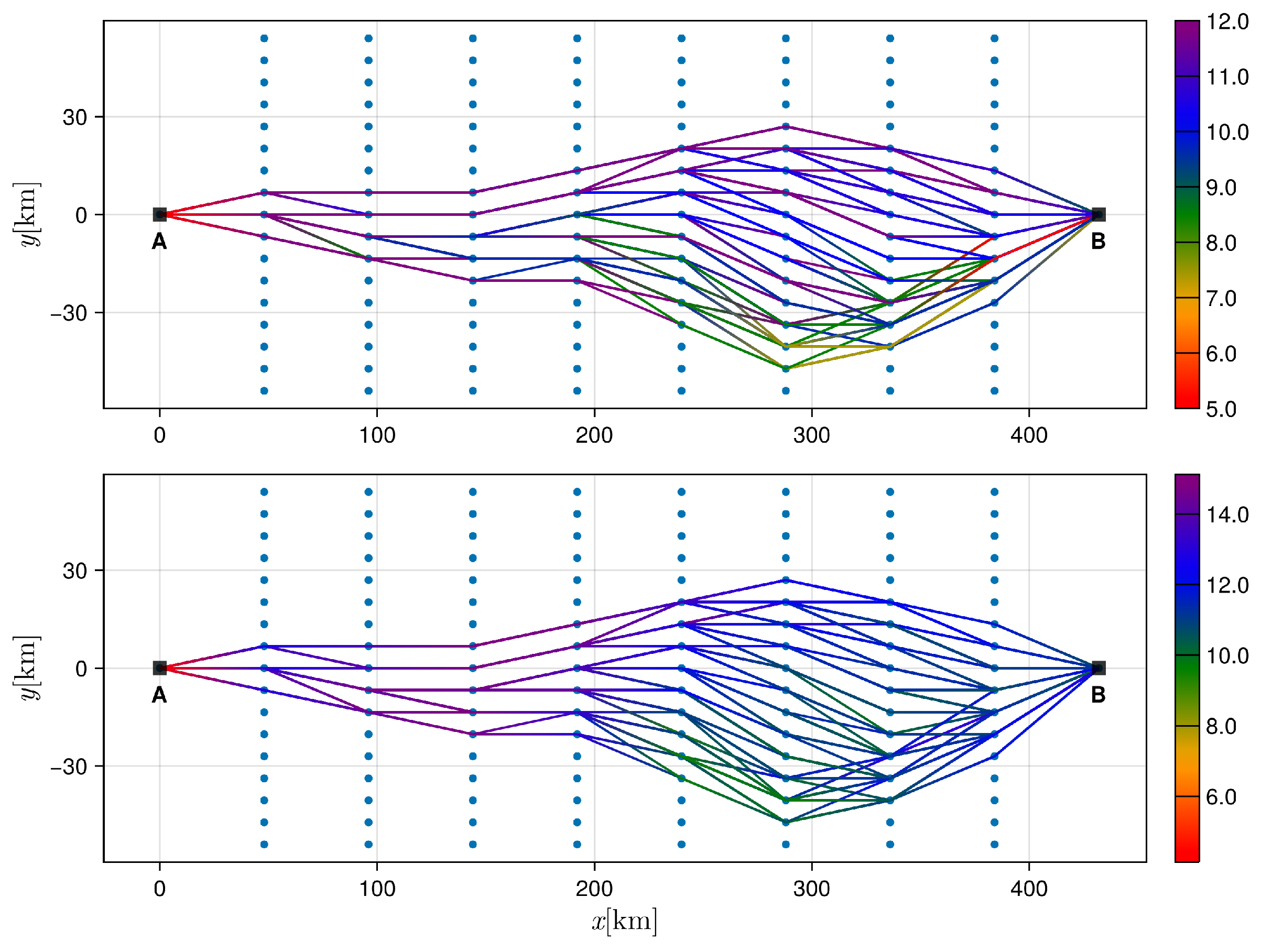
Figure 5.
[Prob1]: Pareto set (the paths in the design space) obtained with the proposed algorithm. (top) the colour of the path illustrates the relative ship velocity (STW, in m/s). (bottom) the colour of the path illustrates the absolute ship velocity (SOG).
Figure 5.
[Prob1]: Pareto set (the paths in the design space) obtained with the proposed algorithm. (top) the colour of the path illustrates the relative ship velocity (STW, in m/s). (bottom) the colour of the path illustrates the absolute ship velocity (SOG).
Figure 6 shows the evolution of the Pareto set in consecutive steps of the algorithm (1, 30, 100, and 200) for [Prob1]. The graphs show that in subsequent steps, the algorithm generates an increasingly larger Pareto set. It is especially visible in the lower part of the map area. This agrees with the results presented in Figure 5, where these routes made better use of the tidal stream, especially in the second half of the route. It is worth noting that none of the Pareto set snapshots contain the straight line solution (which seems to be an obvious one), which is caused by the action of the tidal stream.
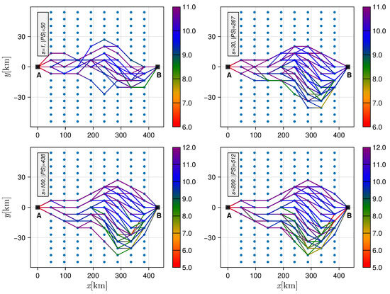

Figure 6.
[Prob1] Pareto set (the design space) in consecutive steps of the algorithm. (top left) step is 1, Pareto set size is 50. (top right) step is 30, Pareto set size is 267. (bottom left) step is 100, Pareto set size is 438. (bottom right) step is 200, Pareto set size is 512. The colour illustrates the relative speed (in m/s) of the ship.
Figure 7 shows the same process but for [Prob2].
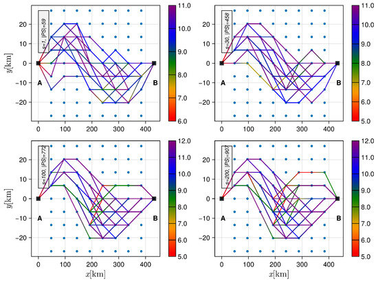
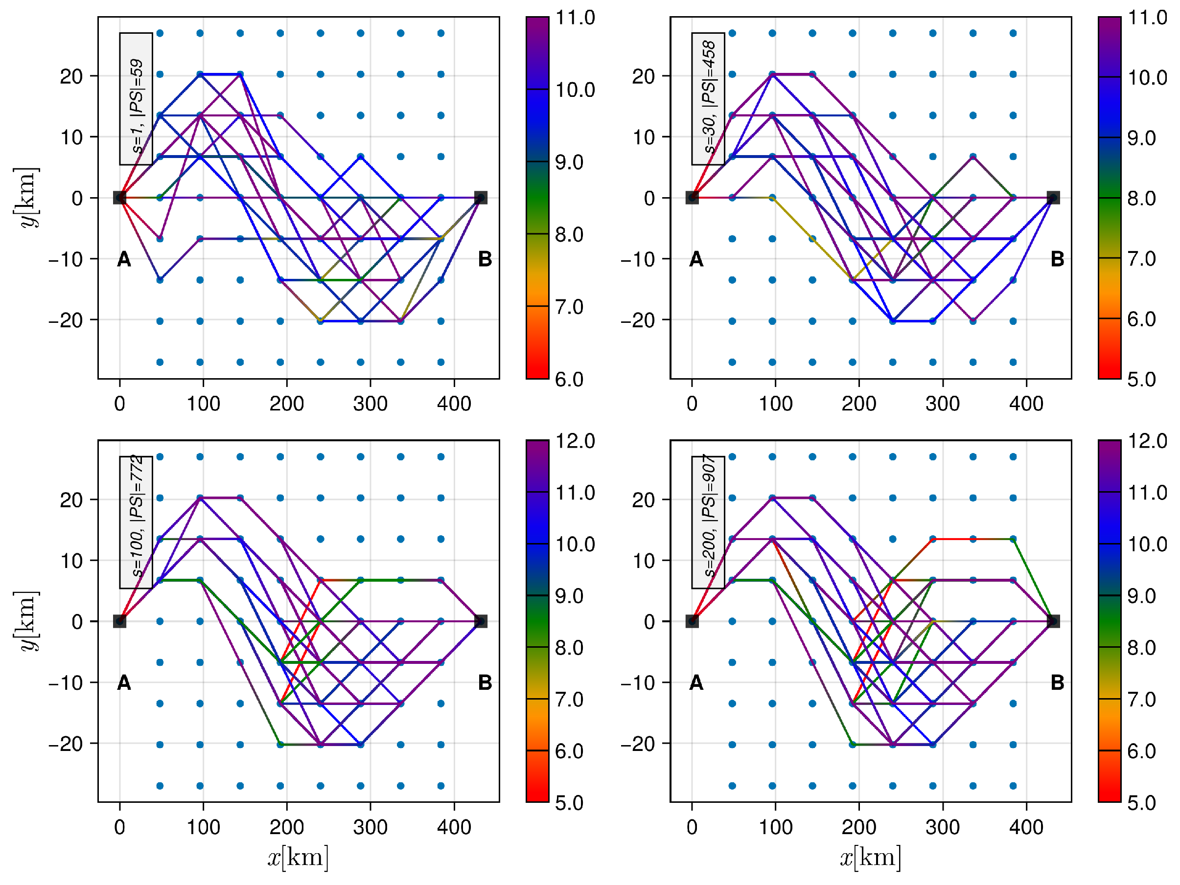
Figure 7.
[Prob2]: Pareto set (the design space) in consecutive steps of the algorithm. (top left) step is 1, Pareto set size is 59. (top right) step is 30, Pareto set size is 458. (bottom left) step is 100, Pareto set size is 772. (bottom right) step is 200, Pareto set size is 907. The colour illustrates the relative speed (in m/s) of the ship.
5.2. Pareto Front Evolution (The Criterion Space Perspective)
The Pareto front for [Prob1] in consecutive steps of the algorithm is shown in Figure 8. The colour used illustrates the quality of the front measured by the adapted Hypervolume (HV) metric [52]. With subsequent steps of the algorithm, it can be observed that the generated Pareto front is more and more numerous and its quality, measured by the value of the HV metric, is higher. At the same time, it can be noticed that from the very beginning of the algorithm’s operation, the front is very uniform and smooth, and there are no solutions that deviate significantly from it. Figure 9 shows the same process but for [Prob2].
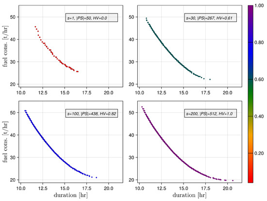
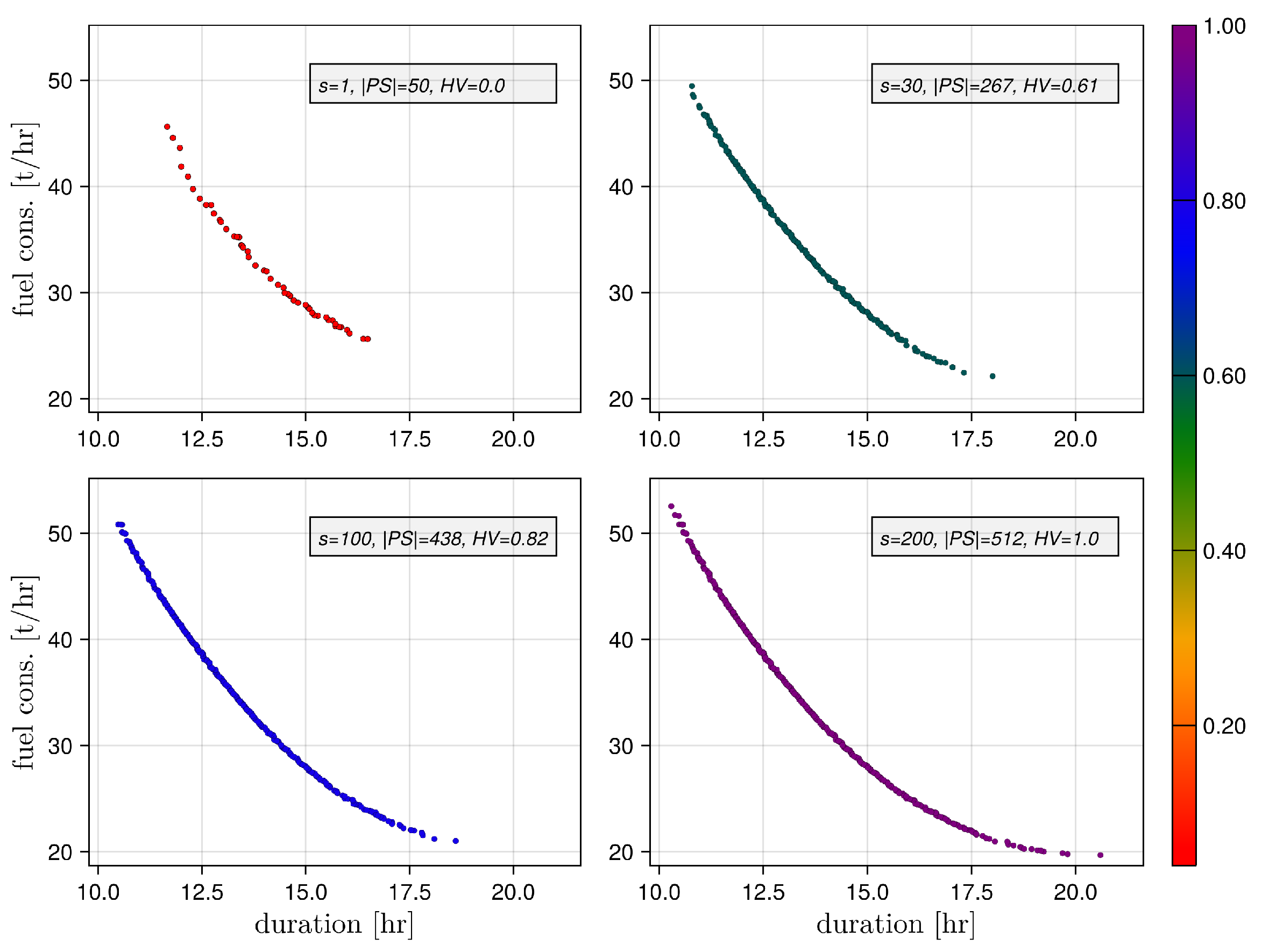
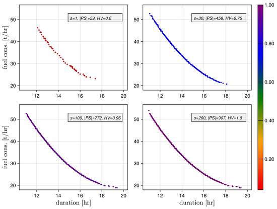

Figure 8.
[Prob1]: Pareto front (the criterion space) in consecutive steps of the algorithm. The colour of the Pareto front illustrates the value of the adapted Hypervolume (HV) metric. (top left) step is 1, Pareto set size is 50, and HV is 0.0. (top right) step is 30, Pareto set size is 267, and HV is 0.61. (bottom left) step is 100, Pareto set size is 438, and HV is 0.82. (bottom right) step is 200, Pareto set size is 512, and HV is 1.0.
Figure 9.
[Prob2]: Pareto front (the criterion space) in consecutive steps of the algorithm. The colour of Pareto front illustrates the value of adapted Hypervolume (HV) metric. (top left) step is 1, Pareto set size is 59, and HV is 0.0. (top right) step is 30, Pareto set size is 458, and HV is 0.75. (bottom left) step is 100, Pareto set size is 772, and HV is 0.96. (bottom right) step is 200, Pareto set size is 907, and HV is 1.0.
Figure 10 shows the Pareto front size and quality for [Prob1], measured by the adapted HV metric value, in consecutive steps of the algorithm. The graphs present two opposite views of the same process: the left graph emphasises the Pareto front size (with the colour representing HV metric value), whilst the right one highlights the HV metric value (the colour illustrates the front size). As the algorithm proceeds, the solutions on the Pareto front become more numerous and cover the front better and better. Because of this, the quality of the Pareto front measured by the HV metric increases. These results confirm the observations from Figure 8. At the same time, it should be emphasised that the algorithm maintains a high diversity of solutions on the Pareto front, which contributes to obtaining very good results, confirmed by the high value of the HV metric.
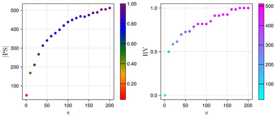
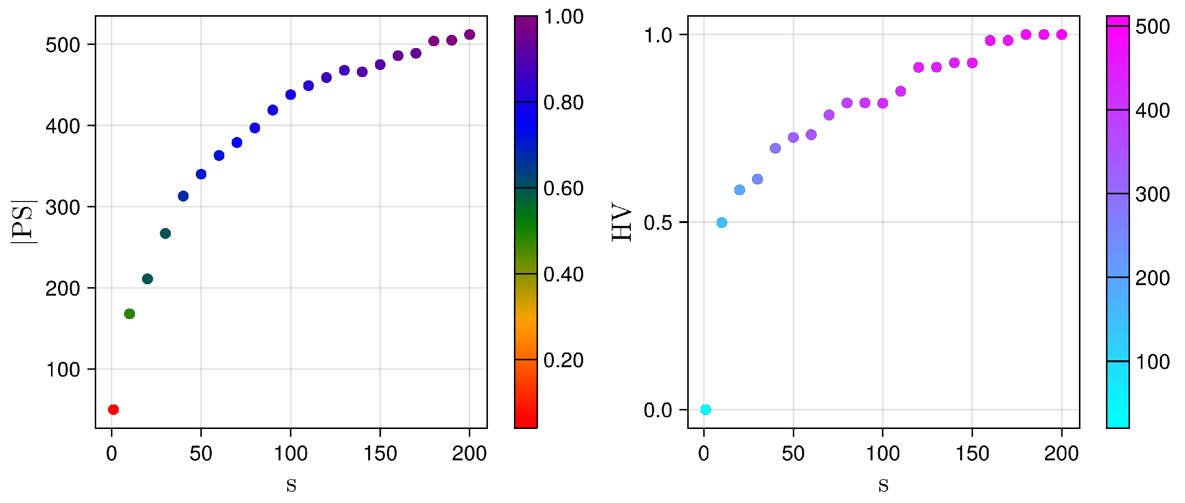
Figure 10.
[Prob1]: Pareto front size and quality (measured by the adapted HV metric value) in consecutive steps of the algorithm. (left) Pareto front size in consecutive steps, and the colour illustrates the HV metric value. (right) HV metric value, and the colour illustrates the Pareto front size.
Figure 11 shows the Pareto front size and quality for [Prob2]. As in the case of [Prob1] (Figure 10), in the consecutive steps of the algorithm, the solutions on the Pareto front become more numerous and cover the front better and better.

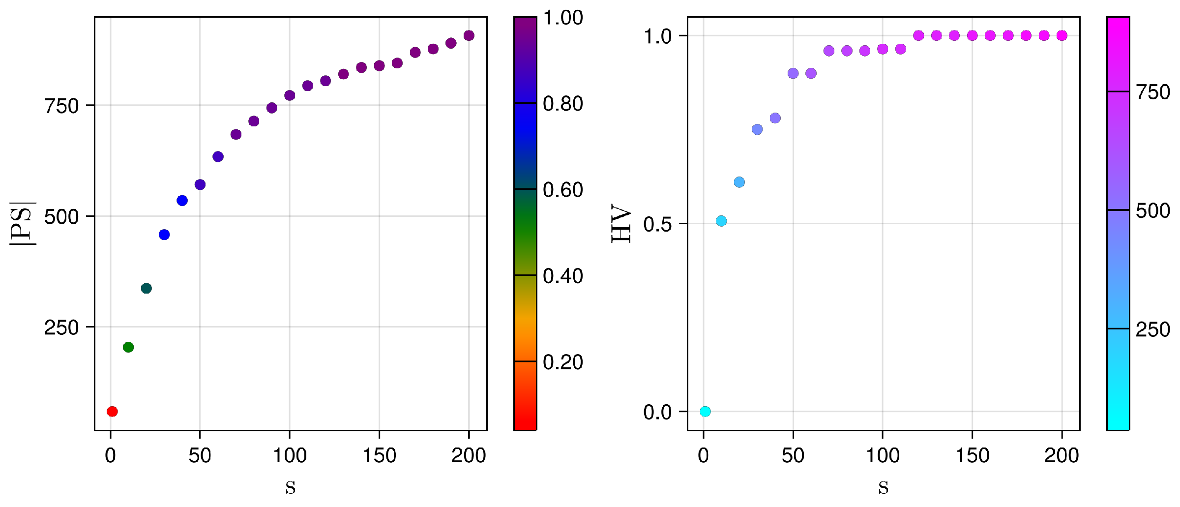
Figure 11.
[Prob2]: Pareto front size and quality (measured by the adapted HV metric value) in consecutive steps of the algorithm. (left) Pareto front size in consecutive steps, and the colour illustrates the HV metric value. (right) HV metric value, and the colour illustrates the Pareto front size.
5.3. Pareto Front Quality: The Impact of the Local Search
To quantify the impact of the local search on the overall performance of the optimisation algorithm, the numerical experiments described in Section 5.1 and Section 5.2 were repeated, but this time with the local search turned off. The corresponding results are shown in Figure 12, Figure 13, Figure 14, Figure 15, Figure 16 and Figure 17.
The paths forming (in the design space) the Pareto set for [Prob1], shown in Figure 12, differ significantly from those obtained from the full algorithm (see Figure 6): they are less numerous and cover different sailing areas (which means less effective use of the tidal stream). The same can be observed in Figure 7 and Figure 13, which correspond to [Prob2].
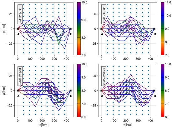
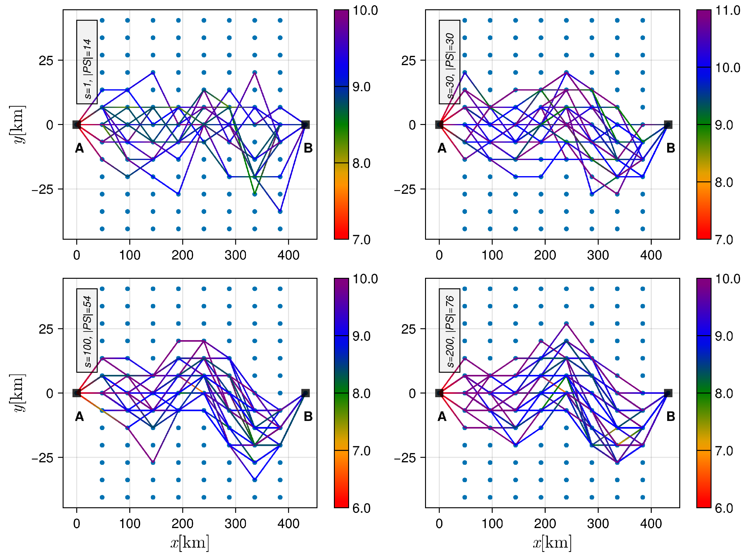
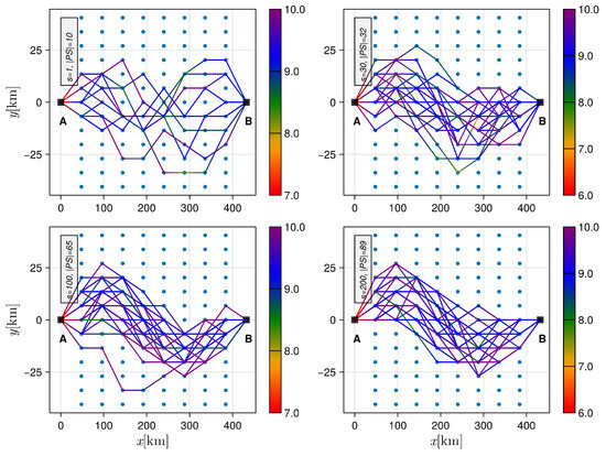

Figure 12.
[Prob1]: Pareto set (the design space) in consecutive steps of the algorithm without the local search. (top left) step is 1, and Pareto set size is 14. (top right) step is 30, and Pareto set size is 30. (bottom left) step is 100, and Pareto set size is 54. (bottom right) step is 200, and Pareto set size is 76. The colour illustrates the relative speed (in m/s) of the ship.
Figure 13.
[Prob2]: Pareto set (the design space) in consecutive steps of the algorithm without the local search. (top left) step is 1, and Pareto set size is 10. (top right) step is 30, and Pareto set size is 32. (bottom left) step is 100, and Pareto set size is 65. (bottom right) step is 200, and Pareto set size is 89. The colour illustrates the relative speed (in m/s) of the ship.
Figure 14 and Figure 15 present (in the criterion space) the evolution of the Pareto front for [Prob1] and [Prob2], respectively. Apart from being less numerous (which was mentioned above), the fronts are not as uniform and smooth as in the case of the full algorithm (see Figure 8 and Figure 9).
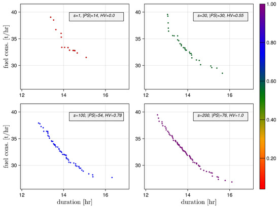


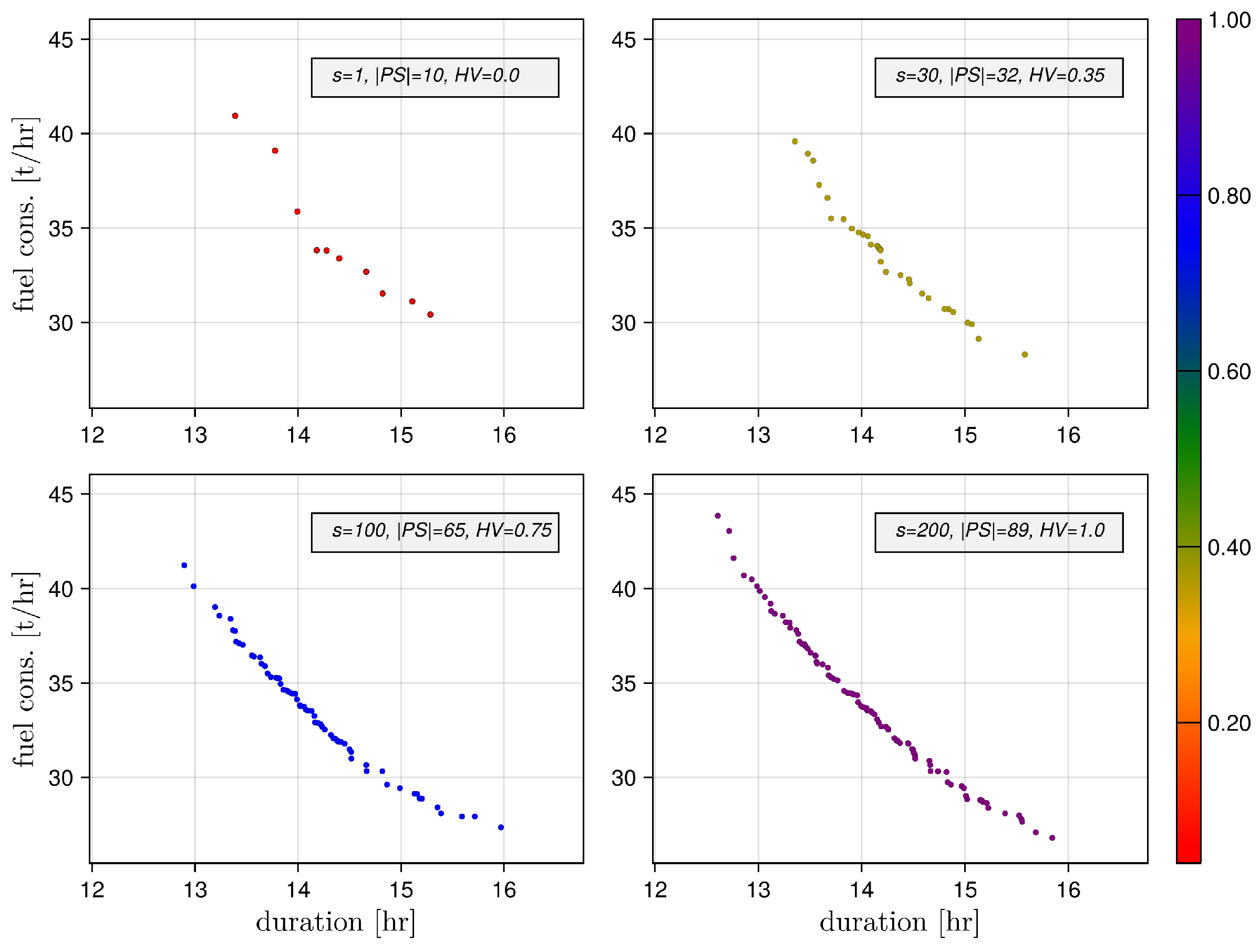
Figure 14.
[Prob1]: Pareto front (the criterion space) in consecutive steps of the algorithm without the local search. The colour of Pareto front illustrates the value of the adapted Hypervolume (HV) metric. (top left) step is 1, Pareto set size is 14, and HV is 0.0. (top right) step is 30, Pareto set size is 30, and HV is 0.55. (bottom left) step is 100, Pareto set size is 54, and HV is 0.78. (bottom right) step is 200, Pareto set size is 76, and HV is 1.0.
Figure 15.
[Prob2]: Pareto front (the criterion space) in consecutive steps of the algorithm without the local search. The colour of Pareto front illustrates the value of the adapted Hypervolume (HV) metric. (top left) step is 1, Pareto set size is 10, and HV is 0.0. (top right) step is 30, Pareto set size is 32, and HV is 0.35. (bottom left) step is 100, Pareto set size is 65, and HV is 0.75. (bottom right) step is 200, Pareto set size is 89, and HV is 1.0.
Figure 16 and Figure 17 show the size of the Pareto front and its quality in consecutive steps of the algorithm for [Prob1] and [Prob2], respectively. As before (see Figure 10 and Figure 11), the front quality is measured by the adapted HV metric value. This perspective gives a more detailed view of the search process—without the local algorithm support, it resembles a typical random search with “chaotic” changes in the size of the Pareto front; weaker exploitation of the solution space results in a smaller number of non-dominated solutions found.
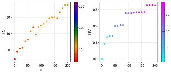
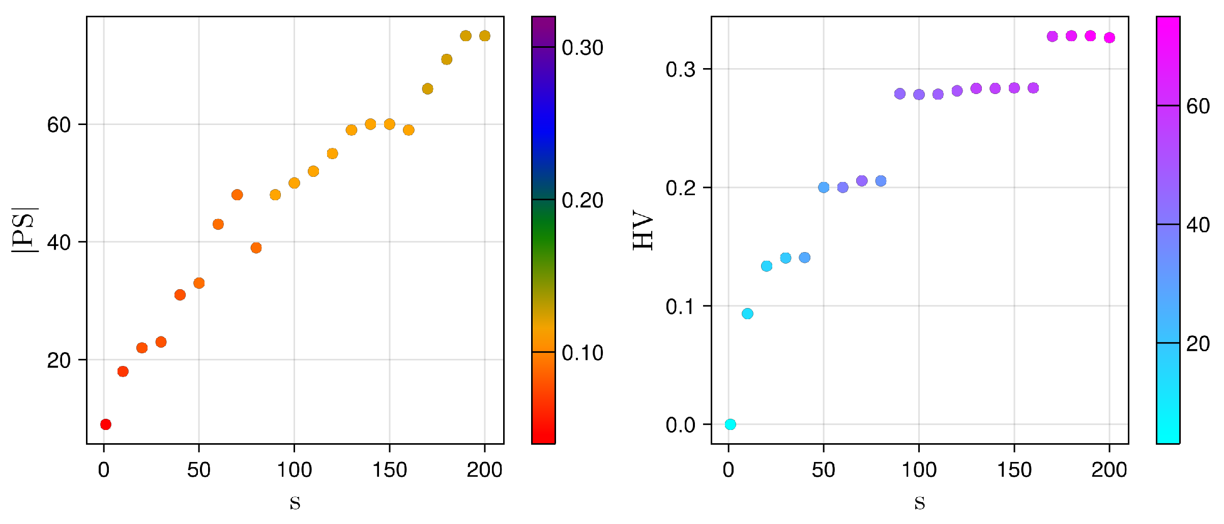

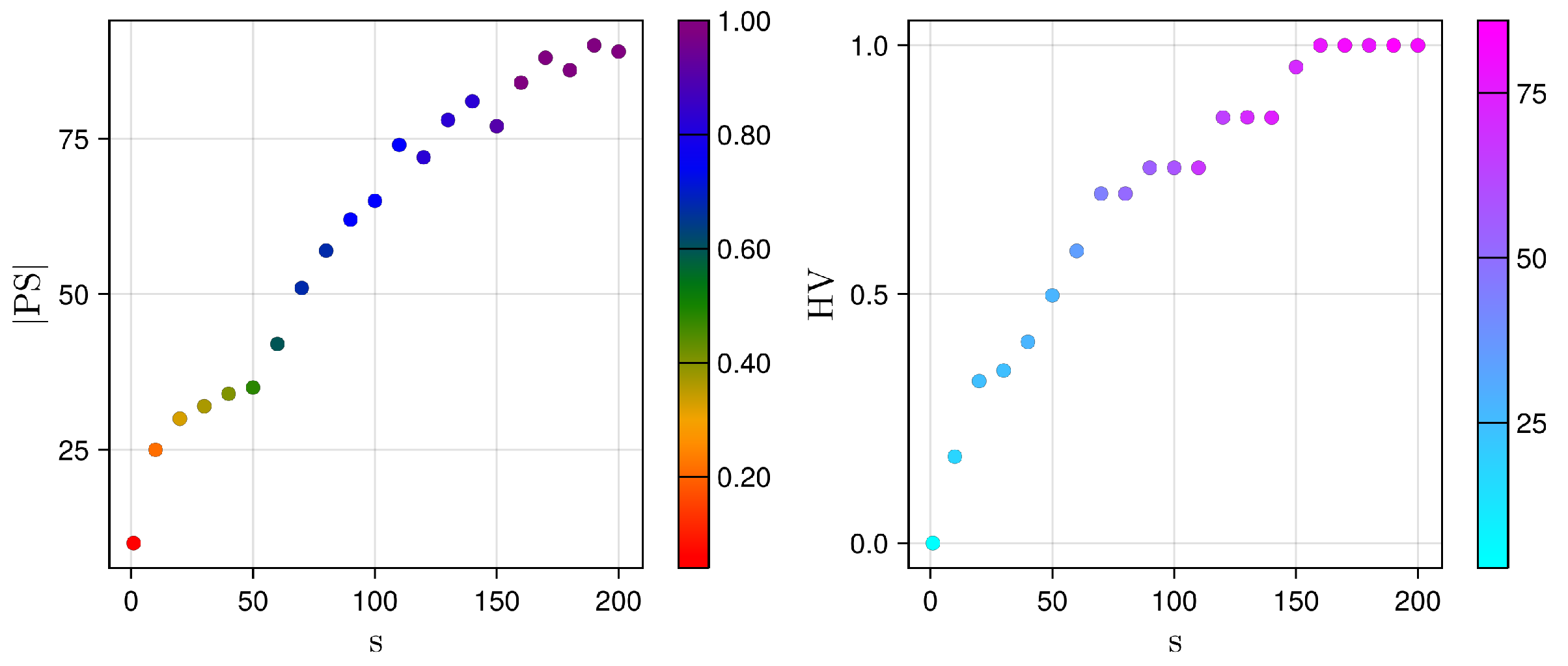
Figure 16.
[Prob1]: Pareto front size and quality (measured by the adapted HV metric value) in consecutive steps of the algorithm without the local search. (left) Pareto front size in consecutive steps, and the colour illustrates the HV metric value. (right) HV metric value, and the colour illustrates the Pareto front size.
Figure 17.
Same as Figure 16 but for [Prob2].
Figure 17.
Same as Figure 16 but for [Prob2].
5.4. Summary of the Results
Selected performance indicators of the proposed algorithm, investigated in Section 5.1, Section 5.2 and Section 5.3, are summarised in Table 2. In addition to the results related to the evolution of the Pareto set size and the Pareto front quality (measured by the metric), the table—in its last five columns—shows the significance of the local search, measured as a relative improvement in each of the performance indicators.
Table 2.
Summary of the results obtained by the proposed algorithm, both without and with the local search algorithm. The last part shows the percentage improvement in results when using local search. The individual symbols have the following meanings: (size of the Pareto front), (HV metric value), (minimum passage time), (minimum fuel consumption), and (-distance of the nearest point of the Pareto front from the criterion space origin).
In summary, the proposed algorithm shows a strong ability to find high-quality, diversified solutions to the multi-objective ship route optimisation problem in a non-stationary environment. The key element in achieving this proved to be the dynamic programming-based local search algorithm, whose application—thanks to its strong exploitation capabilities—improved the final result significantly: the Pareto set size increased more than five times, and the Pareto front quality just about doubled.
6. Conclusions
We have shown—on the example of optimisation of a ship’s route in tidal waters—an innovative adaptation of the estimation of distribution algorithm (EDA), intended for (simulation based) multi-objective optimal path planning in non-stationary environments.
The key elements of the proposed approach (apart from the specific design space) have been the adaptive Markov chain-based path generator (that directs the global search process) and the dynamic programming-based local search algorithm (that boosts—thanks to its exploitation capabilities—the global search process; see Table 2).
The presented experimental results indicate not only the high effectiveness of the proposed algorithm in finding very good quality (see Figure 10 and Figure 11) and diversified approximations (see Figure 8 and Figure 9) of optimal—in the Pareto sense—solutions but also a good exploration–exploitation balance of the search process.
The proposed algorithm can also be applied to other domains. As mentioned above, it can be seen as a framework for multi-objective optimal path planning (also simulation based) in non-stationary environments.
Future research work could concentrate on the following:
- Verification of the proposed algorithm with a more accurate ship simulator (based on ship dynamics);
- Verification of other (selected) existing meta-heuristics as the global search process engines;
- The search algorithm hyper-parameters tuning, combined with sensitivity analysis;
- The parallelisation of the algorithm;
- The use of other types of surrogate models.
Author Contributions
Conceptualisation, R.D. (Roman Dębski); Data curation, R.D. (Roman Dębski); Formal analysis, R.D. (Roman Dębski); Funding acquisition, R.D. (Rafał Dreżewski); Investigation, R.D. (Roman Dębski) and R.D. (Rafał Dreżewski); Methodology, R.D. (Roman Dębski); Project administration, R.D. (Roman Dębski); Resources, R.D. (Roman Dębski); Software, R.D. (Roman Dębski); Supervision, R.D. (Roman Dębski) and R.D. (Rafał Dreżewski); Validation, R.D. (Roman Dębski); Visualisation, R.D. (Roman Dębski) and R.D. (Rafał Dreżewski); Writing—original draft, R.D. (Roman Dębski) and R.D. (Rafał Dreżewski); Writing—review and editing, R.D. (Roman Dębski) and R.D. (Rafał Dreżewski). All authors have read and agreed to the published version of the manuscript.
Funding
This research was supported by the Polish Ministry of Science and Higher Education funds assigned to AGH University of Krakow.
Institutional Review Board Statement
Not applicable.
Informed Consent Statement
Not applicable.
Data Availability Statement
The original contributions presented in the study are included in the article, further inquiries can be directed to the corresponding author.
Conflicts of Interest
The authors declare no conflicts of interest.
Appendix A. The Simulation Model
- Without loss of generality (the simulator—independently of its complexity—is treated by the optimisation algorithm as a black-box), we define only the kinematic model of a ship, which describes the motion of the ship without consideration of forces (an example of a more complex model can be found, for instance, in [50]).
- The optimisation problem under consideration (see Section 3) has two objectives: the passage time and the corresponding fuel consumption are to be minimised. They are defined in the following way:
- (a)
- Passage time (duration), calculated as a sum of passage times for each linear path segment, r:
- (b)
- Fuel consumption (total), as above—accumulated over all segments:
where () is the number of segments forming a single ab-path, is the length of the r-th segment, is the number of subsegments used to approximate the integral , is the absolute speed (SOG—Speed Over the Ground) of the ship (along the r-th linear segment), and is the speed of the ship relative to the water (STW—Speed Through Water). - The ship absolute speed (SOG) depends on the tidal stream (typically given in the form of a vector field), which in the simulations is assumed to be as follows (see Figure 1 and Figure 4):where:
- (a)
- (b)
Finally, the ship absolute speed (along the given path segment ) is defined as follows:where is the angle (slope) of and - In addition, we assume the following:
- (a)
- Each ab-path is a continuous piecewise-linear function (formed by the sequence of the corresponding graph edges).
- (b)
- Each control input sequence is a piecewise-constant function (constant along each linear path segment).
References
- United Nations Conference on Trade and Development (UNCTAD). Review of Maritime Transport; UNCTAD: Geneva, Switzerland, 2022. [Google Scholar]
- Shao, W.; Zhou, P.; Thong, S.K. Development of a novel forward dynamic programming method for weather routing. J. Mar. Sci. Technol. 2012, 17, 239–251. [Google Scholar] [CrossRef]
- Szlapczynska, J.; Szlapczynski, R. Preference-based evolutionary multi-objective optimization in ship weather routing. Appl. Soft Comput. 2019, 84, 105742. [Google Scholar] [CrossRef]
- Du, W.; Li, Y.; Zhang, G.; Wang, C.; Zhu, B.; Qiao, J. Energy saving method for ship weather routing optimization. Ocean Eng. 2022, 258, 111771. [Google Scholar] [CrossRef]
- Gunawan; Utomo, A.; Pambudi, G.; Hamada, K.; Yanuar. Optimization of Shipping Routes for Container Ships from Indonesia to the Asia-Pacific Using Heuristic Algorithms. J. Mar. Sci. Eng. 2023, 11, 1360. [Google Scholar] [CrossRef]
- Chung, S.H. Applications of smart technologies in logistics and transport: A review. Transp. Res. Part E Logist. Transp. Rev. 2021, 153, 102455. [Google Scholar] [CrossRef]
- Khan, W.A.; Chung, S.; Awan, M.U.; Wen, X. Machine learning facilitated business intelligence (Part II): Neural networks optimization techniques and applications. Ind. Manag. Data Syst. 2020, 120, 128–163. [Google Scholar] [CrossRef]
- Orosa, J.A.; Pérez-Canosa, J.M.; Pérez-Castelo, F.J.; Durán-Grados, V. Research on the Improvement of Safety Navigation Based on the Shipmaster’s Control of Ship Navigational Parameters When Sailing in Different Sea State Conditions. Appl. Sci. 2023, 13, 4486. [Google Scholar] [CrossRef]
- Du, W.; Li, Y.; Zhang, G.; Wang, C.; Chen, P.; Qiao, J. Estimation of ship routes considering weather and constraints. Ocean Eng. 2021, 228, 108695. [Google Scholar] [CrossRef]
- Wang, X.; Zhao, X.; Wang, G.; Wang, Q.; Feng, K. Weather Route Optimization Method of Unmanned Ship Based on Continuous Dynamic Optimal Control. Sustainability 2022, 14, 2165. [Google Scholar] [CrossRef]
- Wang, H.; Mao, W.; Eriksson, L. A Three-Dimensional Dijkstra’s algorithm for multi-objective ship voyage optimization. Ocean Eng. 2019, 186, 106131. [Google Scholar] [CrossRef]
- Hagiwara, H.; Spaans, J.A. Practical Weather Routing of Sail-assisted Motor Vessels. J. Navig. 1987, 40, 96–119. [Google Scholar] [CrossRef]
- Spaans, J.A.; Stoter, P.H. New developments in ship weather routing. Navigation 1995, 43, 95–106. [Google Scholar]
- Bijlsma, S.J. On the Applications of Optimal Control Theory and Dynamic Programming in Ship Routing. Navigation 2002, 49, 71–80. [Google Scholar] [CrossRef]
- Padhy, C.; Sen, D.; Bhaskaran, P. Application of wave model for weather routing of ships in the North Indian Ocean. Nat. Hazards 2008, 44, 373–385. [Google Scholar] [CrossRef]
- Szlapczynska, J.; Smierzchalski, R. Multicriteria Optimisation in Weather Routing. TransNav Int. J. Mar. Navig. Saf. Sea Transp. 2009, 3, 393–400. [Google Scholar] [CrossRef]
- Maki, A.; Akimoto, Y.; Nagata, Y.; Kobayashi, S.; Kobayashi, E.; Shiotani, S.; Ohsawa, T.; Umeda, N. A new weather-routing system that accounts for ship stability based on a real-coded genetic algorithm. J. Mar. Sci. Technol. 2011, 16, 311–322. [Google Scholar] [CrossRef]
- Lin, Y.H.; Fang, M.C.; Yeung, R.W. The optimization of ship weather-routing algorithm based on the composite influence of multi-dynamic elements. Appl. Ocean Res. 2013, 43, 184–194. [Google Scholar] [CrossRef]
- Kytariolou, A.; Themelis, N. Optimized Route Planning under the Effect of Hull and Propeller Fouling and Considering Ocean Currents. J. Mar. Sci. Eng. 2023, 11, 828. [Google Scholar] [CrossRef]
- Zis, T.P.; Psaraftis, H.N.; Ding, L. Ship weather routing: A taxonomy and survey. Ocean Eng. 2020, 213, 107697. [Google Scholar] [CrossRef]
- Li, Y.; Cui, J.; Zhang, X.; Yang, X. A Ship Route Planning Method under the Sailing Time Constraint. J. Mar. Sci. Eng. 2023, 11, 1242. [Google Scholar] [CrossRef]
- Jia, H.; Yang, Y.; An, J.; Fu, R. A Ship Trajectory Prediction Model Based on Attention-BILSTM Optimized by the Whale Optimization Algorithm. Appl. Sci. 2023, 13, 4907. [Google Scholar] [CrossRef]
- Mao, W.; Rychlik, I.; Wallin, J.; Storhaug, G. Statistical models for the speed prediction of a container ship. Ocean Eng. 2016, 126, 152–162. [Google Scholar] [CrossRef]
- Veneti, A.; Makrygiorgos, A.; Konstantopoulos, C.; Pantziou, G.; Vetsikas, I.A. Minimizing the fuel consumption and the risk in maritime transportation: A bi-objective weather routing approach. Comput. Oper. Res. 2017, 88, 220–236. [Google Scholar] [CrossRef]
- Szlapczynska, J. Multiobjective Approach to Weather Routing. TransNav Int. J. Mar. Navig. Saf. Sea Transp. 2007, 1, 273–278. [Google Scholar]
- Hinnenthal, J.; Clauss, G. Robust Pareto-optimum routing of ships utilising deterministic and ensemble weather forecasts. Ships Offshore Struct. 2010, 5, 105–114. [Google Scholar] [CrossRef]
- Zhao, W.; Wang, Y.; Zhang, Z.; Wang, H. Multicriteria Ship Route Planning Method Based on Improved Particle Swarm Optimization—Genetic Algorithm. J. Mar. Sci. Eng. 2021, 9, 357. [Google Scholar] [CrossRef]
- Zhao, S.; Zhao, S. Ship Global Traveling Path Optimization via a Novel Non-Dominated Sorting Genetic Algorithm. J. Mar. Sci. Eng. 2024, 12, 485. [Google Scholar] [CrossRef]
- Larrañaga, P.; Lozano, J.A. (Eds.) Estimation of Distribution Algorithms: A New Tool for Evolutionary Computation, 2nd ed.; Springer: New York, NY, USA, 2012. [Google Scholar]
- Li, Y.; Yang, Q.; Gao, X.D.; Lu, Z.Y.; Zhang, J. A layered learning estimation of distribution algorithm. In Proceedings of the Genetic and Evolutionary Computation Conference Companion, Boston, MA, USA, 9–13 July 2022; pp. 399–402. [Google Scholar] [CrossRef]
- Ceberio, J.; Irurozki, E.; Mendiburu, A.; Lozano, J.A. A review on estimation of distribution algorithms in permutation-based combinatorial optimization problems. Prog. Artif. Intell. 2012, 1, 103–117. [Google Scholar] [CrossRef]
- Krejca, M.S. Theoretical Analyses of Univariate Estimation-of-Distribution Algorithms. Ph.D. Thesis, University of Potsdam, Potsdam, Germany, 2019. [Google Scholar] [CrossRef]
- Yang, Q.; Chen, W.N.; Zhang, J. Probabilistic Multimodal Optimization. In Metaheuristics for Finding Multiple Solutions; Preuss, M., Epitropakis, M.G., Li, X., Fieldsend, J.E., Eds.; Springer International Publishing: Cham, Switzerland, 2021; pp. 191–228. [Google Scholar] [CrossRef]
- Grahl, J.; Bosman, P.A.; Rothlauf, F. The correlation-triggered adaptive variance scaling IDEA. In Proceedings of the 8th Annual Conference on Genetic and Evolutionary Computation, New York, NY, USA, 8–12 July 2006; pp. 397–404. [Google Scholar] [CrossRef]
- Bosman, P.A.N.; Grahl, J.; Rothlauf, F. SDR: A better trigger for adaptive variance scaling in normal EDAs. In Proceedings of the 9th Annual Conference on Genetic and Evolutionary Computation, New York, NY, USA, 7–11 July 2007; pp. 492–499. [Google Scholar] [CrossRef]
- Cai, Y.; Sun, X.; Xu, H.; Jia, P. Cross entropy and adaptive variance scaling in continuous EDA. In Proceedings of the 9th Annual Conference on Genetic and Evolutionary Computation, New York, NY, USA, 7–11 July 2007; pp. 609–616. [Google Scholar] [CrossRef]
- Yang, P.; Tang, K.; Lu, X. Improving Estimation of Distribution Algorithm on Multimodal Problems by Detecting Promising Areas. IEEE Trans. Cybern. 2015, 45, 1438–1449. [Google Scholar] [CrossRef]
- Huang, S.; Jiang, H. Multimodal estimation of distribution algorithm based on cooperative clustering strategy. In Proceedings of the 2018 Chinese Control And Decision Conference (CCDC), Shenyang, China, 9–11 June 2018; pp. 5297–5302. [Google Scholar] [CrossRef]
- Khan, N. Bayesian Optimization Algorithms for Multiobjective and Hierarchically Difficult Problems. Ph.D. Thesis, University of Illinois at Urbana-Champaign, Urbana, IL, USA, 2003. [Google Scholar]
- Laumanns, M.; Ocenasek, J. Bayesian optimization algorithms for multi-objective optimization. In Proceedings of the 7th International Conference on Parallel Problem Solving from Nature, Granada, Spain, 7–11 September 2002; Springer: Berlin/Heidelberg, Germany, 2002; pp. 298–307. [Google Scholar]
- Pelikan, M.; Sastry, K.; Goldberg, D.E. Multiobjective Estimation of Distribution Algorithms. In Scalable Optimization via Probabilistic Modeling; Pelikan, M., Sastry, K., CantúPaz, E., Eds.; Springer: Berlin/Heidelberg, Germany, 2006; pp. 223–248. [Google Scholar] [CrossRef]
- Karshenas, H.; Santana, R.; Bielza, C.; Larrañaga, P. Multiobjective Estimation of Distribution Algorithm Based on Joint Modeling of Objectives and Variables. IEEE Trans. Evol. Comput. 2014, 18, 519–542. [Google Scholar] [CrossRef]
- Jiang, M.; Qiu, L.; Huang, Z.; Yen, G.G. Dynamic Multi-Objective Estimation of Distribution Algorithm Based on Domain Adaptation and Nonparametric Estimation. Inf. Sci. 2018, 435, 203–223. [Google Scholar] [CrossRef]
- Botello-Aceves, S.; Hernandez-Aguirre, A.; Valdez, S.I. The Directed Multi-Objective Estimation Distribution Algorithm (D-MOEDA). Math. Comput. Simul. 2023, 214, 334–351. [Google Scholar] [CrossRef]
- Yang, P.; Tang, K.; Lozano, J.A. Estimation of Distribution Algorithms based Unmanned Aerial Vehicle path planner using a new coordinate system. In Proceedings of the 2014 IEEE Congress on Evolutionary Computation (CEC), Beijing, China, 6–11 July 2014; pp. 1469–1476. [Google Scholar] [CrossRef]
- Shirazi, A. Adaptive Estimation of Distribution Algorithms for Low-Thrust Trajectory Optimization. J. Spacecr. Rocket. 2023, 60, 1–12. [Google Scholar] [CrossRef]
- Zhang, Q.; Sun, J.; Tsang, E.; Ford, J. Estimation of Distribution Algorithm with 2-opt Local Search for the Quadratic Assignment Problem. In Towards a New Evolutionary Computation: Advances in the Estimation of Distribution Algorithms; Lozano, J.A., Larrañaga, P., Inza, I., Bengoetxea, E., Eds.; Springer: Berlin/Heidelberg, Germany, 2006; pp. 281–292. [Google Scholar] [CrossRef]
- Jarboui, B.; Eddaly, M.; Siarry, P. An estimation of distribution algorithm for minimizing the total flowtime in permutation flowshop scheduling problems. Comput. Oper. Res. 2009, 36, 2638–2646. [Google Scholar] [CrossRef]
- Du, Y.; Li, J.Q.; Luo, C.; Meng, L.L. A hybrid estimation of distribution algorithm for distributed flexible job shop scheduling with crane transportations. Swarm Evol. Comput. 2021, 62, 100861. [Google Scholar] [CrossRef]
- Dębski, R.; Dreżewski, R. Surrogate-Assisted Ship Route Optimisation. In Proceedings of the International Conference on Computational Science, Prague, Czech Republic, 3–5 July 2023; Springer: Cham, Switzerland, 2023; pp. 395–409. [Google Scholar] [CrossRef]
- Bezanson, J.; Edelman, A.; Karpinski, S.; Shah, V.B. Julia: A fresh approach to numerical computing. SIAM Rev. 2017, 59, 65–98. [Google Scholar] [CrossRef]
- Audet, C.; Bigeon, J.; Cartier, D.; Le Digabel, S.; Salomon, L. Performance indicators in multiobjective optimization. Eur. J. Oper. Res. 2021, 292, 397–422. [Google Scholar] [CrossRef]
Disclaimer/Publisher’s Note: The statements, opinions and data contained in all publications are solely those of the individual author(s) and contributor(s) and not of MDPI and/or the editor(s). MDPI and/or the editor(s) disclaim responsibility for any injury to people or property resulting from any ideas, methods, instructions or products referred to in the content. |
© 2024 by the authors. Licensee MDPI, Basel, Switzerland. This article is an open access article distributed under the terms and conditions of the Creative Commons Attribution (CC BY) license (https://creativecommons.org/licenses/by/4.0/).