

Air Quality Predictions through Mathematical Modeling for Iron Ore Mine Project

Abstract
:1. Introduction
- Survey of the various air quality prediction models (AQMs) and selection of the most suitable model for predicting air quality impacts for an iron ore mine project for short-term area sources and a flat terrain, while accounting for the actual field conditions.
- To quantify SPM and PM10 in the dry season during the construction phase and model the same with the established model and continue monitoring during operation phases.
- To propose mitigation measures based on simulations to minimize air quality impacts based on AQM predictions and their implementation for compliance with environmental standards during operation phase.
- To evaluate air quality trends over distance and the variability of SPM and PM10 using exploratory analysis, while evaluating the effectiveness of implemented mitigation strategies.
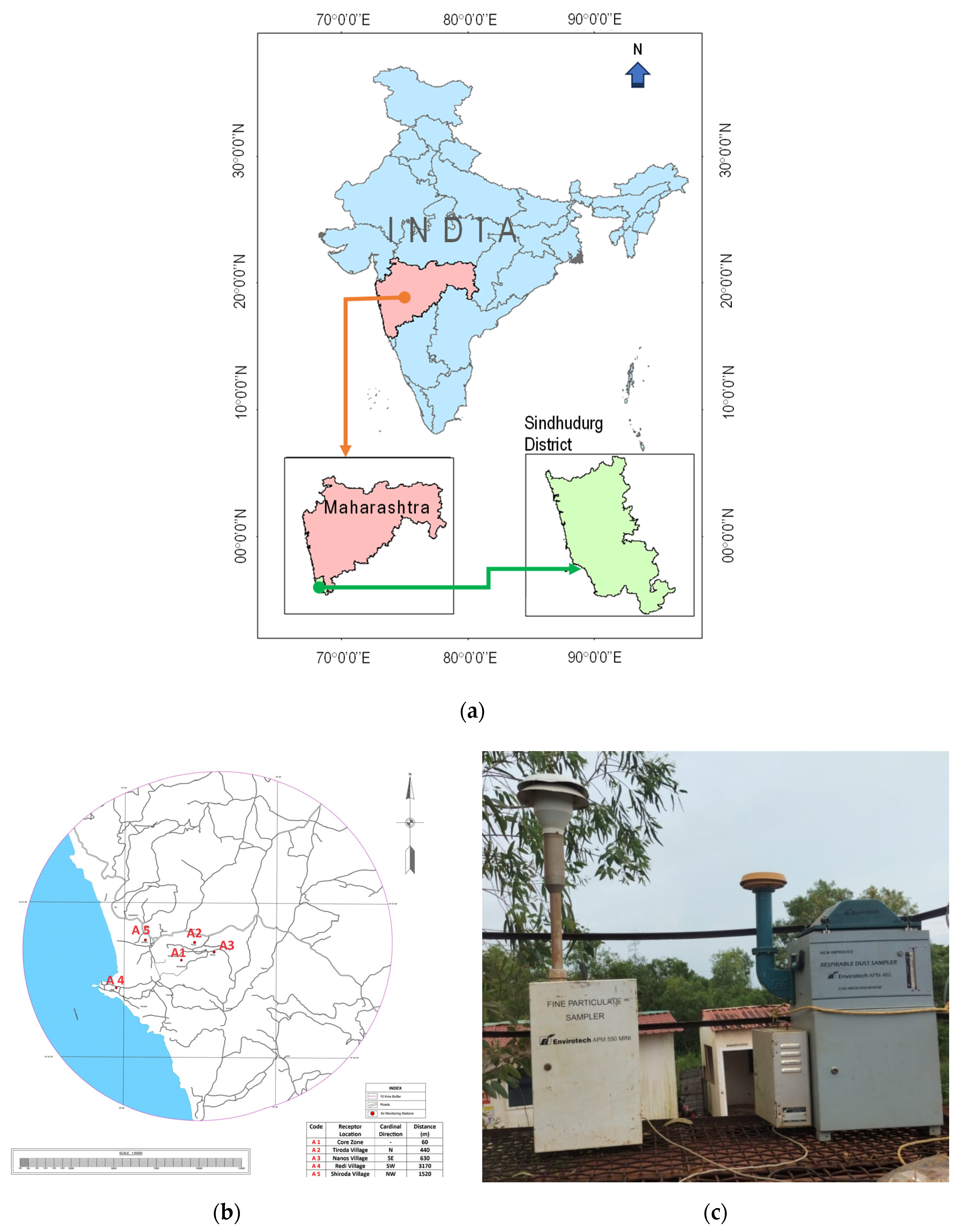
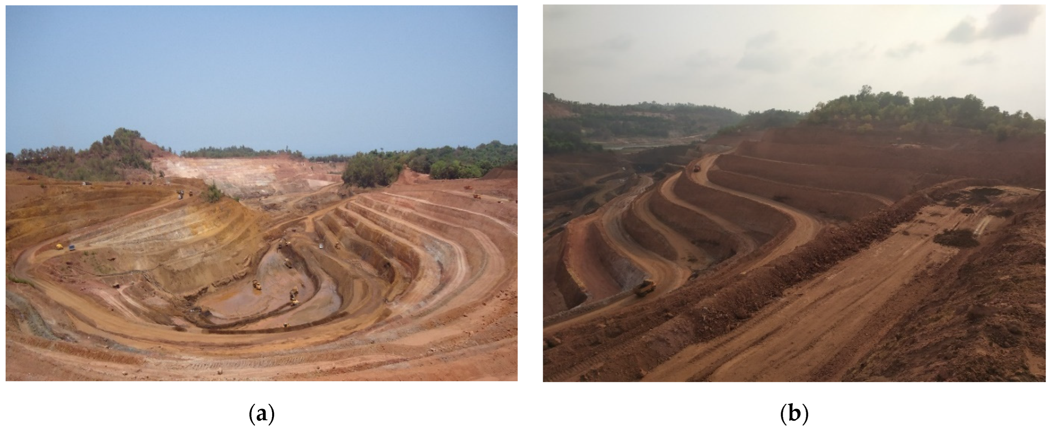
2. Study Area
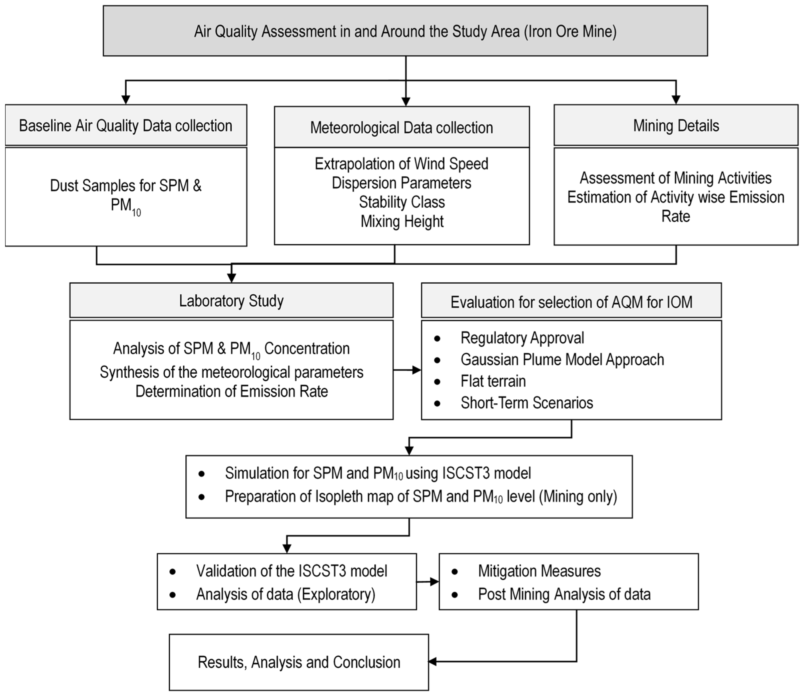
3. Methodology
3.1. Data Acquisition and Compilation
3.2. Survey of the Air Quality Models
3.3. Air Quality Assessment
3.3.1. Impact on Air Quality during Construction Phase
3.3.2. Impact on Air Quality during Operation Phase
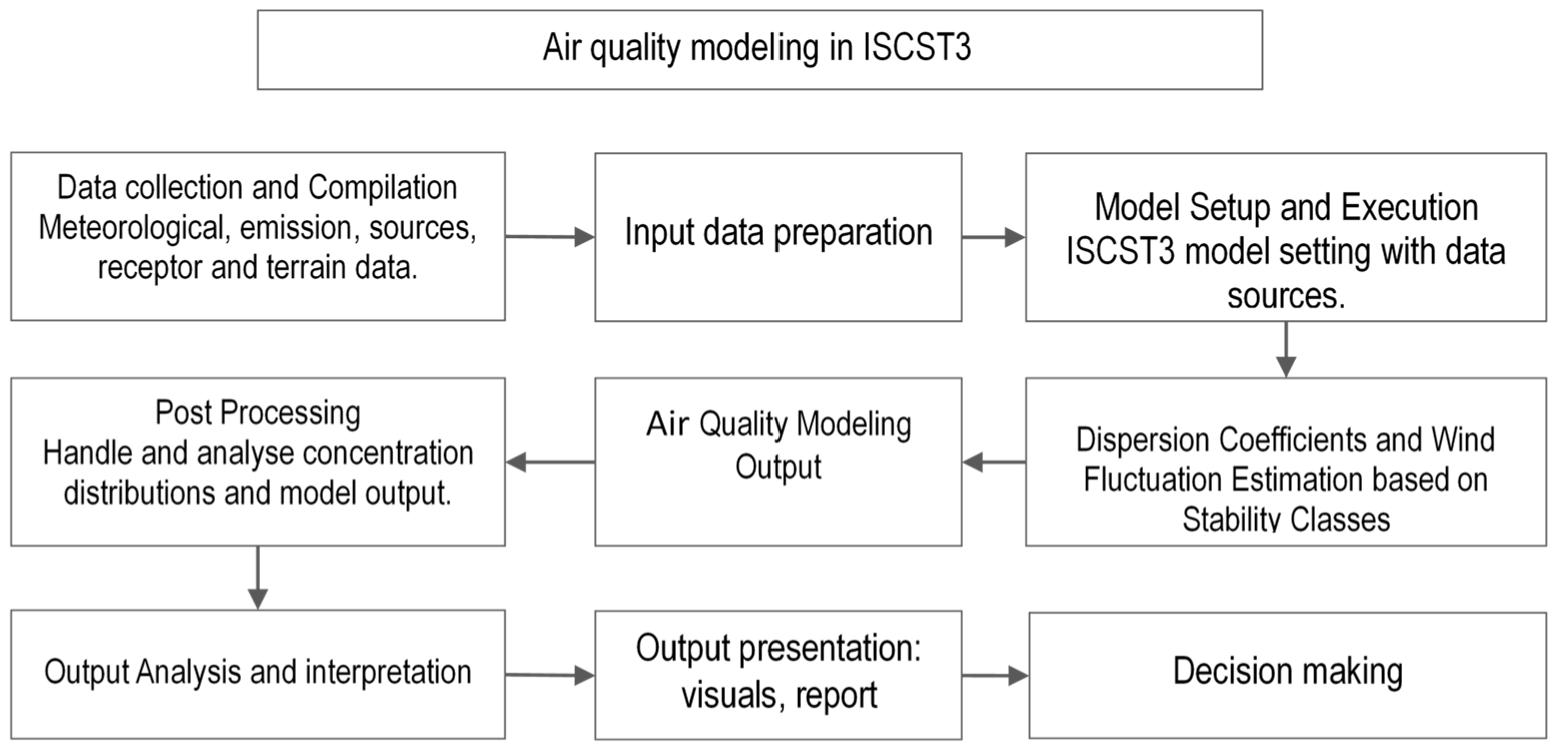
3.3.3. Air Quality Modeling
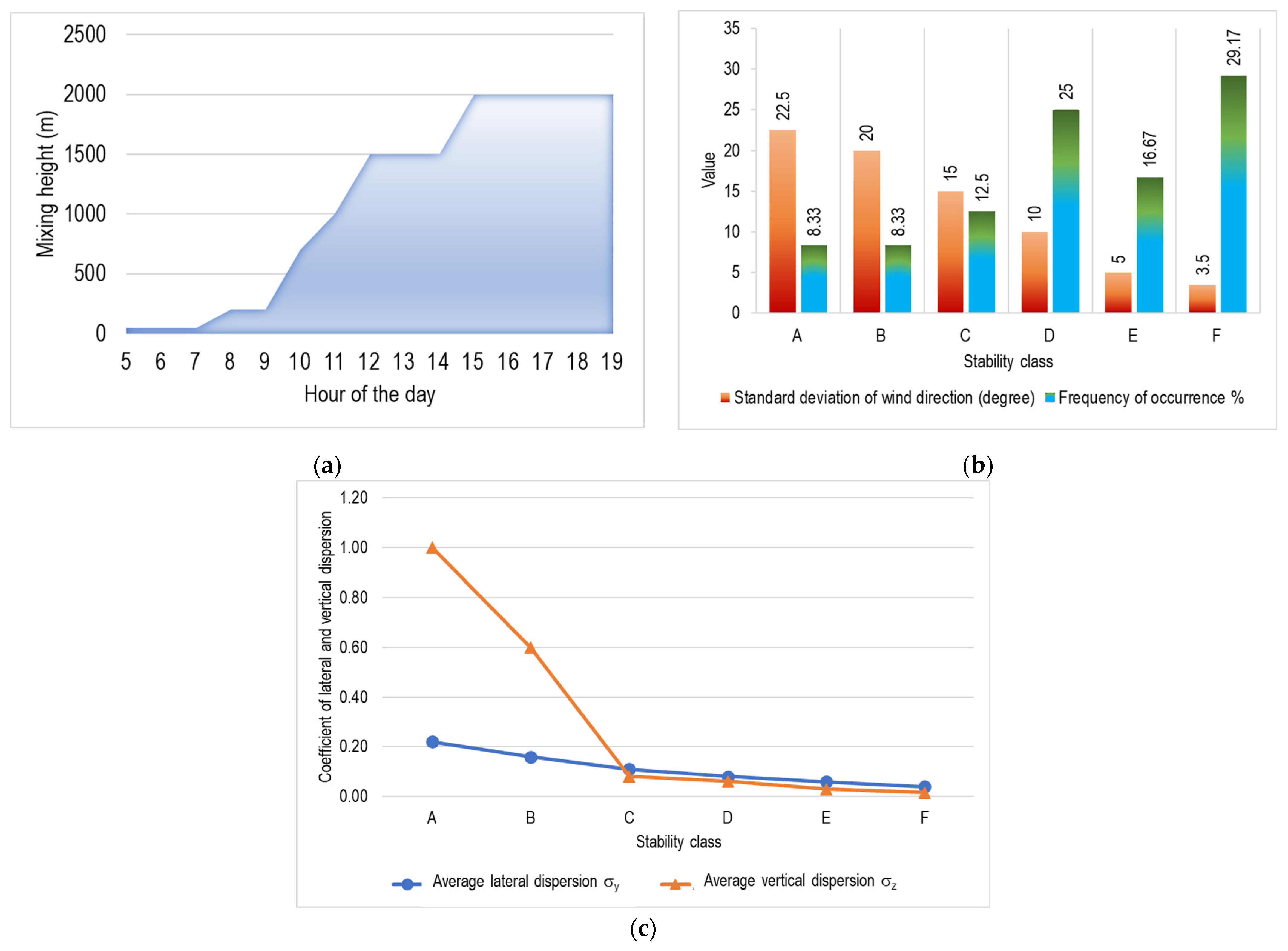
3.3.4. Stability Classification and Dispersion Parameters
3.3.5. Modeling Procedure
- Plume rise estimation: Briggs formulae, limited to the mixing layer.
- Buoyancy induced dispersion: Captures plume dispersion during ascent.
- Processing routine: Calms by default.
- Wind profile exponents: Default ‘Irwin’.
- Terrain: Flat terrain computation
- Transformation and removal: No physiochemical transformations or pollutant removal assumed.
- Washout by rain: Not considered.
4. Modeling, Analysis, and Results
4.1. Model Simulations and Analysis
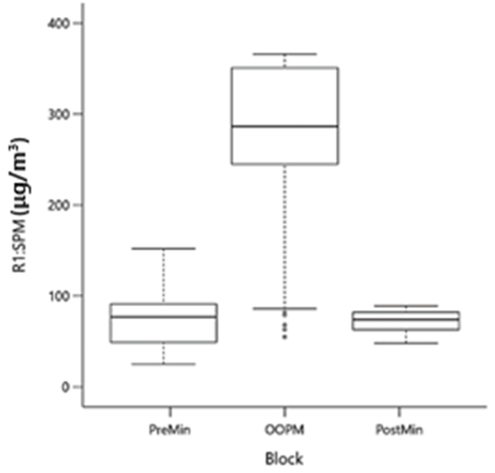
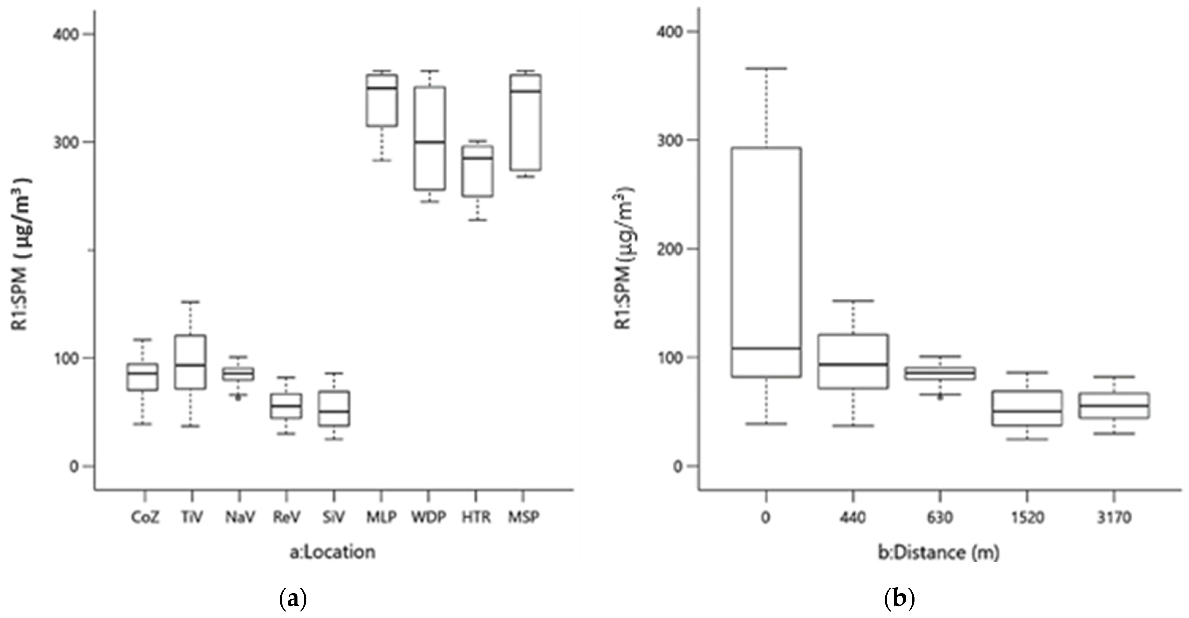
4.2. Exploratory Data Analysis
5. Conclusions
Supplementary Materials
Author Contributions
Funding
Institutional Review Board Statement
Informed Consent Statement
Data Availability Statement
Acknowledgments
Conflicts of Interest
References
- Mancini, L.; Nuss, P. Responsible Materials Management for a Resource-Efficient and Low-Carbon Society. Resources 2020, 9, 68. [Google Scholar] [CrossRef]
- Dehghani, H.; Bascompta, M.; Khajevandi, A.A.; Farnia, K.A. A Mimic Model Approach for Impact Assessment of Mining Activities on Sustainable Development Indicators. Sustainability 2023, 15, 2688. [Google Scholar] [CrossRef]
- Kampa, M.; Castanas, E. Human Health Effects of Air Pollution. Environ. Pollut. 2008, 151, 362–367. [Google Scholar] [CrossRef]
- Siddiqua, A.; Hahladakis, J.N.; Al-Attiya, W.A.K.A. An Overview of the Environmental Pollution and Health Effects Associated with Waste Landfilling and Open Dumping. Environ. Sci. Pollut. Res. 2022, 29, 58514–58536. [Google Scholar] [CrossRef] [PubMed]
- Skvarekova, E.; Tomaskova, M.; Zelenak, S.; Pacaiova, H. Analysis of Environmental Risk Factors in Selected Mining Activities. MM Sci. J. 2023, June, 6501–6506. [Google Scholar] [CrossRef]
- Park, S.; Song, D.; Park, S.; Choi, Y. Particulate Matter Generation in Daily Activities and Removal Effect by Ventilation Methods in Residential Building. Air Qual. Atmos. Health 2021, 14, 1665–1680. [Google Scholar] [CrossRef]
- Roy, S.K.; Nayak, D.; Rath, S.S. A Review on the Enrichment of Iron Values of Low-Grade Iron Ore Resources Using Reduction Roasting-Magnetic Separation. Powder Technol. 2020, 367, 796–808. [Google Scholar] [CrossRef]
- Ma, Y.; Wang, M.; Wang, S.; Wang, Y.; Feng, L.; Wu, K. Air Pollutant Emission Characteristics and HYSPLIT Model Analysis during Heating Period in Shenyang, China. Env. Monit. Assess. 2021, 193, 9. [Google Scholar] [CrossRef]
- Vig, N.; Ravindra, K.; Mor, S. Environmental Impacts of Indian Coal Thermal Power Plants and Associated Human Health Risk to the Nearby Residential Communities: A Potential Review. Chemosphere 2023, 341, 140103. [Google Scholar] [CrossRef] [PubMed]
- Gałaś, S.; Gałaś, A. The Qualification Process of Mining Projects in Environmental Impact Assessment: Criteria and Thresholds. Resour. Policy 2016, 49, 204–212. [Google Scholar] [CrossRef]
- Asif, Z.; Chen, Z.; Han, Y. Air Quality Modeling for Effective Environmental Management in the Mining Region. J. Air Waste Manag. Assoc. 2018, 68, 1001–1014. [Google Scholar] [CrossRef] [PubMed]
- Li, F. Documenting Accountability: Environmental Impact Assessment in a Peruvian Mining Project. PoLAR Political Leg. Anthropol. Rev. 2009, 32, 218–236. [Google Scholar] [CrossRef]
- Srivastava, A.; Kumar, A.; Elumalai, S.P. Evaluating Dispersion Modeling of Inhalable Particulates (PM10) Emissions in Complex Terrain of Coal Mines. Environ. Model. Assess. 2021, 26, 385–403. [Google Scholar] [CrossRef]
- Kumar, A.; Dixit, S.; Varadarajan, C.; Vijayan, A.; Masuraha, A. Evaluation of the AERMOD Dispersion Model as a Function of Atmospheric Stability for an Urban Area. Environ. Prog. 2006, 25, 141–151. [Google Scholar] [CrossRef]
- Gibson, M.D.; Kundu, S.; Satish, M. Dispersion Model Evaluation of PM2.5, NOx and SO2 from Point and Major Line Sources in Nova Scotia, Canada Using AERMOD Gaussian Plume Air Dispersion Model. Atmos. Pollut. Res. 2013, 4, 157–167. [Google Scholar] [CrossRef]
- Awuah-Offei, K.; Adekpedjou, A. Application of Life Cycle Assessment in the Mining Industry. Int. J. Life Cycle Assess. 2011, 16, 82–89. [Google Scholar] [CrossRef]
- Gupta, H.; Rao, B.P.; Pandit, V.I.; Hasan, M.Z. Air Pollution Modeling: A Tool for Management of Regional Air Quality. Indian. J. Env. Health 2002, 44, 1–7. [Google Scholar]
- Singh, K. Air Pollution Modeling. Int. J. Adv. Res. Ideas Innov. Technol. 2018, 4, 208–214. [Google Scholar]
- Ghose, M.K. Generation and Quantification of Hazardous Dusts from Coal Mining in the Indian Context. Environ. Monit. Assess. 2007, 130, 35–45. [Google Scholar] [CrossRef]
- Sairanen, M.; Rinne, M.; Selonen, O. A Review of Dust Emission Dispersions in Rock Aggregate and Natural Stone Quarries. Int. J. Min. Reclam. Environ. 2018, 32, 196–220. [Google Scholar] [CrossRef]
- Ambastha, S.K.; Haritash, A.K. Emission of Respirable Dust from Stone Quarrying, Potential Health Effects, and Its Management. Environ. Sci. Pollut. Res. 2022, 29, 6670–6677. [Google Scholar] [CrossRef]
- Holnicki, P.; Kałuszko, A.; Trapp, W. An Urban Scale Application and Validation of the CALPUFF Model. Atmos. Pollut. Res. 2016, 7, 393–402. [Google Scholar] [CrossRef]
- Rzeszutek, M. Parameterization and Evaluation of the CALMET/CALPUFF Model System in near-Field and Complex Terrain—Terrain Data, Grid Resolution and Terrain Adjustment Method. Sci. Total Environ. 2019, 689, 31–46. [Google Scholar] [CrossRef] [PubMed]
- Yerramilli, A.; Dodla, V.B.R.; Challa, V.S.; Myles, L.; Pendergrass, W.R.; Vogel, C.A.; Dasari, H.P.; Tuluri, F.; Baham, J.M.; Hughes, R.L.; et al. An Integrated WRF/HYSPLIT Modeling Approach for the Assessment of PM2.5 Source Regions over the Mississippi Gulf Coast Region. Air Qual. Atmos. Health 2012, 5, 401–412. [Google Scholar] [CrossRef] [PubMed]
- Binkowski, F.S.; Roselle, S.J. Models-3 Community Multiscale Air Quality (CMAQ) Model Aerosol Component 1. Model Description. J. Geophys. Res. Atmos. 2003, 108. [Google Scholar] [CrossRef]
- Duflo, E.; Greenstone, M.; Pande, R.; Ryan, N. The Value of Regulatory Discretion: Estimates From Environmental Inspections in India. Econometrica 2018, 86, 2123–2160. [Google Scholar] [CrossRef]
- Giosanu, D.; Marian, M.C.; Zaharia, A. The Influence of Meteorological and Topographical Parameters on the Dispersion of PM10 and Co Pollutants. Curr. Trends Nat. Sci. 2021, 10, 92–98. [Google Scholar] [CrossRef]
- Moore, S.J.; Egerton, T.; Merolli, M.; Lees, J.; La Scala, N.; Parry, S.M. Inconsistently Reporting Post-Licensure EPA Specifications in Different Clinical Professions Hampers Fidelity and Practice Translation: A Scoping Review. BMC Med. Educ. 2023, 23, 372. [Google Scholar] [CrossRef]
- Analena, B.B.; Yetkin, B.; Glenna, L.L. Assessing the Scientific Support for U. S. EPA pesticide regulatory policy governing active and inert ingredients. J. Environ. Stud. Sci. 2023, 13, 1. [Google Scholar] [CrossRef]
- Mok, K.M.; Miranda, A.I.; Leong, K.U.; Borrego, C. A Gaussian Puff Model with Optimal Interpolation for Air Pollution Modelling Assessment. Int. J. Environ. Pollut. 2008, 35, 111–137. [Google Scholar] [CrossRef]
- Bajoghli, M. Comparison of Application of AERMOD and ISCST3 Models for Simulating the Dispersion of Emitted Pollutant from the Stack of an Industrial Plant in Different Time Scales; Archives of Occupational Health: Yazd, Iran, 2019. [Google Scholar] [CrossRef]
- Biswas, D. Assessment of Impact to Air Environment: Guidelines for Conducting Air Quality Modelling; Central Pollution Control Board (CPCB): New Delhi, India, 1998; Volume 70, p. 42. [Google Scholar]
- Mabey, P.T.; Li, W.; Sundufu, A.J.; Lashari, A.H. Environmental Impacts: Local Perspectives of Selected Mining Edge Communities in Sierra Leone. Sustainability 2020, 12, 5525. [Google Scholar] [CrossRef]
- Attri, S.D. Atlas of Hourly Mixing Height and Assimilative Capacity of Atmosphere in India; India Meteorological Department: New Delhi, India, 2008.
- Nair, P.R.; Parameswaran, K.; Kumar, S.V.S.; Rajan, R. Continental Influence on the Spatial Distribution of Particulate Loading over the Indian Ocean during Winter Season. J. Atmos. Sol. Terr. Phys. 2004, 66, 27–38. [Google Scholar] [CrossRef]
- Nikiforov, I.; Rahman, Z. Numerical Method for Steady Ideal 2-D Flows of Finite Vorticity with Applications to Vertical-axis Wind Turbine Aerodynamics. Wind Energy 2022, 25, 1464–1484. [Google Scholar] [CrossRef]
- Mahrt, L. Bulk Formulation of Surface Fluxes Extended to Weak-wind Stable Conditions. Q. J. R. Meteorol. Soc. 2008, 134, 1–10. [Google Scholar] [CrossRef]
- Mohan, M. Analysis of Various Schemes for the Estimation of Atmospheric Stability Classification. Atmos Environ. 1998, 32, 3775–3781. [Google Scholar] [CrossRef]
- Leroy, C.; Maro, D.; Hébert, D.; Solier, L.; Rozet, M.; Le Cavelier, S.; Connan, O. A Study of the Atmospheric Dispersion of a High Release of Krypton-85 above a Complex Coastal Terrain, Comparison with the Predictions of Gaussian Models (Briggs, Doury, ADMS4). J. Environ. Radioact 2010, 101, 937–944. [Google Scholar] [CrossRef]
- Ebrahimi, M.; Jahangirian, A. New Analytical Formulations for Calculation of Dispersion Parameters of Gaussian Model Using Parallel CFD. Environ. Fluid Mech. 2013, 13, 125–144. [Google Scholar] [CrossRef]
- Turner, D.B. Atmospheric dispersion modeling, A Critical Review. J. Air Pollut Control Assoc. 1979, 29, 502–519. [Google Scholar] [CrossRef]
- Balentine, H.W. Air Quality Impact Analysis. In Air Quality Permitting; Routledge: London, UK, 2018; pp. 93–114. [Google Scholar]


| Lithology | Thickness (m) |
|---|---|
| Laterite | 10 to 20 |
| Phyllitic clay | 20 to 25 |
| Lumpy iron ore | 5 to 7 |
| Blue dust | 20 to 40 |
| Limonitic/manganiferous clay | 25 to 55 |
| Siliceous clays/quartzite | 30 to 60 |
| Schists | Unknown (base) |
| Sl. No. | Model Name | Advantages | Disadvantages | Citation |
|---|---|---|---|---|
| 1 | AERMOD | Regulatory applications, applicable to various source types, complex terrain | Complex, less suitable for short-term assessments | [14,15] |
| 2 | CALPUFF | Multi-layered model, long-term assessments, considers complex terrain, land-use changes | Not suitable for short-term assessments | [22] |
| 3 | HYSPLIT | Trajectory model, regional transport patterns, local dispersion modeling | Too complex, not suitable for short-term assessments | [23,24] |
| 4 | CMAQ | Comprehensive regional model, multiple pollutants, and complex atmospheric processes | Not suitable for short-term assessments | [25] |
| 5 | ISCST3 | The gaussian plume model approach, needs less input data, less complicated, versatility for short-term area source modeling, suitable for flat terrains | Flat-terrain assumption may not be fully representative. | [8] |
| Stability Class | Standard Deviation of Wind Direction Fluctuation in Degrees | Lateral Dispersion | Vertical Dispersion | Frequency of Occurrence (%) |
|---|---|---|---|---|
| A | >22.5 | 8.33 | ||
| B | 22.4–17.5 | 8.33 | ||
| C | 17.4–12.5 | 12.5 | ||
| D | 12.4–7.5 | 25 | ||
| E | 7.4–3.5 | 16.67 | ||
| F | <3.5 | 29.17 |
| Parameter | Excavation | Loading of the Ore—OB | Loading of the Ore—Core Zone |
|---|---|---|---|
| Ore production (million tons/year) | 0.5 | 0.5 | 0.5 |
| Total working days | 220 | 220 | 220 |
| Operational hours | 10 | 10 | 10 |
| Total operational hours | 2200 | 2200 | 2200 |
| Activity rate (t/h) | 227.27 | 227.27 | 227.27 |
| Uncontrolled emission rate (gm/t/h) | 0.0236 | 0.0236 | 0.0236 |
| Emission factor (gm/t) | 0.0236 | 0.0236 | 0.0236 |
| Influence area (m2) | 70,300 | 70,300 | 70,300 |
| Source emission rate in area (g/s/m2) | 9 × 10⁻⁸ | 2 × 10⁻⁸ | 9 × 10⁻⁸ |
| Control efficiency (%) | 90% | 90% | 90% |
| Controlled emissions (g/s/m2) | 9.3 × 10⁻⁹ | 2.1 × 10⁻⁸ | 2.1 × 10⁻⁸ |
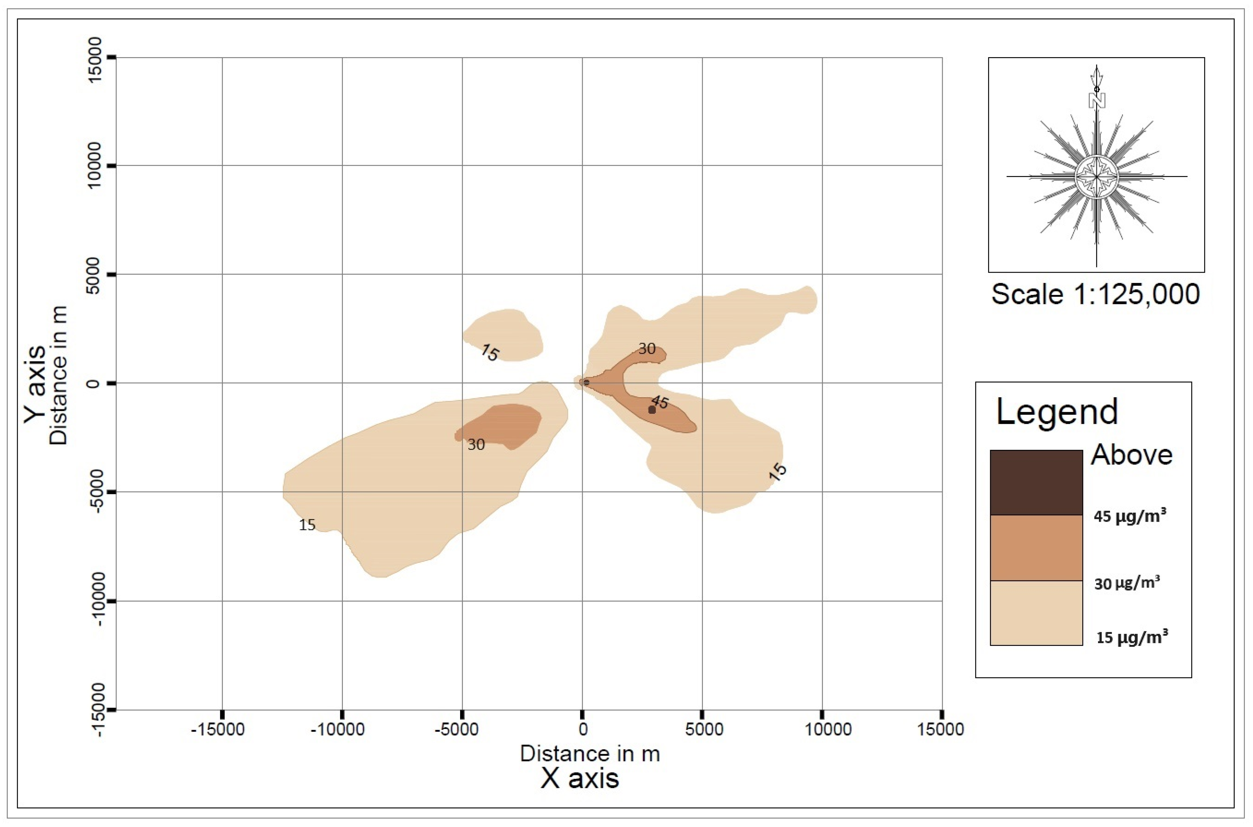
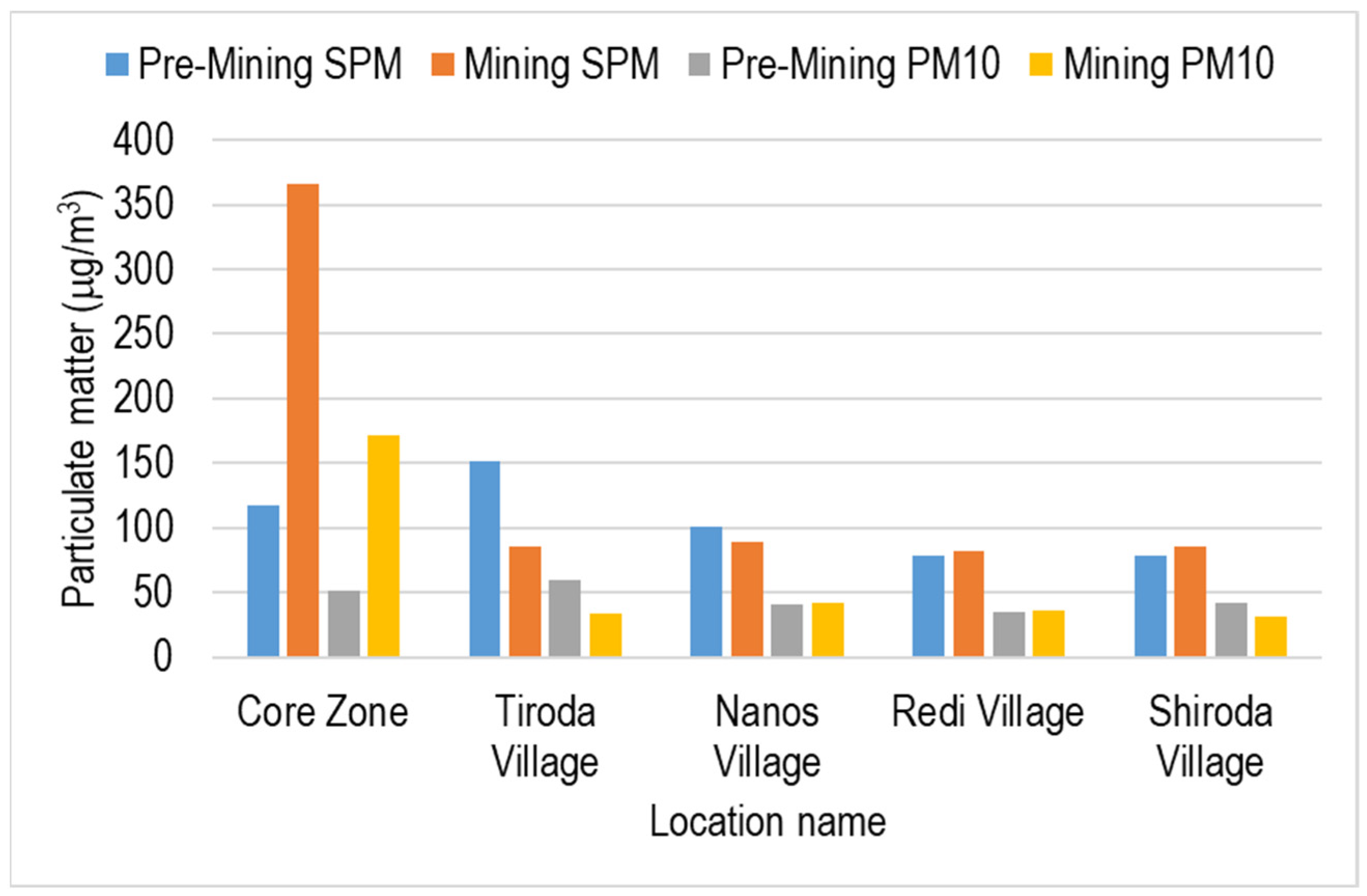
| Receptor Location | Cardinal Direction | Distance (m) | Baseline SPM (μg/m3) | Predicted Incremental SPM (μg/m3) | Estimated Total SPM (μg/m3) | Baseline PM10 + Predicted Incremental PM10 (μg/m3) |
|---|---|---|---|---|---|---|
| Core Zone | - | ~60 | 117 | 49 | 166 | 44.0 |
| Tiroda Village | N | 440 | 152 | 20 | 172 | 41.9 |
| Nanos Village | SE | 630 | 132 | 16 | 148 | 34.8 |
| Redi Village | SW | 3170 | 101 | 34 | 135 | 41.6 |
| Shiroda Village | NW | 1520 | 78 | 13 | 91 | 26.9 |
| Sl. No. | Mitigation Measure | Details | Advantages |
|---|---|---|---|
| 1 | Water-spray systems |
| Reduces airborne dust significantly and improves air quality for work persons and nearby communities. It also supports the plant growth and sustainability on-site |
| 2 | Stockpile management |
| Prevents the dust from being airborne, reduces overall environmental adverse impact, and enhances site cleanliness. |
| 3 | Vegetation buffer expansion |
| The vegetation buffer acts as a natural air filter, which also enhances the ecological aesthetics of the mining area and provides a habitat for local wildlife. |
| 4 | Administrative enhancements |
| Ensures compliance with environmental regulations and increases awareness and real-time air quality management |
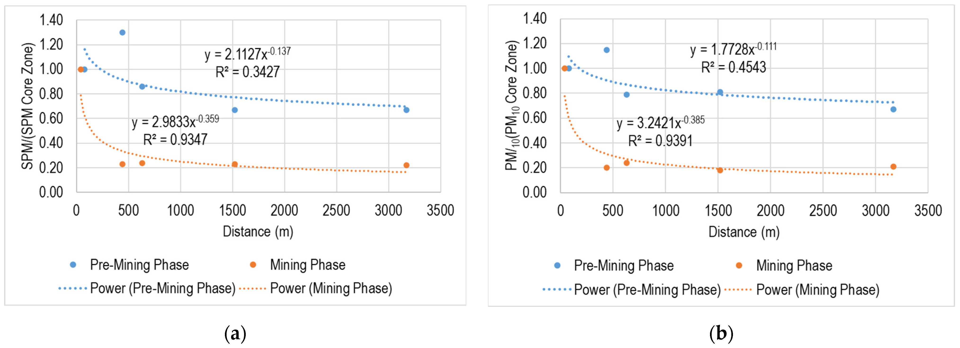
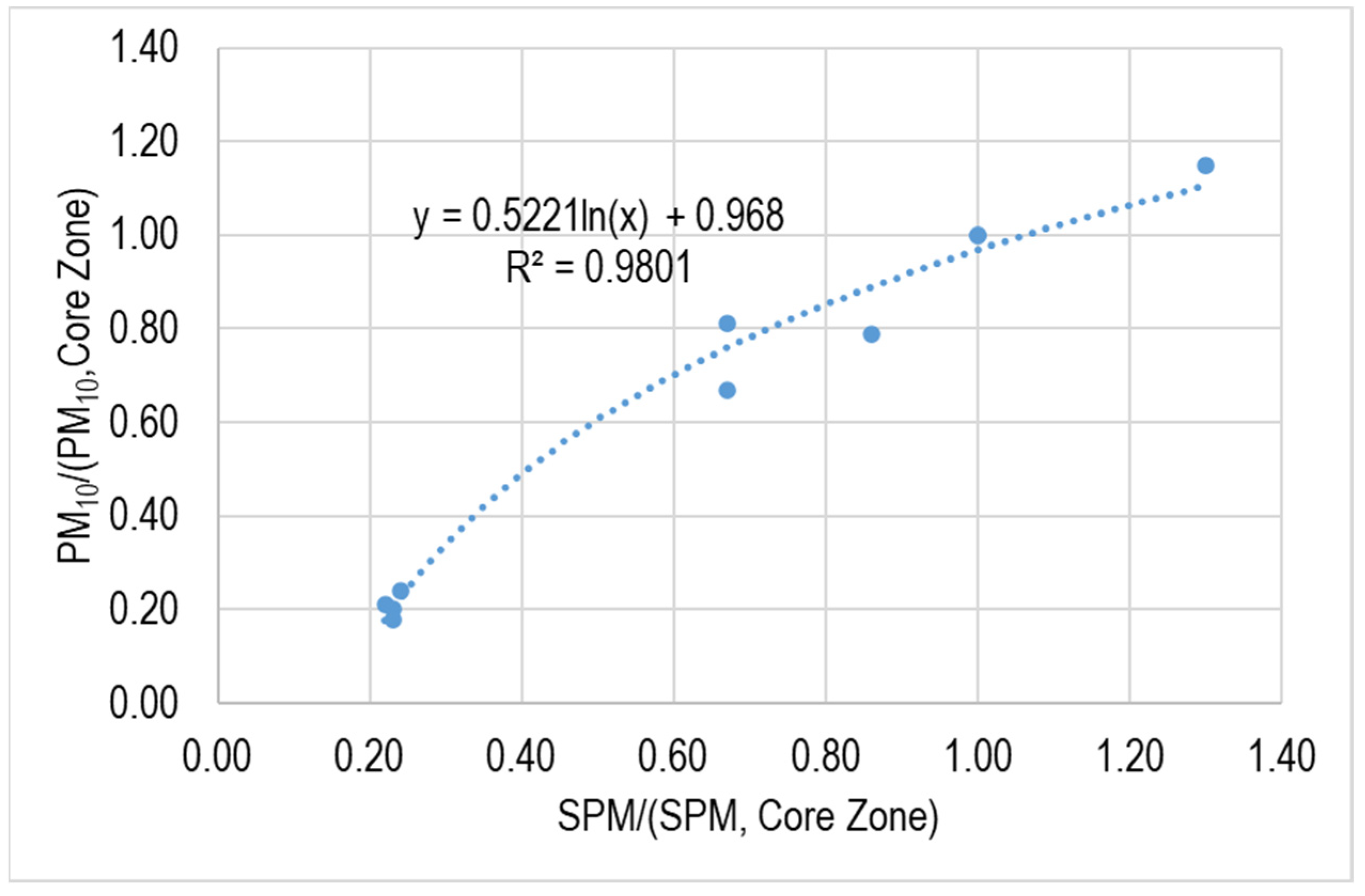
| Mining Phase | Location | Distance (m) | SPM to (SPM Core Zone) Ratio | PM10 to (PM10 Core Zone) Ratio | Change in SPM Mining Phase (%) | Remarks |
|---|---|---|---|---|---|---|
| Construction | Core Zone | ~60 | 1 | 1 | ||
| Construction | Tiroda Village | 440 | 1.3 | 1.15 | ||
| Construction | Nanos Village | 630 | 0.86 | 0.79 | ||
| Construction | Redi Village | 3170 | 0.67 | 0.67 | ||
| Construction | Shiroda Village | 1520 | 0.67 | 0.81 | ||
| Operation | Core Zone | 41 | 1 | 1 | 212.82 | |
| Operation | Tiroda Village | 440 | 0.23 | 0.2 | −43.42 | Mitigation measure used |
| Operation | Nanos Village | 630 | 0.24 | 0.24 | −11.88 | Mitigation measure used |
| Operation | Redi Village | 3170 | 0.22 | 0.21 | 5.13 | Increase 4 µg/m3 |
| Operation | Shiroda Village | 1520 | 0.23 | 0.18 | 10.26 | Increase by 8 µg/m3 |
Disclaimer/Publisher’s Note: The statements, opinions and data contained in all publications are solely those of the individual author(s) and contributor(s) and not of MDPI and/or the editor(s). MDPI and/or the editor(s) disclaim responsibility for any injury to people or property resulting from any ideas, methods, instructions or products referred to in the content. |
© 2024 by the authors. Licensee MDPI, Basel, Switzerland. This article is an open access article distributed under the terms and conditions of the Creative Commons Attribution (CC BY) license (https://creativecommons.org/licenses/by/4.0/).
Share and Cite
Katariya, N.K.; Choudhary, B.S.; Pandey, P. Air Quality Predictions through Mathematical Modeling for Iron Ore Mine Project. Appl. Sci. 2024, 14, 5922. https://doi.org/10.3390/app14135922
Katariya NK, Choudhary BS, Pandey P. Air Quality Predictions through Mathematical Modeling for Iron Ore Mine Project. Applied Sciences. 2024; 14(13):5922. https://doi.org/10.3390/app14135922
Chicago/Turabian StyleKatariya, Naresh Kumar, Bhanwar Singh Choudhary, and Prerna Pandey. 2024. "Air Quality Predictions through Mathematical Modeling for Iron Ore Mine Project" Applied Sciences 14, no. 13: 5922. https://doi.org/10.3390/app14135922