Roughness Evolution of Granite Flat Fracture Surfaces during Sliding Processes

Abstract

Roughness is an essential factor affecting the shear process of discontinuous surfaces, and the evolution of roughness is closely related to the mechanical behavior of discontinuous surfaces. In this paper, with the help of granite specimens, a direct shear test was carried out on flat fracture surfaces obtained by sawing in order to study the evolution of roughness with shear slip. During the tests, the roughness evolution was evaluated using the arithmetic mean, root mean square and power spectral density of the roughness. The variation in these parameters all indicate that the friction surface with large slip tends to be rougher, at least under the loading conditions in this paper. And the increase in normal force will enhance this process, while the loading rate seems to have little effect on the roughness evolution. Finally, the analysis of the power spectral density shows that the roughness evolution in the spatial frequency of the profile line is mainly reflected in the middle– and low–frequency part, while the high–frequency part corresponding to the microscopic roughness body does not change much throughout the shear process.

1. Introduction

Shear is a common mechanical process in nature, such as various friction processes in life, and landslides and earthquakes in the geology field are also related to shear [1,2]. There are many factors affecting the shear process, of which roughness is a more important one. During shear sliding, abrasive wear is constantly occurring and the geometry of the sliding surface, i.e., the roughness, is constantly changing, while the roughness also affects the sliding process in turn.

In a large number of shear–related studies, the morphology of the fracture surfaces before and after shearing is observed and recorded using electron microscopes [3,4] or scanners [5,6] in order to analyze the relationship between roughness and the shearing process. For example, Ji and Wu [6] recorded the morphology of granite fractures before and after fluid injection tests under triaxial conditions, and the results showed that after shearing, both saw–cut and natural fractures experienced roughness wear, and the natural fracture faces showed more wear. Meanwhile saw–cut fractures showed more seismic behavior. WangLei et al. [4,5] compared the morphology of sandstone fracture surfaces before and after triaxial tests and found the relationship between confining pressure and roughness from the analysis. In addition, materials such as casted specimens [7], salt rock [8] and homalite [9] have been employed in studies related to the roughness. Davidesko, Sagy [10] and Badt, Hatzor [11] studied the evolution of roughness with slip by conducting shear tests on rough fracture surfaces using limestone. And the most direct effect of roughness on the shear process is to change the shear strength and slip stability. Generally, the rougher the sliding surface, the higher the peak shear strength [12]. Specifically, however, attention is also paid to the strength of the material itself and the different failure modes [13,14,15,16] that occur during shear. Asperities with higher material strengths are less likely to be cut off and therefore produce higher shear strengths. Conversely, rougher bodies are sheared at lower strengths and are therefore relatively more stable, similar to the distinction between cut–off along the serration root and shear dilation that has been suggested in some studies [14,15,16]. Rough sliding surfaces also provide better stability [17], whereas smooth faults tend to produce larger stress drops, leading to larger earthquakes. In addition, it has been demonstrated that roughness has a significant effect on the pattern and length of seismic nucleation [18,19,20,21]. For smaller roughness, the roughness amplitude is significantly positively correlated with the length of nucleation. While for larger values of roughness amplitude, the discontinuity surface mainly exhibits aseismic slip.

The above studies give the correlation between roughness and strength, stability, and the effect of roughness on various behaviors in the friction process, which deeply reflects the important role played by roughness in the shear process. But the change rule of roughness itself is rarely studied. On the one hand, there exist a variety of indicators to measure roughness [22], and most of them are one sided. On the other hand, the change in friction surface morphology during shear is also random, and a large number of samples are needed to investigate the evolution process. However, the above laboratory tests usually only record the morphology of the fracture surface at the beginning and end of the test, and most of the tests were limited by the equipment, and the slip distances were only approximately ten millimeters, which resulted in very limited changes in roughness. Statistical data on a number of fault profiles by Sagy and Brodsky [23] show that the faults with small slips are rougher than those with large slips. In these results, field investigations of in situ faults, although more realistic, make it difficult to observe the evolution of roughness.

In this paper, through the shear test of granite flat fracture, combined with the three–dimensional scanner, the fracture surface after multiple, longer distance shear is measured, and the power spectral density and other multiple indicators are used to comprehensively analyze and summarize the evolution law of the roughness with slip in the shear process.

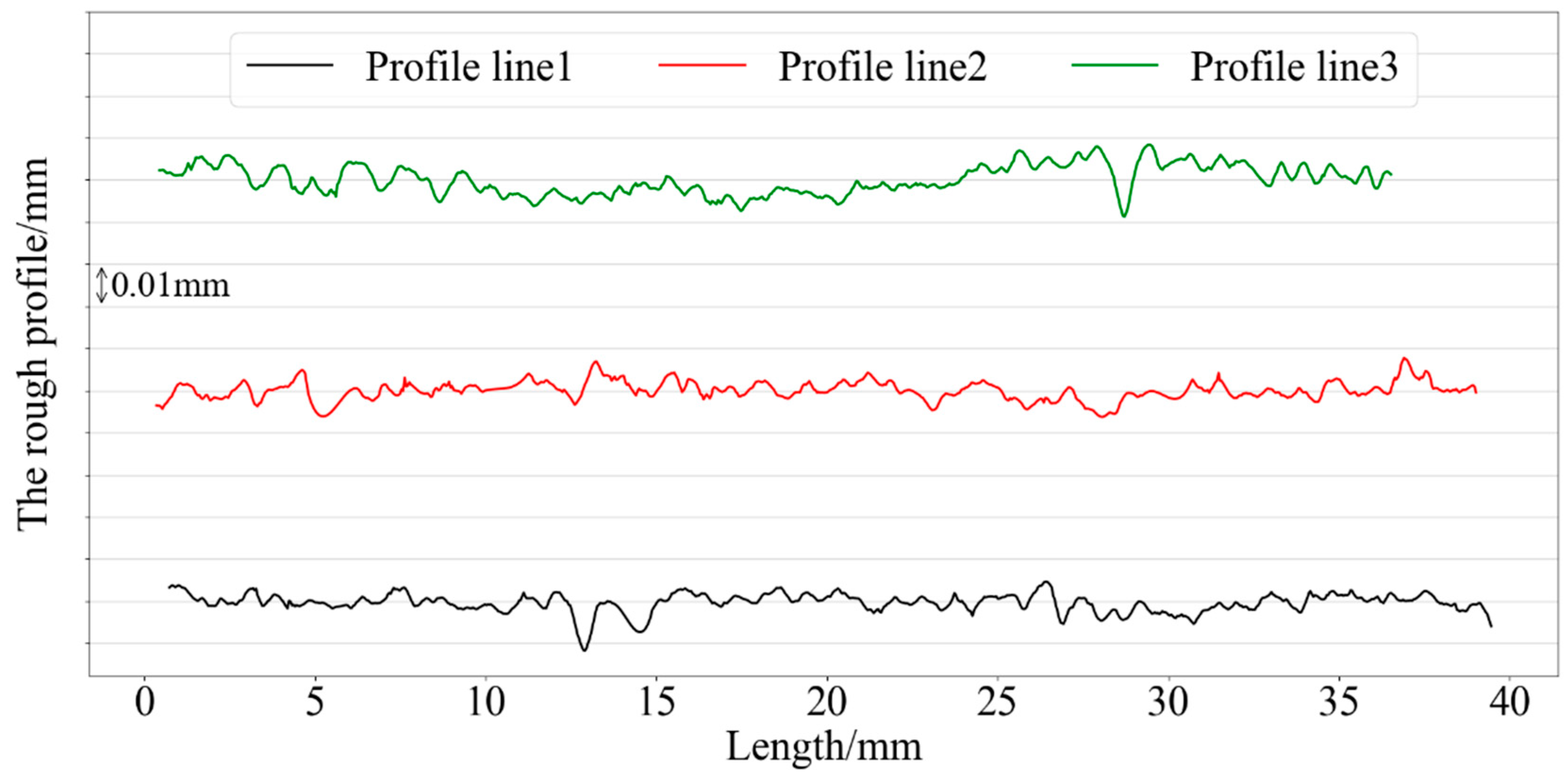
2. Roughness Measurement Indicators

Roughness is measured in a variety of indicators, which are usually categorized into three types [22]: amplitude parameter, spacing parameter, and hybrid parameter, of which amplitude parameter is the most common. The amplitude parameter is mainly based on the vertical coordinate value of the surface. For two–dimensional profile lines, there are the following types of amplitude parameters. The arithmetic mean deviation $Ra$ of the profile, defined as Equation (1), indicates the average of the absolute value of the vertical coordinate value $Z\left(x\right)$ within the sample length, which can most directly reflect the degree of the friction surface being worn out, and $l$ is the sample length of the profile line.

$$Ra=\frac{1}{l}{{\displaystyle \int }}_0^l\left|Z\left(x\right)\right|dx$$

(1)

The second amplitude parameter is, the root mean square (RMS) deviation of the profile, $Rq$, defined as in Equation (2), which represents the root mean square of the vertical coordinate, $Z\left(x\right)$, within the sample length, and reflects the extent to which the profile line deviates from the mean value.

$$Rq=\sqrt{\frac{1}{l}{{\displaystyle \int }}_0^{l}Z{\left(x\right)}^{2}dx}$$

(2)

The $Rsk$ skewness parameter is used to reflect the tendency of the assessed profile to be concave or convex; a negative value of $Rsk$ indicates that the profile lies more below the mean plane (valley), but since skewness is affected by a number of factors in the profile, it is discarded here.

In addition, JRC (joint roughness coefficient) proposed by Barton and Choubey [24] is also a common indicator of surface roughness. Many scholars have also carried out a large number of related studies around JRC, including those on the method of determining JRC [25,26], and those exploring the new, adapted to different conditions of the relationship between rock fracture surface shear strength and JRC [27,28]. However, JRC is controversial in its own quantification, is influenced by the subjective factors of the measurer. And when it is verified by back–calculation using the strength results obtained from the test, it tends to have a large discrepancy with the measurement results, and is currently only adapted to the 2D plane. Therefore, this indicator is not used in this paper for the time being.

In the above representation of roughness, the amplitude parameters such as $Ra$, $Rq$ only reflect the statistics of the longitudinal coordinate data of the rough surface, and miss the information of the horizontal direction of the rough profile. For example, for the two sinusoidal profiles shown in Figure 1, the amplitude is the same, but the curve frequency is different. If roughness indicators such as $Ra, Rq$ are used for calculation, the roughness obtained will be identical. Although there are also indicators that represent the spacing parameters in the horizontal direction, but they are all more one sided. Some recent studies [23,29,30,31] have shown that the roughness profile can be treated as a special signal, and the power spectral density obtained by discrete Fourier transform has a stable power–law relationship with the wavelength (or spatial frequency), such as Equations (3) and (4), or there is a linear relationship between the logarithms of the two, as written in Equations (5) and (6).

$$p=C\cdot {\mathsf{\lambda }}^{-\mathsf{\beta }}$$

(3)

$$p=C\cdot f^{\mathsf{\beta }}$$

(4)

$$\lg p=\lg C-\beta \lg \lambda$$

(5)

$$\lg p=\lg C+\beta \lg f$$

(6)

where $\lambda$ is the wavelength, $f$ is the spatial frequency, $f=1/\lambda$. $C$ and $\beta$ are constants. $p$ is the power spectral density (PSD), which is expressed as in Equation (7) for discrete data.

$$p_k={\left|FF{T}_{N,k}\left(Z\left(n\right)\right)\right|}^2={\left|{{\displaystyle \sum }}_{n=0}^{N-1}Z\left(n\right)e^{-\frac{j2\pi nk}{N}}\right|}^2$$

(7)

where $Z\left(n\right)$ is the data sequence of the rough profile for discrete sampling, $N$ is the number of all sampling points, $j$ is an imaginary unit, $n$ is the ordinal number of the discrete sampling points, and $k$ represents the number of cycles corresponding to a certain frequency within the sampling length in the frequency domain analysis, thus $0<k<N/2$ is required to ensure that there are at least two sampling points in each cycle. The power spectral density is the “signal” power in the unit frequency band (wavelength band) obtained by the Fourier transform on the roughness profile “signal”. That is to say, the irregular roughness profile is decomposed into several regular trigonometric curves, and Equation (3) (or Equation (4)) illustrates the relationship between the wavelength (or frequency) and amplitude of all the trigonometric curves. The advantage of the power spectral density (PSD) is that it embodies the evaluation effect of both the magnitude parameter through p and the spacing parameter through the included wavelength or frequency. It can be seen that PSD is a powerful tool to study roughness.

Next, the evolution law of the roughness during shear slip is analyzed in detail by carrying out shear tests on granite specimens with the help of the above indicators, $Ra, Rq, PSD$.

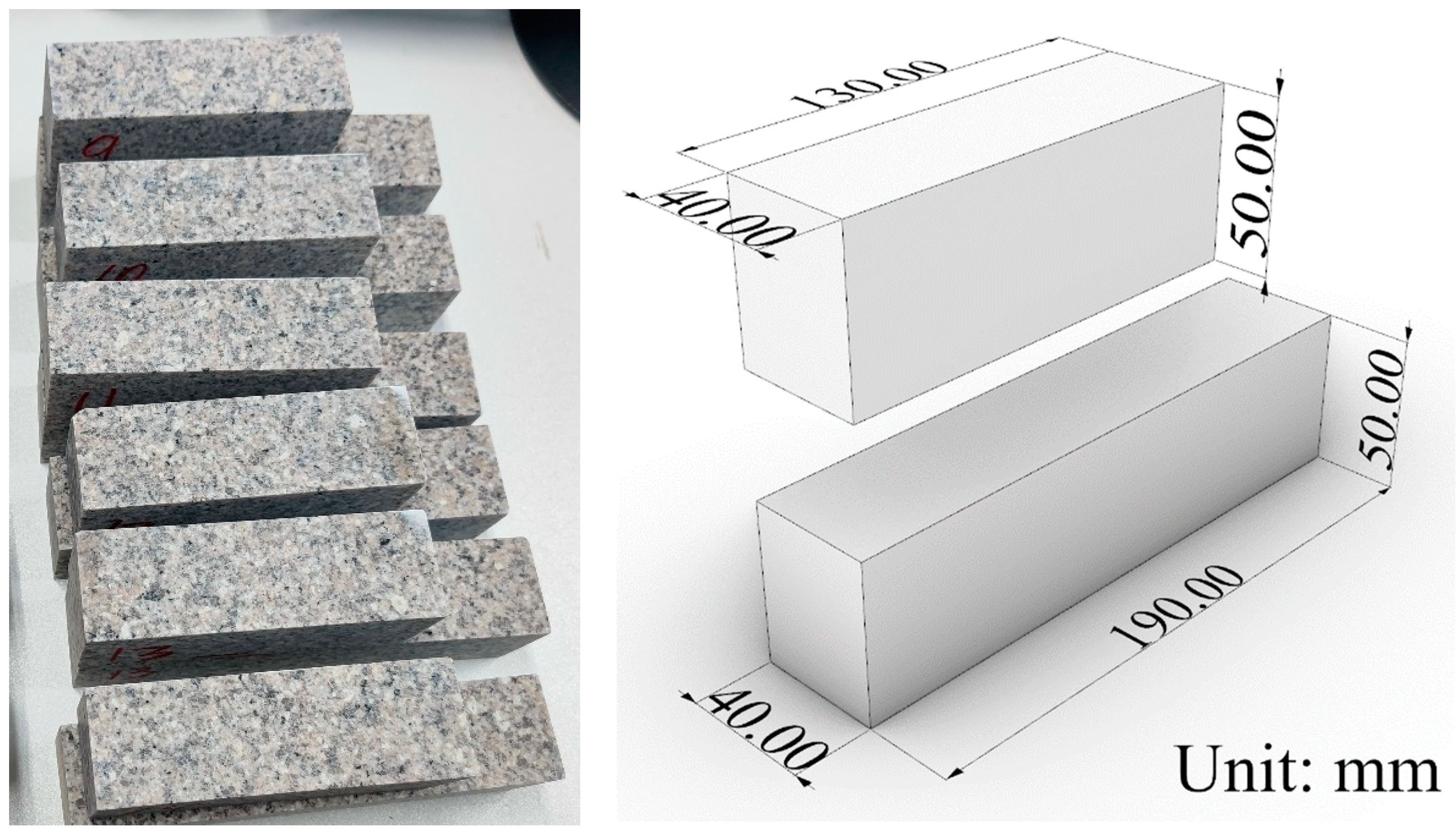
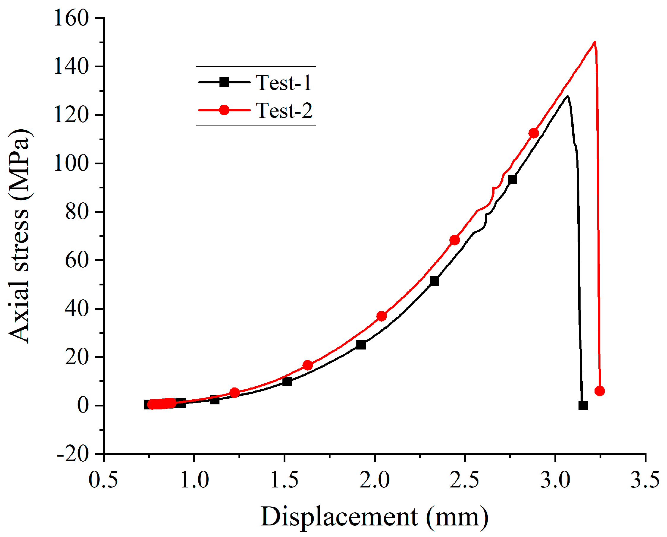
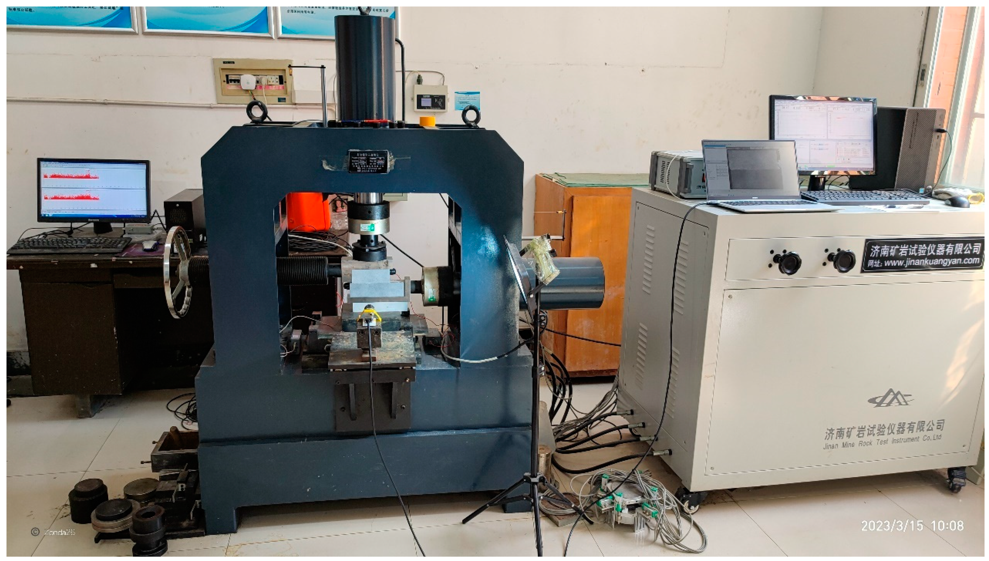
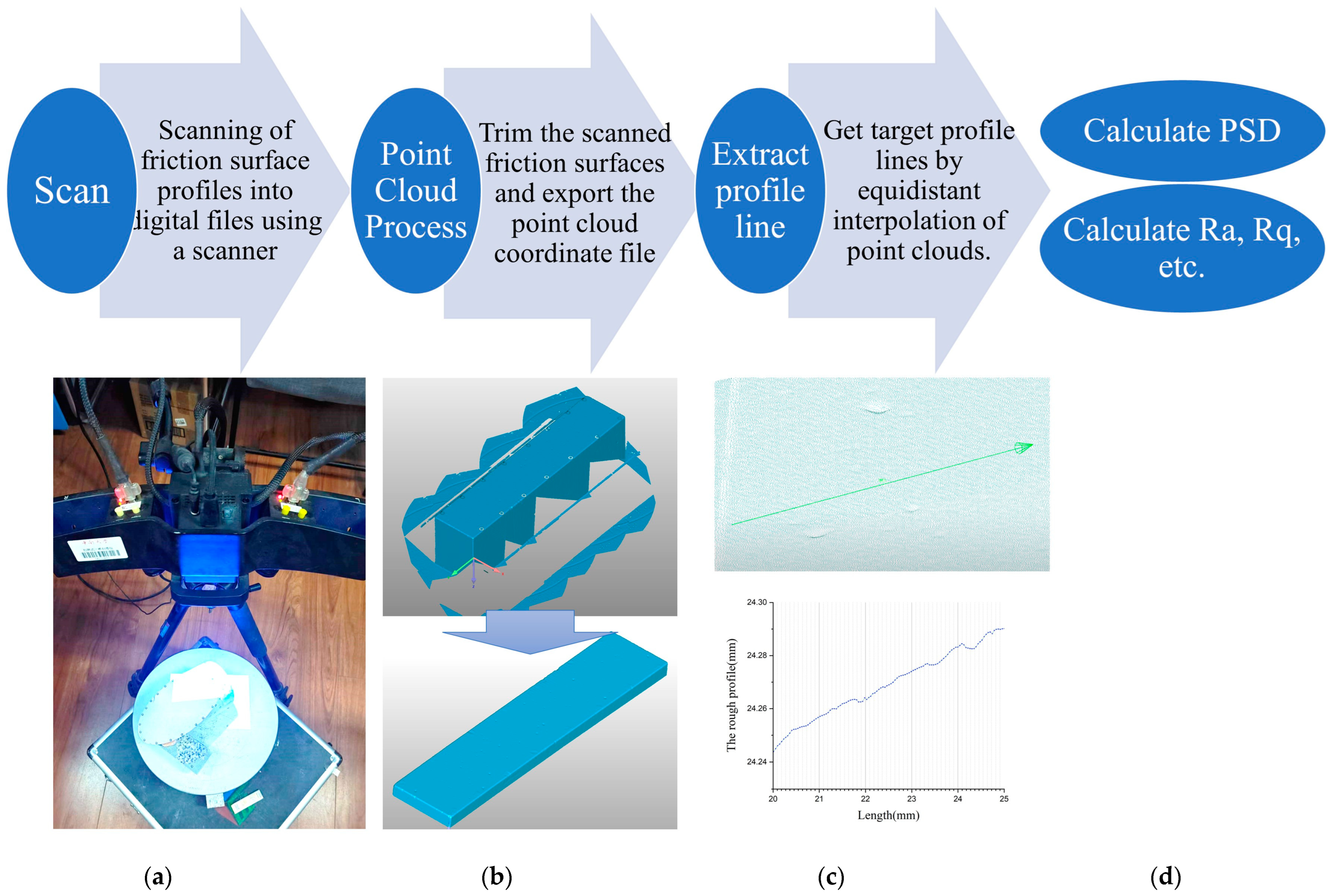
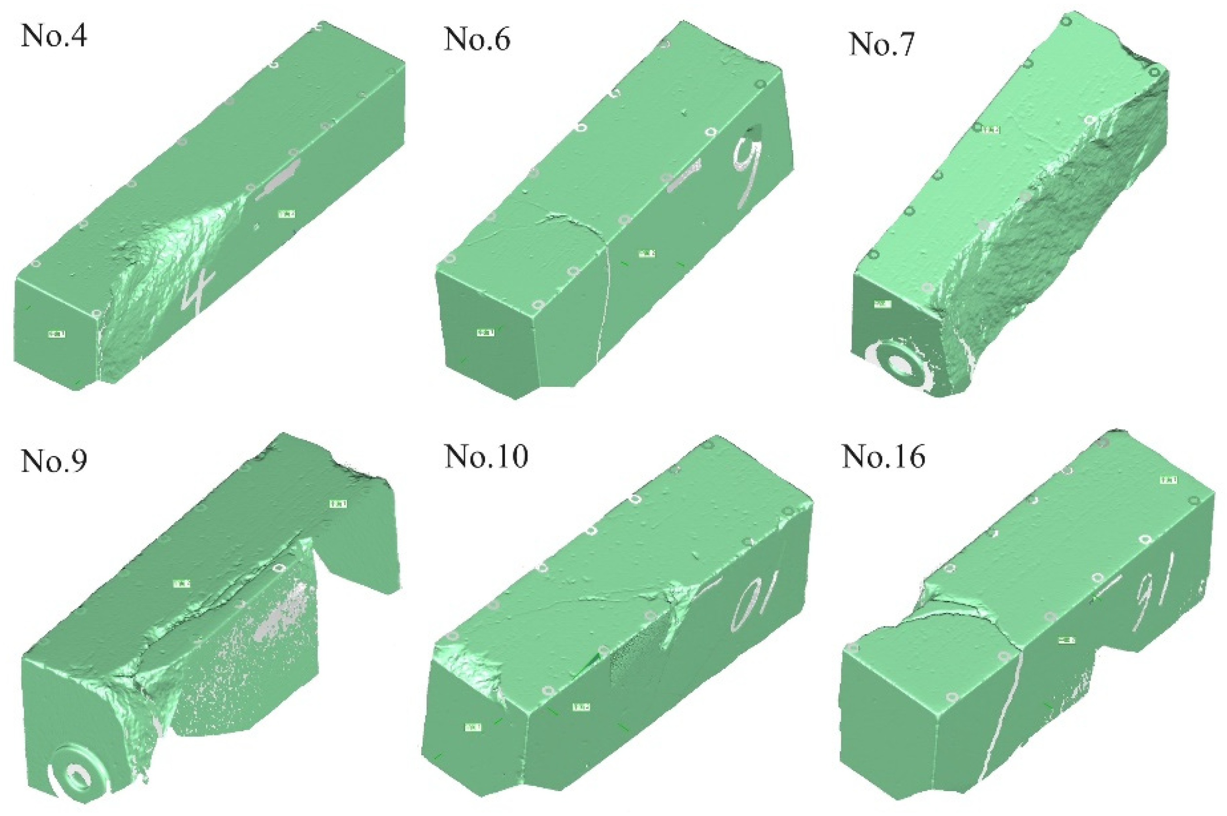
3. Experimental Preparation

Granite is one of the common rocks in nature, which is involved in many kinds of engineering projects such as enhanced geothermal system (EGS), and it is also often used to study the characteristics of rock masses in shear processes such as stick–slip and seismic nucleation. Therefore, in this paper, granite is chosen as the research object, and its dimensions are shown in Figure 2, the upper brick is 130 × 40 × 50 mm³, and the lower is 190 × 40 × 50 mm³. The uniaxial loading curve of this granite material is shown in Figure 3, and the uniaxial compressive strength is approximately 140 MPa, and the elastic modulus is approximately 10 GPa. In this paper, it is proposed to carry out the direct shear test on granite flat fracture, and the shear device is the YZW100 rock direct shear apparatus of Central South University, as shown in Figure 4, and acoustic emission monitors are used to monitor the shear process. The upper and lower parts of the specimen are not set to the same size due to the space limitation of the apparatus. For the current specimen size, a shear surface of 13 × 4 cm² can be allowed to slide 6 cm. In order to keep the initial state of the fracture surface consistent, all friction surfaces were obtained by sawing and polished, so that the initial flatness tolerance was controlled to within 10 μm. Some of the profiles are shown in Figure 5, where each scale of the longitudinal coordinates represents 0.01 mm.

A total of 4 sets of shears were performed on each pair of specimens throughout the test, with a shear distance of 80 mm per set (50 mm first, then the upper brick was placed back to its original position and reloaded by 30 mm). Due to the need for scanning, it was typically necessary to remove the fault gauge produced on the friction surface and clean and dry the surface following a set of shear loading. This process can be likened to a hydraulic fracturing operation performed on a granite mass in practice, in which the injection of fracturing fluid into a fracture causes a localized cleaning effect. In the analysis of how roughness evolves, two variables, namely normal force and loading rate, are set. These variables’ values are presented in

Table 1. Values of test variables.

Level	Normal Force $\mathit{\sigma }$/kN	Loading Rate $\mathit{v}$$/(\mathbf{mm}·{\mathbf{s}}^{-1}$)
Level 0	50	0.01
Level 1	100	0.05
Level 2	150	0.25

. The whole test contains 20 pairs of specimens, and the test variables corresponding to each pair of specimens are shown in

Table 2. Shear test program.

Specimen Number	2, 3, 9, 15	5, 11, 17	4, 7, 13, 14, 19, 20	6, 10, 16	8, 12, 18
Normal force level	$\sigma$−0	$\sigma$−1	$\sigma$−2	$\sigma$−1	$\sigma$−1
Loading rate level	$v$−1	$v$−1	$v$−1	$v$−0	$v$−2

.

Before loading the specimens with a direct shear apparatus, the initial topography of the friction surface was scanned once. The morphology of the friction surface was subsequently scanned every set of shear loading. The scanning device is the HOLON 3DX scanning system from HOLON Three-dimensional Technology (Shenzhen) Co., Ltd. in Shenzhen, China, employing a non-contact, photogrammetric 3D scanning method, as shown in Figure 6a, with a scanning accuracy of 0.01 mm.

As in Figure 6, the data processing procedure is presented. The specimen is first scanned as a point cloud using a photographic 3D scanner, and then the target surface is trimmed from it. Since the point cloud data are three–dimensional and irregularly distributed, the profile lines often do not pass through the data points when extracting the profile lines. Therefore, a 3D linear interpolation algorithm is employed to obtain equidistant distribution of profile line data based on the scanned point cloud. Firstly, all the points are projected onto the xy plane. Next, for a sample point of the profile line, the three nearest projected points are found, ensuring that the sample point is inside the triangle formed by these three projection points. Then, the vertical coordinate of the sample point is calculated by using Barycentric Interpolation. Finally, based on the above profile line data, the corresponding roughness indicator values are calculated according to Equations (1), (2) and (7).

Both friction surfaces in contact with each other were scanned during the test and 3 and 6 profile lines were taken in both directions parallel and perpendicular to the shear direction. In the later text, the profile lines parallel to the shear direction are denoted by V, while the perpendicular ones are marked by H. Additionally, the longer friction surface is noted as number 1 and the shorter one as 2.

4. Results

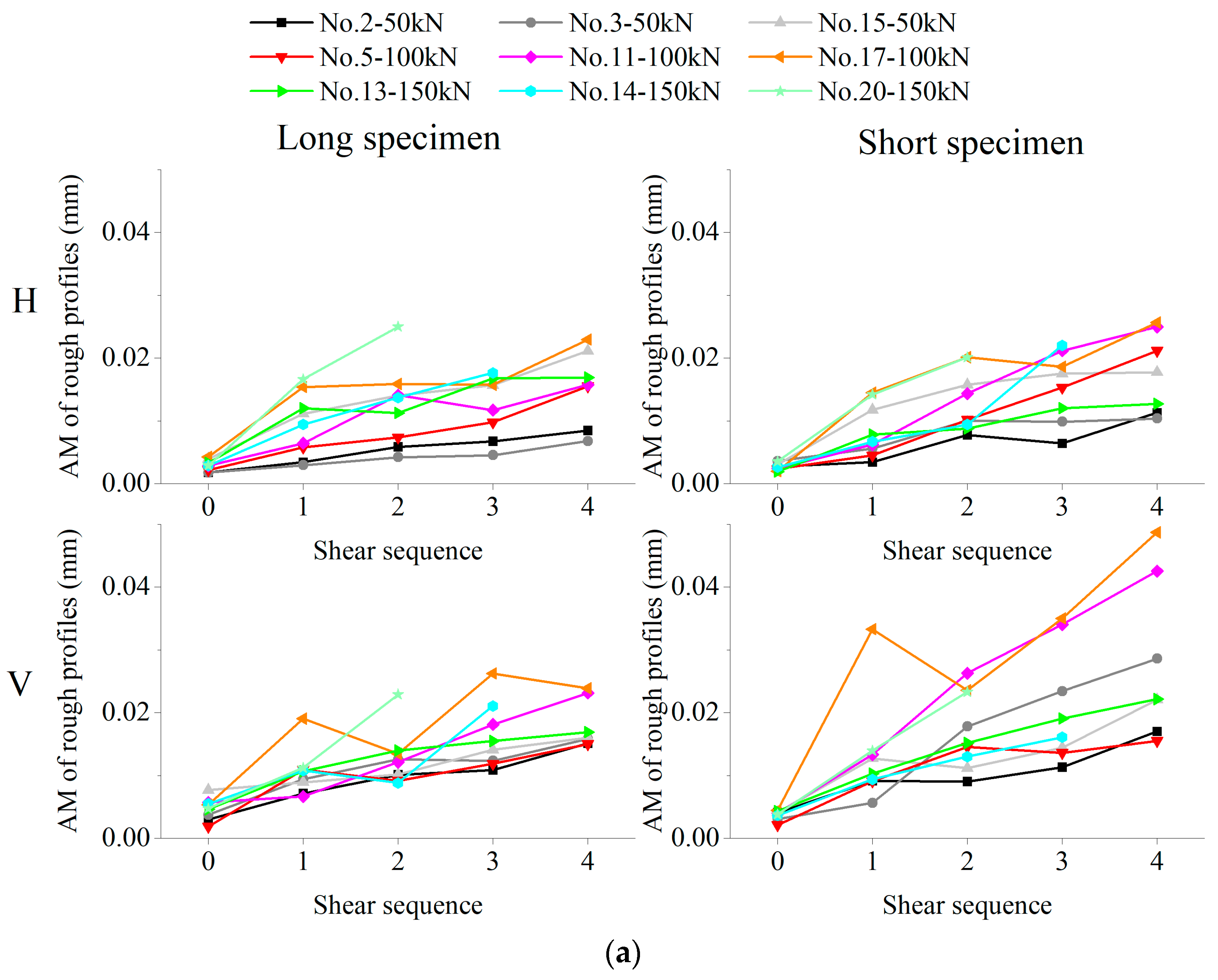
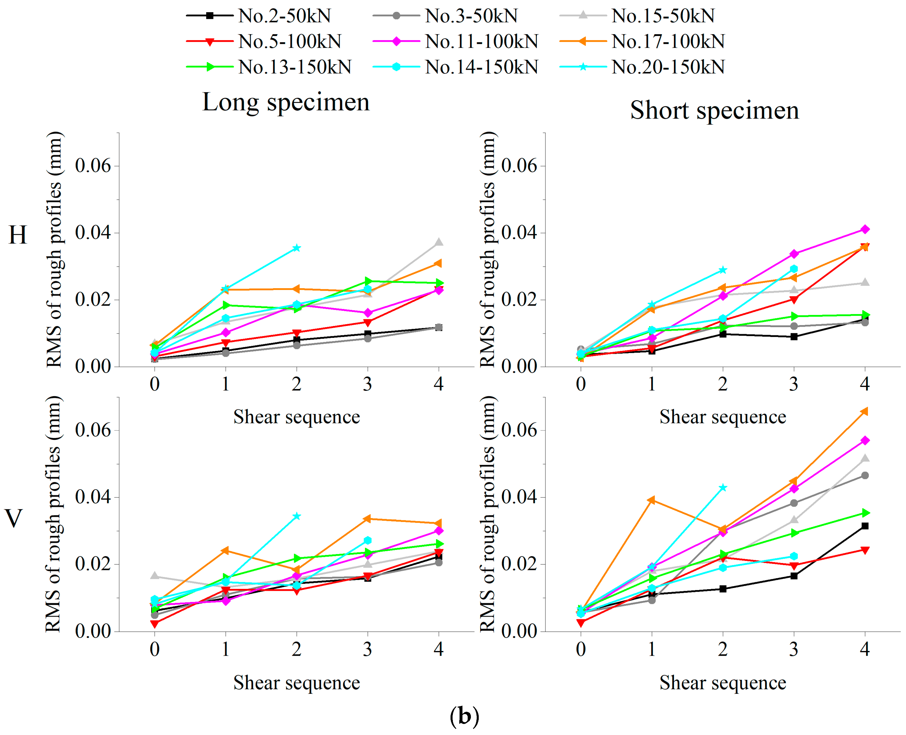
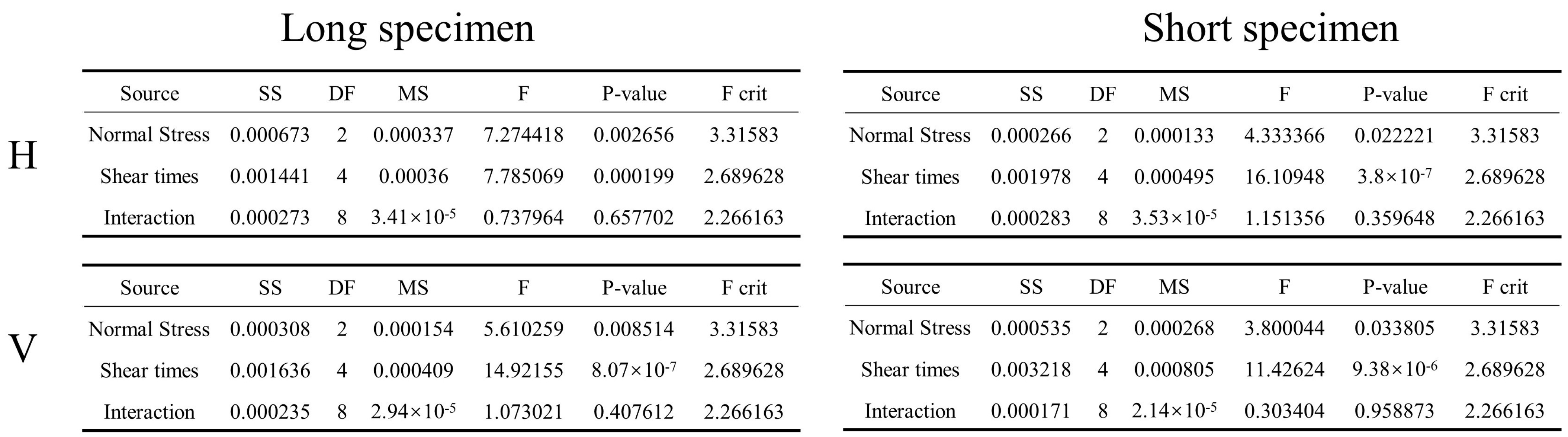
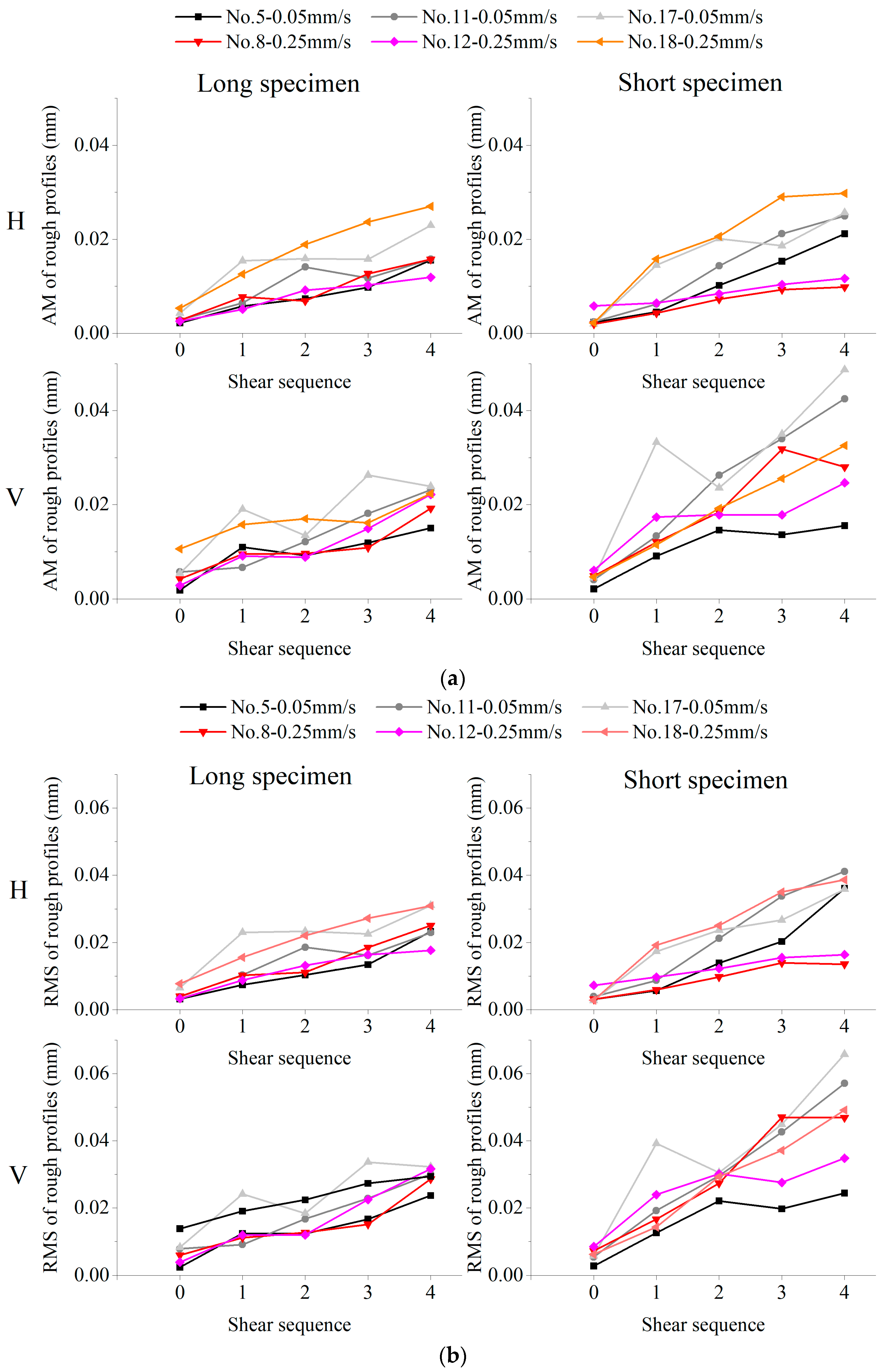
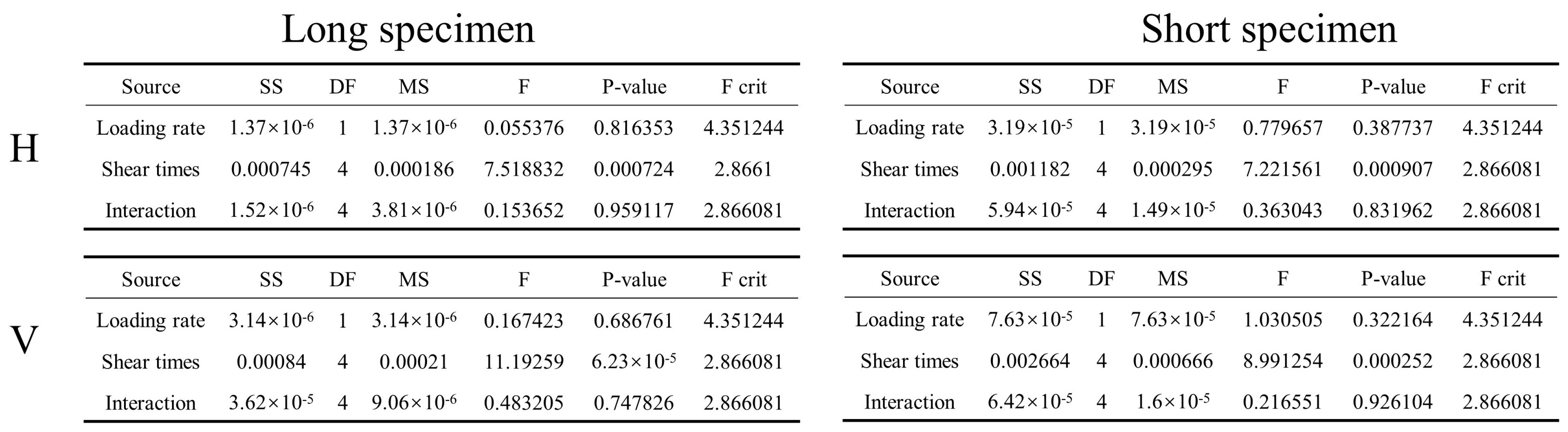
4.1. Summary of Amplitude Parameters

During the loading process, most of specimens that were under high normal force or low speed loading conditions experienced end shattering or side spalling at the first shear due to localized high stress at the end or side, as depicted in Figure 7. Therefore, these specimens were excluded from the roughness evolution analysis. The results of the remaining specimens were analyzed.

Since the position of both the scanner and the specimen cannot be kept absolutely fixed during scanning, the coordinate system of the friction surfaces from each scan is not consistent. Therefore, prior to calculating the amplitude parameters, the coordinate systems of all point clouds need to be unified. Then, a baseline of the profile line extracted from the unsheared specimen is calculated. This baseline is utilized as a reference to obtain the baseline of the profile lines in each scan of this specimen by fitting. Subsequently, these baselines are subtracted to derive the amount of wear on the friction surface of the specimen for each scan. The value of the desired magnitude parameter is calculated from Equations (1) and (2) finally. For each specimen, the roughness parameter value following each shearing operation is derived through the averaging of computational values obtained from multiple profile lines. And prior to calculating the mean, outliers are eliminated using the whisker range of the box plot to ensure the reliability of the data. For samples numbered 14 and 20, where the shear time is less than four, extrapolation methods are employed to supplement the partial data.

As shown in Figure 8, the two plots show the results of the two variables, arithmetic mean value and root mean square of the roughness profile line for various normal force conditions (No. 2 represents specimen numbered 2). The data for each variable are further differentiated between the upper and lower specimens and different directions. Overall, the arithmetic mean and the root mean square of the roughness profile tend to increase as the shear slip increases. These phenomena indicate that the roughness profile is being continuously abraded and the morphology of the whole profile is continuously downward concave; on top of that, the continuous shearing also makes the complexity of the profile line increasing. Due to the inconsistency of the specimen lengths, the short specimens are always in friction. As can be seen from the comparison in the graphs, the mean and RMS values of the shorter specimens are generally larger, which further suggests that the slip results in the roughness of the flat fracture surfaces to become larger. Moreover, this phenomenon seems to have a certain correlation with normal force, particularly in the H direction. The greater the normal force, the more significant the changes in $Ra$ and $Rq$. Next, taking the arithmetic mean as an example, a two-way repeated measures analysis of variance (ANOVA) is conducted. Here, the two factors refer to normal force and shear times. Prior to that, a normality test is performed on the data to ensure that the observed variables satisfy (approximately) the normal distribution, and a test of homogeneity of variances is also conducted. Finally, the ANOVA is completed in the “Data Analysis” module of Excel, and the results are presented in Figure 9, corresponding to the data in Figure 8a. As can be seen from Figure 9, regardless of the direction, the p-values corresponding to normal force and shear times are both less than 0.05. Therefore, it can be concluded that at a significance level of 0.05, normal force and shear times both have significant effects on roughness. Additionally, a comparison of the p-values indicates that the effect of shear times on roughness is more pronounced compared to normal force, and the interaction between the two factors does not have statistical significance.

Figure 10 is similar to Figure 8, the difference is that the control variable is the loading rate instead of the normal force. The rule of different variables with respect to the number of shears does not change, but the effect of loading rate is almost not observed from the figure. Similarly, conducting an analysis of variance (ANOVA) on the data in Figure 10a, the results are presented in Figure 11. It can be observed that the p-value corresponding to the loading rate is consistently greater than 0.05, indicating that the loading rate does not have a significant impact on roughness.

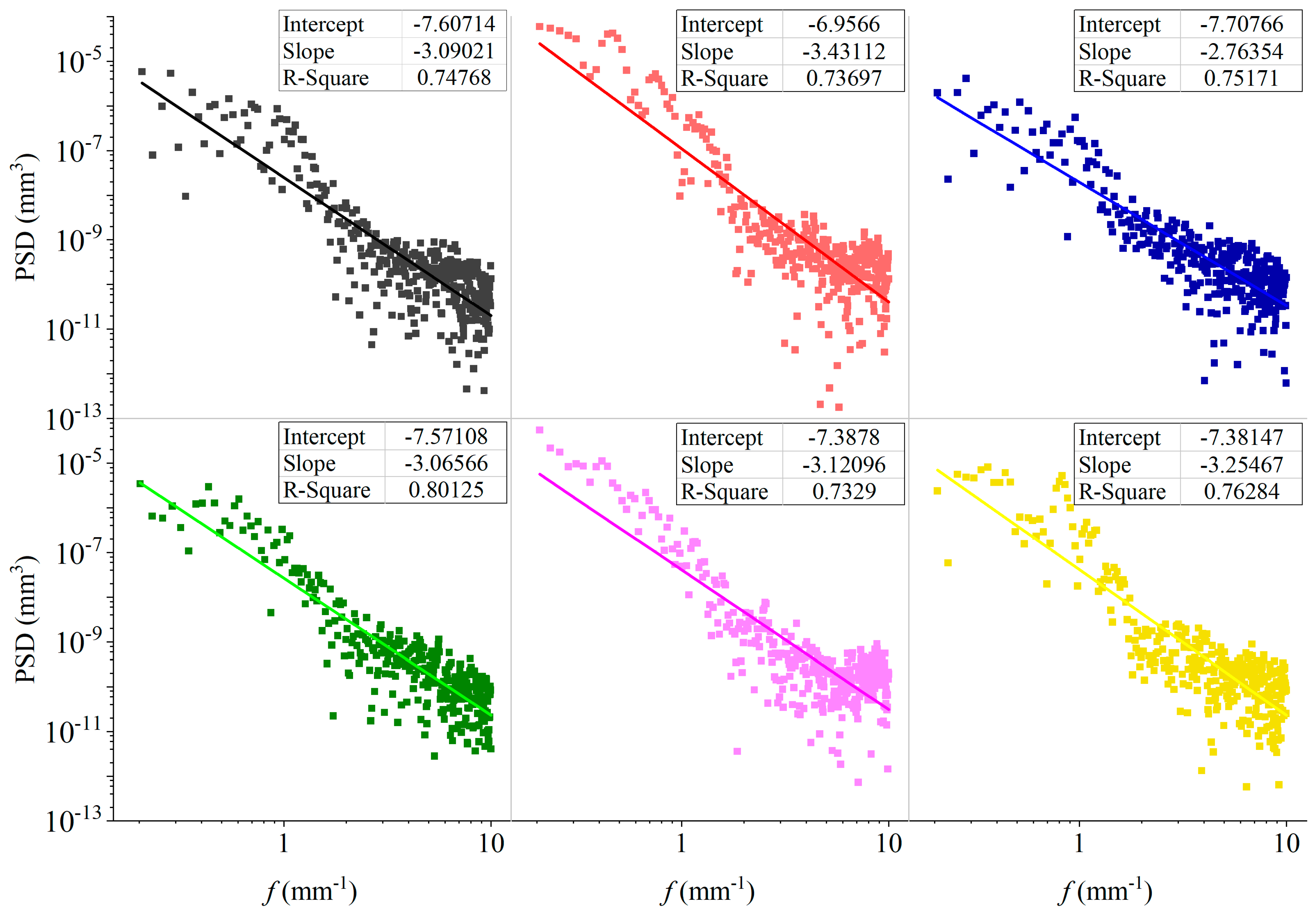
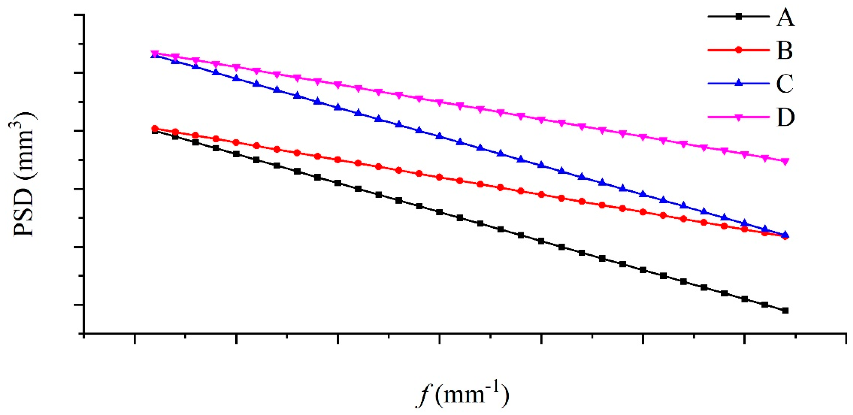
4.2. Summary of Power Spectral Density with Shear Slip

The fast Fourier transform (FFT) was applied to all the profile lines and the corresponding PSD–f frequency–spectral relationships were calculated. During the FFT calculation, a Hanning window was introduced to reduce data leakage. And for the H–direction profile lines, the data were analyzed by taking the spatial frequency interval of 0.2~10 ${\mathrm{mm}}^{-1}$, which corresponds to the wavelength range of 0.1~5 mm; Meanwhile, the V–direction profile line data were evaluated using a spatial frequency interval of 0.0166~10 ${\mathrm{mm}}^{-1}$, which corresponds to a wavelength range of 0.1~60 mm. Taking Figure 12 as an example, it can be seen that there is a linear relationship between the logarithms of both the PSD and the spatial frequency f. This means that the low–frequency part of the curve typically correspond to larger amplitudes, while the high–frequency part tends to have small amplitudes. The low–frequency and high–frequency parts correspond to waviness and roughness, respectively, as described in some published works [32,33,34,35]. The linear fit then gives the slope and intercept, which are the parameters β, lgC in Equation (7).

Next, the results of the specimen with a normal force of 50 kN and a loading speed of 0.05 mm/s are taken as an example to analyze the changes in the above fitting parameters, as shown in Figure 13. The scatter points in the graph represent the values of the fitting parameters obtained from the processing of a single profile line after each shear. The average values of the fitted parameters for all profile lines per shear were then calculated and plotted as dotted lines. In each subplot, the x-axis indicates the shear sequence, while the left graph shows the results for the friction surface of the longer specimen in the lower part and the right one shows the results for the shorter specimen in the upper part.

Overall, as the number of shears increases, the intercept $\lg C$ obtained from the fitting continuously increases in both directions, and the intercept value perpendicular to the shear direction is significantly larger than that parallel to the shear direction. This can be easily understood by the fact that as the shear slip increases, the notch on the friction surface becomes deeper and deeper, i.e., the amplitude of the rough surface profile line becomes larger and larger, thus leading to a gradual increase in the intercept $\lg C$. Since each shear is the same, it can be assumed that the intercept $\lg C$ increases approximately linearly with the shear distance, which means that each shear results in an exponential increase in the amplitude increment. The notches formed by shearing are mainly parallel to the shear direction, thus leading to larger fitting parameters for profile lines perpendicular to the shear direction. At the same time the morphology of the friction surface parallel to the shear direction is changing.

For the slope $\beta$, different patterns are exhibited in the two directions. Perpendicular to the shear direction, the value of the slope obtained from the fitting shows a significant decreasing trend with the shear distance, while parallel to the shear direction, it shows less variation, except that the fitted slope of the friction surface of the upper part slightly decreases. Since the slope is negative in the PSD–f relationship, it also indicates that the rough surface profile perpendicular to the shear direction has an increasing amplitude in the low–frequency part with the increasing number of shears. In comparison, the overall spectral distribution of the rough surface profile profile parallel to the shear direction remain relatively stable, but the amplitude is getting larger.

Figure 14 briefly illustrates the effect of slope and intercept on the PSD–f relationship, with larger slopes in B and D, and larger intercepts in C and D. During shearing, most of the specimens show an increase in the intercept and a decrease in the slope. This can be regarded as a shift of the PSD–f relationship of the roughness profile from B to C in Figure 14, which means that the roughness parts, which are mainly low–frequency and with wavelengths on the order of mm, are heavily changed. Regarding the criteria for the division of the frequency bands, it can be simply seen from Figure 12 that 1 ${\mathrm{mm}}^{-1}$ can be roughly used as the dividing line between high and low frequencies. In order to distinguish the two frequency bands more clearly, in the roughness profile line analysis perpendicular to the shear direction, the part smaller than 1 ${\mathrm{mm}}^{-1}$ is defined as low frequency, the part larger than 2 ${\mathrm{mm}}^{-1}$ as high frequency, and the middle part as medium frequency. Parallel to the shear direction, 0.75 and 2 ${\mathrm{mm}}^{-1}$ were used as the cut–off points for the three frequency bands. The variation in the fitted parameters in the three frequency bands for all the profile lines is analyzed in detail below, and the data in the different bands similar to those in Figure 13 are summarized in Figure 15.

As can be seen in Figure 15, there is a clear difference between the trends of the fitted parameters corresponding to the different frequency bands. For the H direction perpendicular to the shear direction, the intercept in the high–frequency part does not change much, and the slope increases slightly but not significantly; while for the mid–frequency and the low–frequency part, most of the specimens show a significant increase in the intercept in both directions, while the slope decreases significantly. This clearly verifies the previous hypothesis that the changes in roughness during shearing are mainly concentrated in the relatively low–frequency part, which corresponds to the part with a spatial wavelength greater than 0.5 mm. That is to say, under the size of the specimens and the test conditions in this paper, in the direction perpendicular to the shear direction, the friction mainly creates “notches” with a width greater than 0.5 mm, which is the largest change in the whole profile. Smaller–scale asperity and microscopic contact did not change much during shearing. The amplitude of the roughness profile continued to increase over the limited number of shears (4) and shear distances (~320 mm) in this test, and showed no signs of weakening or stabilization.

In the V direction, the evolution laws of slope and intercept in the three frequency bands keep basically the same trend as in the H direction. However, there are some differences in the specific values, the intercept in the H direction is generally larger than that in the V direction by 0.5 to 1, which means that the roughness amplitude produced in the V direction is nearly an order of magnitude smaller than that in the H direction. And in terms of slope, the V direction is generally larger. Therefore, the change rule in the fitting parameters in the V direction indicates that, besides the obvious notches produced in the H direction, in the direction parallel to the shear direction, the roughness is also undergoing the same change, and some similar “dents” also appear in the sliding surface, although not visible relative to the naked eye.

5. Discussion

Previous studies [10,23,29] have found that for shearing of rough fracture surfaces generated from a splitting test, the fracture surfaces become increasingly smoother as the shear displacement increases. Scholars have also conducted statistical analysis on natural fault surfaces and have concluded that large slip faults tend to be smoother. In the present experiment, as in Figure 5, the initial state of the fracture surface is “smooth”. Variations in several parameters such as arithmetic mean, root mean square and PSD of the friction surface profiles show that the friction surface becomes rougher and rougher as the shear displacement increases in multiple shears. Therefore, for a given friction surface under specific conditions (normal force, fault gauge, hydrothermal conditions, etc.), there is likely to be an “equilibrium” roughness to which the roughness of the friction surface converges during shear slip. If the surface is initially smooth, as described in this paper, the roughness is getting rougher and rougher subsequently; vice versa, it is getting smoother and smoother. Once the external conditions change, this equilibrium will also change. This explains why in Nir Badt’s research [11], the friction surface becomes smoother for smaller normal forces and tends to be rougher for larger ones.

Three loading rate levels were set in this study. But unfortunately, the specimens subjected to the lowest loading rate all showed more serious damage as shown in Figure 7, rendering them not suitable for further shearing, so only two loading rate results remained. Based on the change rule of each indicator, the loading rate appears to have a minor impact on the evolution of roughness. To verify this further, the acoustic emission monitoring information recorded during the test is analyzed.

The number of acoustic emission events is much higher in the larger loading rate condition during the test. Further RA–AF analysis of the acoustic emission signals can distinguish between different types of signals, and the statistical data shown in Figure 16 are obtained, which list the changes in the number of acoustic emission tension and shear signals in the first three shear processes under different loading rate conditions, respectively. For these signals, shear signals did increase with increasing loading rate, but the correlation between the number of tension–type signals and the loading rate was less pronounced. The shear signals here can be interpreted as small–scale earthquakes. According to the current research [19,36,37,38] on earthquake initiation, acceleration in the nucleation phase must precede the eventual development of intense earthquakes in the coseismic stage. During the nucleation phase, the propagation of contact ruptures on the fault continues accelerating until it reaches the propagation velocity of seismic waves. Here, the contact rupture that occurs in the early stages of nucleation is mostly a microscopic contact rupture at the surface that leads to pre–slip, or it can be the cataclase that a macroscopic failure of the material itself results in, giving rise to what McLaskey [36] calls an ignition, but the ignition itself only accelerates the preslip process and contributes to the earthquake initiation. Also Kaneko [19] and Simon Guérin–Marthe [39] have used polycarbonate plates instead of rock to simulate fault stick–slip processes to study earthquake nucleation. During the tests, the polycarbonate material wear and tear little, but strong “earthquakes” still occurred, suggesting that shear signals are mostly generated by microscopic contact rupture failures.

Moreover, the rougher the fracture surface, the more easily the asperity is broken. If the shear signals were related to the damage of the asperity, then the number of shear signals in Figure 16b would not be at its maximum in the first shear, and the observation of such a frequent and severe stress drop would not have been in the first shear test (Figure 17). In summary, the tension signal, rather than the shear signal, correlates with macroscopic rupture as indicated by abrasion, and this is further evidence that the loading rate does not have a significant effect on the change in morphology and roughness of the fracture surface.

The change in roughness was accompanied by the change in the shear strength of the fracture surface during the test. As in Figure 18, the trend of the average friction coefficient in the sliding stage of several specimens is given. It can be seen that the average friction coefficient as a whole shows a pattern of decreasing and then increasing. For the change in roughness perpendicular to the shear direction, if it is correlated with the change in the friction coefficient, then it is logical that the average coefficient of friction should also increase with the increase in the normal force. However, according to Table 2 and Figure 18, no relationship between the average friction coefficient and the normal force can be found. For the roughness parallel to the shear direction, it does not change significantly with both normal force and loading rate, and increases with the number of shears. Compared with the initial ‘smooth’ flat fracture surface, the formation of ‘dents’ parallel to the shear direction reduces the contact area of the fracture surface, leading to a relative decrease in strength; however, as the ‘dents’ become deeper, the contact area gradually increases, leading to a continuous increase in shear strength. This statement reasonably explains the change in the average friction coefficient.

It was also found in the test that the shear modulus of the fracture surface was basically the same for each loading of the same specimen, which is very much in line with the change rule of roughness in different frequency bands in Figure 15. Therefore, it can be reasonably presumed that the shear modulus of the fracture surface is mainly determined by the roughness at high frequency, i.e., the microscopic asperity contact. Conversely, the roughness at medium and low frequency, i.e., the macroscopic waviness, contributes to the stable shear strength of the specimen.

6. Conclusions

In this paper, several shear tests were carried out on the saw–cut flat fracture of granite, and the following conclusions were obtained. The arithmetic mean and root mean square of the friction surface profile lines have basically the same trend of change, which increases gradually with the slip. Compared to other studies, it indicates that at least under the experimental conditions of this paper, the gradual increase in slip makes the friction surface rougher. And if the experimental conditions remain unchanged, it is likely to converge to an “equilibrium” roughness.

The results of the variance analysis on the arithmetic mean under different conditions indicate that an increase in the normal force causes the friction surface to become rougher during shear in the direction perpendicular to the shear. And the loading rate has little effect on the evolution of roughness.

The statistics of the power spectral density show that the large changes in roughness are mainly concentrated in the part of the profile with the lower spatial frequency, and the roughness of the low–frequency part parallel to the shear direction may directly control the strength of the friction surface. The part with higher spatial frequency, on the other hand, does not change much during the whole evolution process, which is related to the elastic modulus of the friction surface.

References

1. Yang, H.; Bai, B.; Lin, H. Seismic magnitude calculation based on rate- and state-dependent friction law. J. Cent. South Univ. 2023, 30, 2671–2685. [Google Scholar] [CrossRef]
2. Tang, Y.; Xie, L.; Chen, Y.; Sun, S.; Zha, W.; Lin, H. Automatic recognition of slide mass and inversion analysis of landslide based on discrete element method. Comput. Geosci. 2023, 176, 105338. [Google Scholar] [CrossRef]
3. Scuderi, M.; Collettini, C.; Marone, C. Frictional stability and earthquake triggering during fluid pressure stimulation of an experimental fault. Earth Planet. Sci. Lett. 2017, 477, 84–96. [Google Scholar] [CrossRef]
4. Wang, L.; Kwiatek, G.; Rybacki, E.; Bonnelye, A.; Bohnhoff, M.; Dresen, G. Laboratory Study on Fluid-Induced Fault Slip Behavior: The Role of Fluid Pressurization Rate. Geophys. Res. Lett. 2020, 47, e2019GL086627. [Google Scholar] [CrossRef]
5. Shen, N.; Wang, L.; Li, X. Laboratory Simulation of Injection-Induced Shear Slip on Saw-Cut Sandstone Fractures under Different Boundary Conditions. Rock Mech. Rock Eng. 2022, 55, 3. [Google Scholar] [CrossRef]
6. Ji, Y.; Wu, W. Injection-driven fracture instability in granite: Mechanism and implications. Tectonophysics 2020, 791, 228572. [Google Scholar] [CrossRef]
7. Morad, D.; Sagy, A.; Hatzor, Y. The significance of displacement control mode in direct shear tests of rock joints. Int. J. Rock Mech. Min. Sci. 2020, 134, 104444. [Google Scholar] [CrossRef]
8. Voisin, C.; Renard, F.; Grasso, J.-R. Long Term Friction: From Stick-Slip to Stable Sliding. Geophys. Res. Lett. 2007, 34, 1–10. [Google Scholar] [CrossRef]
9. Lu, X.; Rosakis, A.; Lapusta, N. Rupture modes in laboratory earthquakes: Effect of fault prestress and nucleation conditions. J. Geophys. Res. 2010, 115, B12302. [Google Scholar] [CrossRef]
10. Davidesko, G.; Sagy, A.; Hatzor, Y. Evolution of slip surface roughness through shear. Geophys. Res. Lett. 2014, 41, 1492–1498. [Google Scholar] [CrossRef]
11. Badt, N.; Hatzor, Y.; Toussaint, R.; Sagy, A. Geometrical evolution of interlocked rough slip surfaces: The role of normal stress. Earth Planet. Sci. Lett. 2016, 443, 153–161. [Google Scholar] [CrossRef]
12. Wang, C.; Elsworth, D.; Fang, Y.; Zhang, F. Influence of fracture roughness on shear strength, slip stability and permeability: A mechanistic analysis by three-dimensional digital rock modeling. J. Rock Mech. Geotech. Eng. 2020, 12, 720–731. [Google Scholar] [CrossRef]
13. Fang, Y.; Elsworth, D.; Wang, C.; Ishibashi, T.; Fitts, J. Frictional Stability-Permeability Relationships for Fractures in Shales: Friction-Permeability Relationships. J. Geophys. Res. Solid Earth 2017, 122, 1760–1776. [Google Scholar] [CrossRef]
14. Hu, H.; Zhang, X.; Qin, J.; Lin, H. Influence of Morphology Characteristics on Shear Mechanical Properties of Sawtooth Joints. Buildings 2022, 12, 886. [Google Scholar] [CrossRef]
15. Li, S.; Lin, H.; Feng, J.; Cao, R.-H.; Hu, H. Mechanical Properties and Acoustic Emission Characteristics of Anchored Structure Plane with Different JRC under Direct Shear Test. Materials 2022, 15, 4169. [Google Scholar] [CrossRef] [PubMed]
16. Zhang, X.; Lin, H.; Qin, J.; Cao, R.-H.; Ma, S.; Hu, H. Numerical Analysis of Microcrack Propagation Characteristics and Influencing Factors of Serrated Structural Plane. Materials 2022, 15, 5287. [Google Scholar] [CrossRef] [PubMed]
17. Zielke, O.; Galis, M.; Mai, P. Fault roughness and strength heterogeneity control earthquake size and stress drop: Fault roughness and EQ stress drop. Geophys. Res. Lett. 2017, 44, 777–783. [Google Scholar] [CrossRef]
18. Tal, Y.; Hager, B.; Ampuero, J.P. The Effects of Fault Roughness on the Earthquake Nucleation Process. J. Geophys. Res. Solid Earth 2017, 123, 437–456. [Google Scholar] [CrossRef]
19. Kaneko, Y.; Nielsen, S.; Carpenter, B. The onset of laboratory earthquakes explained by nucleating rupture on a rate-and-state fault. J. Geophys. Res. Solid Earth 2016, 121, 6071–6091. [Google Scholar] [CrossRef]
20. Noda, H.; Nakatani, M.; Hori, T. Large nucleation before large earthquakes is sometimes skipped due to cascade-up-Implications from a rate and state simulation of faults with hierarchical asperities. J. Geophys. Res. Solid Earth 2013, 118, 2924–2952. [Google Scholar] [CrossRef]
21. Scholz, C.H. Earthquakes and friction laws. Nature 1998, 391, 37–42. [Google Scholar] [CrossRef]
22. Gadelmawla, E.S.; Koura, M.; Maksoud, T.; Elewa, I.; Soliman, H. Roughness parameters. J. Mater. Process. Technol. 2002, 123, 133–145. [Google Scholar] [CrossRef]
23. Sagy, A.; Brodsky, E.; Axen, G. Evolution of fault-surface roughness with slip. Geology 2007, 35, 283–286. [Google Scholar] [CrossRef]
24. Barton, N.; Choubey, V. The shear strength of rock joints in theory and practice. Rock Mech. Felsmech. Mec. Des Roches 1977, 10, 1–54. [Google Scholar] [CrossRef]
25. Sanei, M.; Faramarzi, L.; Goli, S.; Fahimifar, A.; Rahmati, A.; Mehinrad, A. Development of a new equation for joint roughness coefficient (JRC) with fractal dimension: A case study of Bakhtiary Dam site in Iran. Arab. J. Geosci. 2013, 8, 465–475. [Google Scholar] [CrossRef]
26. Tse, R.; Cruden, D. Estimating joint roughness coefficients. Int. J. Rock Mech. Min. Sci. Geomech. Abstr. 1979, 16, 303–307. [Google Scholar] [CrossRef]
27. Chen, X.; Zeng, Y.; Sun, H. A new peak shear strength model of rock joints. Rock Soil Mech. 2018, 39, 8. [Google Scholar]
28. Tang, Z.; Xia, C.; Song, Y. New peak shear strength criteria for roughness joints. Chin. J. Geotech. Eng. 2013, 35, 571–577. [Google Scholar]
29. Brodsky, E.; Gilchrist, J.; Sagy, A.; Collettini, C. Faults smooth gradually as function of slip. Earth Planet. Sci. Lett. 2011, 302, 185–193. [Google Scholar] [CrossRef]
30. Candela, T.; Renard, F.; Klinger, Y.; Mair, K.; Schmittbuhl, J.; Brodsky, E. Roughness of fault surfaces over nine decades of length scales. J. Geophys. Res. 2012, 117, B08409. [Google Scholar] [CrossRef]
31. Morad, D.; Hatzor, Y.; Sagy, A. Rate Effects on Shear Deformation of Rough Limestone Discontinuities. Rock Mech. Rock Eng. 2019, 52, 1613–1622. [Google Scholar] [CrossRef]
32. Xia, C. A study on the surface morphological feathers of rock structural faces. J. Eng. Geol. 1996, 4, 71–78. [Google Scholar]
33. Gołąbczak, M.; Golabczak, A.; Konstantynowicz, A. Estimating and Extracting of the Surface Profile Waviness by Use of the Spatial Notch Filters in the Roughness Profile Analysis. Defect Diffus. Forum 2017, 371, 37–43. [Google Scholar] [CrossRef]
34. Kadakci Koca, T. The investigation of the effect of waviness and roughness of weathered discontinuity surfaces in andesite rock mass on planar sliding. In Proceedings of the National Symposium on Engineering Geology and Geotechnics, İstanbul, Turkey, 2–5 May 2022. [Google Scholar]
35. Tomanik, E.; Souza, R.; Profito, F.; El Mansori, M. Effect of Waviness and Roughness on Cylinder Liner Friction(at Leeds-Lyon 2017). Tribol. Int. 2017, 120, 547–555. [Google Scholar] [CrossRef]
36. McLaskey, G. Earthquake Initiation from Laboratory Observations and Implications for Foreshocks. J. Geophys. Res. Solid Earth 2019, 124, 12882–12904. [Google Scholar] [CrossRef]
37. Lapusta, N.; Rice, J. Nucleation and early seismic propagation of small and large events in a crustal earthquake model. J. Geophys. Res. 2003, 108, 1–18. [Google Scholar] [CrossRef]
38. McLaskey, G.; Yamashita, F. Slow and fast ruptures on a laboratory fault controlled by loading characteristics. J. Geophys. Res. Solid Earth 2017, 122, 3719–3738. [Google Scholar] [CrossRef]
39. Guerin-Marthe, S.; Nielsen, S.; Bird, R.; Giani, S.; Di Toro, G. Earthquake Nucleation Size: Evidence of Loading Rate Dependence in Laboratory Faults. J. Geophys. Res. Solid Earth 2019, 124, 689–708. [Google Scholar] [CrossRef]
Figure 1. Sinusoidal curves with the same amplitude but different frequencies.
Applsci 14 05935 g001
Figure 2. Some of the specimens used in the granite shear test and their dimensional annotation.
Applsci 14 05935 g002
Figure 3. Uniaxial loading test curve of granite specimen.
Applsci 14 05935 g003
Figure 4. The device of the direct shear, from Jinan Mine Rock Test Instrument Co., Ltd., Jinan, China, as indicated by the non-English text on the equipment in the figure.
Applsci 14 05935 g004
Figure 5. Several rough profiles extracted from the initial sliding surface.
Applsci 14 05935 g005
Figure 6. Schematic diagram of data processing flow. (a) Scanning. (b) Point cloud processing. (c) Extracting profile line. (d) Calculating all indicators.
Applsci 14 05935 g006
Figure 7. Several specimens damaged during loading, where No. 4 to No. 16 represent the test numbers of the damaged specimens, respectively.
Applsci 14 05935 g007
Figure 8. Changes in arithmetic mean (AM), root mean square (RMS) of roughness profile lines under different normal force conditions. (a) Arithmetic mean (AM). (b) Root mean square (RMS).
Applsci 14 05935 g008aApplsci 14 05935 g008b
Figure 9. Summary of the analysis of variance results for arithmetic mean under different normal forces.
Applsci 14 05935 g009
Figure 10. Changes in arithmetic mean, root mean square of roughness profile lines under different loading rate conditions. (a) Arithmetic mean (AM). (b) Root mean square (RMS).
Applsci 14 05935 g010
Figure 11. Summary of the analysis of variance results for arithmetic mean under different loading rates.
Applsci 14 05935 g011
Figure 12. The PSD–f relationship of six profile lines perpendicular to the shear direction for a certain sheared friction surface, where the horizontal axis is the spatial frequency f and the vertical axis is the PSD, and they are all expressed in logarithmic form. The scatters represent the PSD values corresponding to different frequencies after the FFT, and the straight line is a linear fit to the scatters. The fitted slopes and intercepts are shown in the attached table.
Applsci 14 05935 g012
Figure 13. Variation in fitting parameters, which are from the PSD–f relationship of the friction surface profile line perpendicular and parallel to the shear direction, during 4 sets of shear under the loading conditions of 50 kN normal force and 0.05 mm/s loading rate.
Applsci 14 05935 g013
Figure 14. The correspondence between the fitted slope and intercept and the PSD–f relationship.
Applsci 14 05935 g014
Figure 15. For different frequency bands, changes in the mean values of the fitted parameters of the PSD–f relationship with the number of shears for the V and H–direction rough profiles. (a) Low frequency. (b) Intermediate frequency. (c) High frequency.
Applsci 14 05935 g015aApplsci 14 05935 g015b
Figure 16. (a,b) Changes in the number of AE signals in the first three sets of shears under different loading rate conditions, including tension and shear types.
Applsci 14 05935 g016
Figure 17. Shear force curves during 4 sets of shear under the loading conditions of 100 kN normal force and 0.05 mm/s loading rate.
Applsci 14 05935 g017
Figure 18. The average friction coefficient varying with shear times.
Applsci 14 05935 g018