Research on Temperature Distribution and Gradient Prediction of U-Shaped Girder Bridge under Solar Radiation Effect

Abstract

With the development of bridge engineering, U-shaped girder bridges have been applied in numerous bridge designs due to their structural characteristics. However, the U-shaped girder bridge is sensitive to solar radiation effects, leading to uneven temperature distributions that can affect the service performance of the structure. Thus, this study proposes an analysis method for the temperature distribution of U-shaped girder bridges and develops a prediction model to estimate temperature gradients. First, an improved ASHRAE clear sky model is proposed to calculate the structural shadow areas under sunlight, which provides a basis for the numerical simulation of U-shaped girder bridges under solar radiation effect. Then, a three-dimensional finite element model of the U-shaped girder bridge is established, and its correctness is verified by comparing with the actual temperature data. The temperature distribution of the U-shaped girder bridge under solar radiation is simulated using the verified model to obtain the maximum temperature difference and temperature variation characteristics. Finally, a prediction model for the temperature gradient is developed using nonlinear fitting approaches, and its accuracy is confirmed through comparison with actual data. The results indicate that the temperature distribution of the U-shaped girder bridge has minor changes along the longitudinal direction, while there are significant changes in the transverse distribution; the temperature distribution exhibits nonlinear changes in the height direction of the two side webs and the lateral direction of the bottom slab, with the maximum temperature difference reaching 17 °C; the fitting effect of the prediction model is very good, the correlation coefficients of the fitting curve and the actual data are all greater than 88%, providing a basis for the analysis of the temperature effects on U-shaped girder bridges and its application in design specifications.

1. Introduction

Bridge structures generate significant temperature differences between the internal and external surfaces due to solar radiation, resulting in a nonlinear distribution of the internal temperature field [1,2]. This nonlinear temperature distribution can induce thermal stresses in bridge structures, which sometimes exceed the stresses caused by loads. In extreme cases, excessive thermal stress can cause cracks in concrete bridges and even lead to structural failure [3]. U-shaped girder bridges are a novel form of urban rail transit structures. Compared to traditional box- and T-shaped girder bridges, U-shaped bridges are more sensitive to temperature changes under solar radiation [4,5,6]. Therefore, the study of temperature distribution and gradient prediction of U-shaped girder bridges under insolation radiation is of great significance to ensure the long-term safety and durability of their structures.

In early studies on the temperature distribution in concrete structures, researchers typically used simplified calculation methods based on steady-state temperature fields or linear changes along the beam height [7,8,9,10]. Zuk and Erickson [7,8] introduced a formula for the maximum temperature difference within concrete beam sections based on the assumption of linear changes in beam height. As research continues, some researchers have realized that the assumption of a linear temperature change has certain limitations. Churchward [9] proposed a hyperbolic function to describe the one-dimensional nonlinear temperature change inside structures using measured temperature data. Priestley and Stephenson [10] used an exponential function that varies along the thickness of the wall to simulate the nonlinear temperature changes within concrete bridge structures. While these simplified functions can reflect the nonlinear characteristics of temperature change to some extent, they often ignore factors such as solar intensity and environmental conditions, which can cause some errors in applications. As computer technology has advanced, numerical simulation methods have been increasingly applied to the study of temperature distributions in concrete structures [11,12,13,14,15,16,17,18,19,20,21]. Lin et al. [12] used computational fluid dynamics (CFD) to simulate the temperature change of structural components under solar radiation, and conducted experimental validation and parameter analysis of the temperature field. Emerson [13] applied the finite difference method to solve the heat conduction differential equations and determined the temperature distribution in a concrete slab. Hunt and Cooke [14] utilized the stable implicit integration approach to determine the temperature distribution in bridge structures with asphalt paving layers. Mirabel and Agudo [15] used the finite difference method to study the impact of cross-sectional geometry on temperature distribution and analyzed the temperature distribution in the corner areas of the cross section. Berwnge [16] developed a finite element method for solving temperature fields in bridge structures and verified the accuracy of the method in the field. Branco and Mendes [17] used the plane finite element method to analyze the temperature effects on bridge piers under solar radiation and proposed a temperature distribution model within concrete sections. Imbsen and Vandershaf [18] studied the temperature differences in box-shaped girder bridges under various geographic latitudes and climate conditions, and determined the adverse meteorological conditions as boundary conditions for numerical simulation based on historical weather data from different geographical locations. The temperature distribution of the box girder was then simulated to obtain the temperature difference of the box-shaped girder bridges in different locations. Wang and An [19] analyzed the characteristics of the temperature distribution in bridge structures and proposed a finite element mesh generation algorithm based on Delaunay triangulation for adaptive finite element analysis to calculate the temperature field of bridge structures. Liang et al. [20] developed a finite element model for typical concrete casting blocks under solar radiation, analyzing the impact of solar radiation on the temperature field of low-heat concrete at the surface of casting blocks to monitor the temperature gradient on the concrete structure. Sun et al. [21] measured the temperature of truss bridges and determined that solar radiation intensity was an important factor affecting the temperature difference distribution of truss bridges. In summary, the study of temperature distribution in concrete structures has progressed from simplified linear models to complex numerical simulations that take into account various factors. These studies not only improve the accuracy of the temperature field simulation in structures but also provide an important basis for engineering design and structural maintenance.

While there has been progress in studying the temperature fields of concrete structures, current research mainly focuses on the temperature distribution in commonly shaped bridge sections (like T-shaped, trough-shaped, I-shaped, and box-shaped, etc.). Hossain et al. [22] obtained the temperature distribution of T-shaped girder bridges through field measurements and analyzed the impact of temperature gradients on bridges. That is, short-term temperature gradients will not lead to stresses that exceed the cracking limit of the beam cross section, but the long-term cumulative effect can surpass the tensile strength of concrete, leading to structural cracks. Lee et al. [23] performed year-long temperature monitoring on a box-shaped girder bridge to study vertical and horizontal temperature gradients under varying environmental conditions and proposed a second-order curve model for temperature distribution. Xue et al. [24] established a temperature simulation model for trough-shaped girder bridges by considering the atmospheric environment, bridge orientation, and bridge direction, and a temperature difference model for the box room and bottom slab of trough-shaped girder bridges was proposed by analyzing the variation pattern of the temperature field in trough-shaped girder bridges. Giussani [25] studied the effects of seasonal temperature changes on the long-term performance of composite bridges, emphasizing the importance of accurately assessing temperature effects to prevent concrete cracking. Hagedorn et al. [26] analyzed the temperature gradients of I-shaped girder bridges under solar radiation through field tests, identifying temperature fluctuations, low wind speeds, and lack of precipitation as key environmental factors affecting temperature gradients, and disclosed the phenomenon of nonlinear temperature gradients under uneven temperature conditions. Wei et al. [27] studied the effects of temperature changes on the dynamic characteristics of T-shaped girder bridges and elucidated the mechanisms by which temperature affects the dynamic responses of structures. Ngo et al. [28] monitored the temperature changes of three box-shaped girder bridges in different climatic regions and used data regression techniques to establish the prediction model for temperature distribution based on actual data. Yang [29] studied the effects of temperature changes on the displacement of supports in long-span truss continuous bridges and demonstrated the nonlinear hysteresis effects between structural temperature and bridge support displacements through the analysis of field data. Although many studies have focused on the temperature distribution in commonly shaped bridge sections, research on the characteristics of temperature distribution in U-shaped girder bridges is relatively limited. Luo [30] installed eight temperature sensors on a U-shaped girder bridge, located at the top surface of the flange, the middle of the web, and the bottom slab, and analyzed the data from these sensors to determine the temperature distribution of the U-shaped girder bridge. However, due to the limited number of sensors, these data could not capture the temperature distribution of any sections of the U-shaped girder bridge. Liu et al. [31] established a finite element model of a U-shaped girder bridge considering factors such as climatic conditions, bridge location, structural dimensions, and thermal properties of materials. They selected the six days with the strongest radiation throughout the year for temperature field simulation to compare the temperature difference distribution of the bridge under different radiation intensity parameters. However, the model only simulates specific dates and fails to cover temperature changes throughout the year. Peng et al. [32] established a refined finite element model of a 25-m U-shaped girder bridge and verified the accuracy of the model through field tests. Then, they analyzed the performance changes of the U-shaped girder bridge under different temperatures and loads, where the deflection caused by temperature changes could reach up to 2.91 mm. While the refinement of the finite element model improved the precision of the simulation, there are limitations in the robustness of the model due to the complexity of engineering applications. In summary, although existing studies have analyzed the temperature distribution in U-shaped girder bridges through field data and numerical simulations, there is still room for improvement in data comprehensiveness, model accuracy, and practical applicability. Therefore, it is urgent to study the temperature distribution of U-shaped girder bridges, and propose a simulation method to describe the temperature variation under solar radiation throughout the year. At the same time, developing a simple and effective prediction model of the temperature gradient is essential for ensuring the long-term stability and durability of the structure.

This study proposes a method for analyzing the temperature distribution of U-shaped girder bridges and develops a prediction model to estimate temperature gradients. An improved ASHRAE clear sky model is first used to simulate the shadowed areas of a U-shaped girder bridge under solar radiation. Then, a finite element model of the U-shaped girder bridge is established to simulate the temperature difference changes under different solar radiation effects. Finally, a prediction model of the temperature gradient is developed using nonlinear fitting approaches.

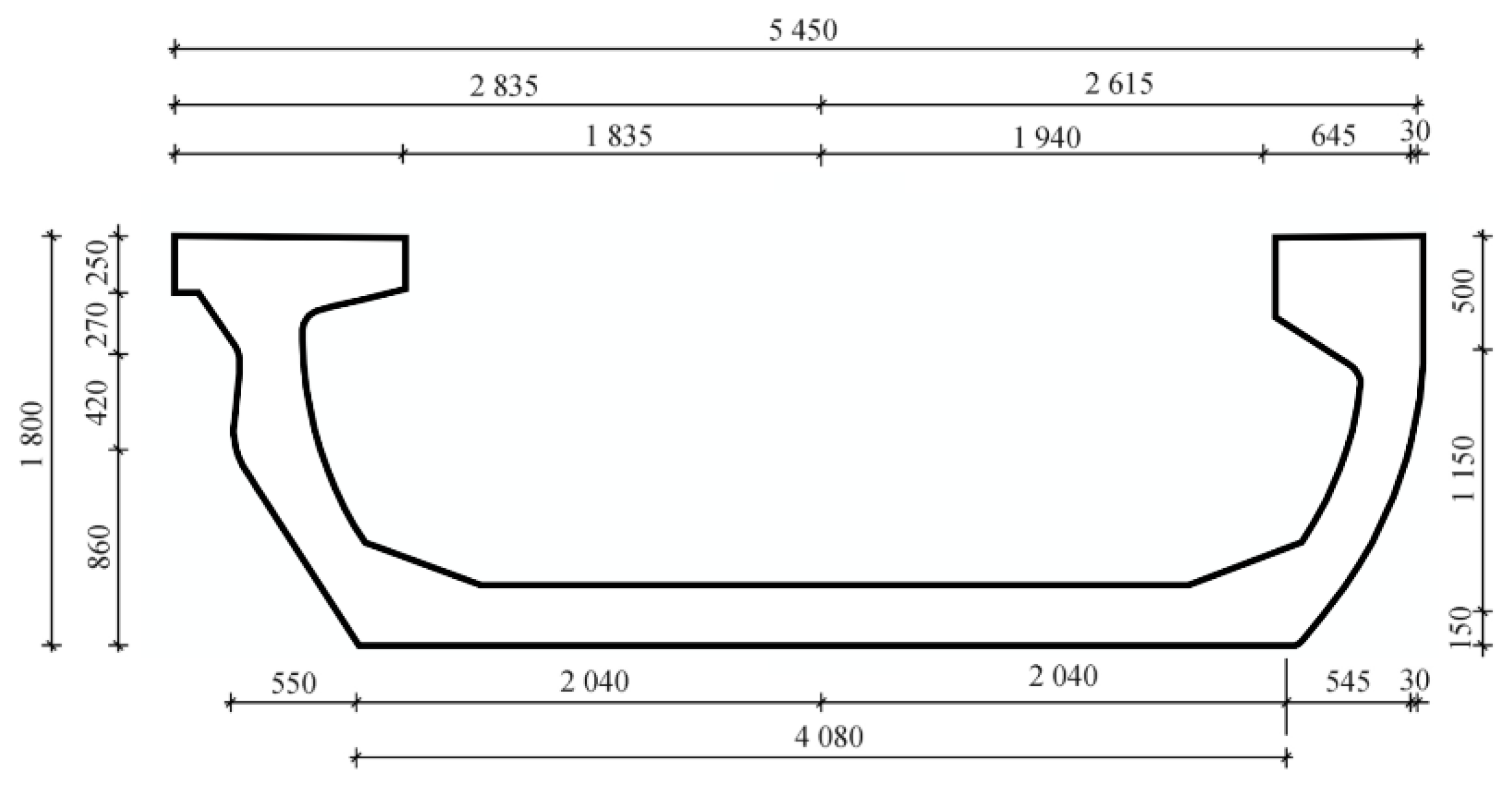
2. Description of U-Shaped Girder Bridges

This study uses a U-shaped girder bridge from the elevated section of Qingdao’s Metro Line 11 as the subject of the experiment. This U-shaped girder bridge has a span of 30 m and open thin-walled structures with arc-shaped side girders. The height of the girder is 1.8 m, the width of the girder is 5.45 m at the top and 4.08 m at the bottom. The field test and cross section of the U-shaped girder bridge are shown in Figure 1 and Figure 2, respectively. Due to the thin-walled open characteristics of the U-shaped girder bridge, its side girders and deck are more susceptible to direct solar radiation, resulting in an uneven temperature distribution within the structure. To understand the distribution pattern of the temperature field under solar radiation for U-shaped girder bridges, this study conducted continuous field observations of the temperature field throughout the year and statistically analyzed these data to provide a reference for the temperature performance of U-shaped girder bridges.

3. Theory of Solar Radiation Intensity and Sunshine Temperature Field

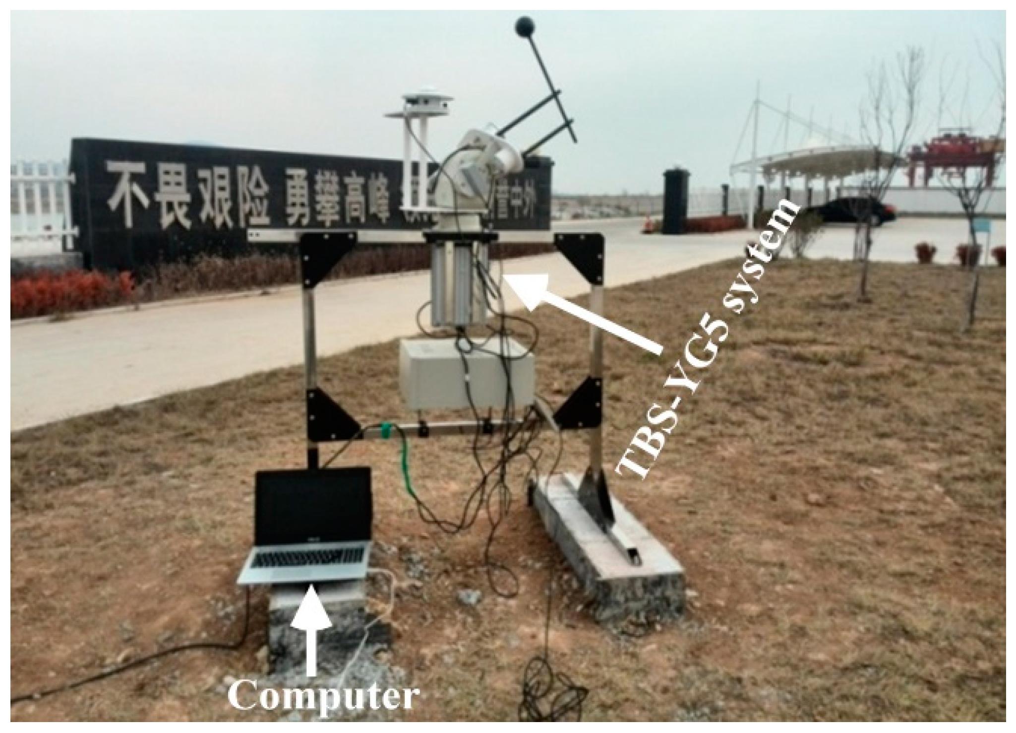
3.1. Solar Radiation Intensity Theory and Test Comparison

3.1.1. ASHRAE Clear Sky Model

The solar radiation intensity is a key factor in calculating the solar-induced temperature field of concrete bridges and is the direct cause of nonlinear temperature stress on structures. The ASHRAE clear sky model [33] is recommended for calculating solar radiation in civil engineering, noted for its simplicity, few parameters, and strong practicality. According to the ASHRAE clear sky model, the solar radiation absorbed by bridge structures includes direct radiation, scattered radiation, and reflected radiation.

Direct radiation: Direct radiation is the solar radiation that reaches the ground directly, and its intensity is as follows:

$$G_D=\frac{A}{\exp (B/\sin \beta )}{C}_N\cos \theta$$

(1)

where A is the solar radiation intensity when the atmospheric mass is 0, B is the atmospheric extinction coefficient, β is the solar elevation angle, C_N represents the atmospheric clarity, and θ is the incidence angle of the sun on the structure surface.

Scattered radiation: Scattered radiation is produced by the scattering of sunlight by molecules and suspended particles in the atmosphere. On the horizontal surface, the intensity of scattered radiation can be expressed as follows:

$$G_{SH}=C\frac{A}{\exp (B/\sin \beta )}{C}_N$$

(2)

where C is the ratio of scatter radiation to direct radiation on the horizontal surface.

For the non-horizontal surface, the intensity of scattered radiation is as follows:

$$G_S=C\frac{A}{\exp (B/\sin \beta )}{C}_N{F}_{ws}$$

(3)

where F_ws is the angular coefficient between the structure surface and the ground.

Reflected radiation: Assuming the surrounding environment is diffusely reflective, ground reflected radiation is the following:

$$G_R=G_{\mathit{tH}}{\rho }_g{F}_{wg}$$

(4)

where G_tH represents the radiation intensity reaching the ground, ρ_g is the reflectance of the surrounding environment, and F_wg is the angle factor for the ground.

Total solar radiation: Total solar radiation is the sum of direct, scattered, and reflected radiation, and can be expressed as follows:

$$G=G_D+G_S+G_R$$

(5)

In practical applications, since the coefficients in the ASHRAE clear sky model are fitted based on actual solar radiation data from the United States, the calculation results cannot be applied directly to China. It is necessary to perform iterative regression on the model coefficients using meteorological data from specific areas to enhance the accuracy of the model. At the U-shaped girder bridge test site, a solar radiation monitoring system, specifically the TBS-YG5 automatic tracking solar radiation, was deployed to observe solar radiation intensity, as depicted in Figure 3. This system monitors and records three parameters continuously: direct radiation, scattered radiation, and the solar elevation angle.

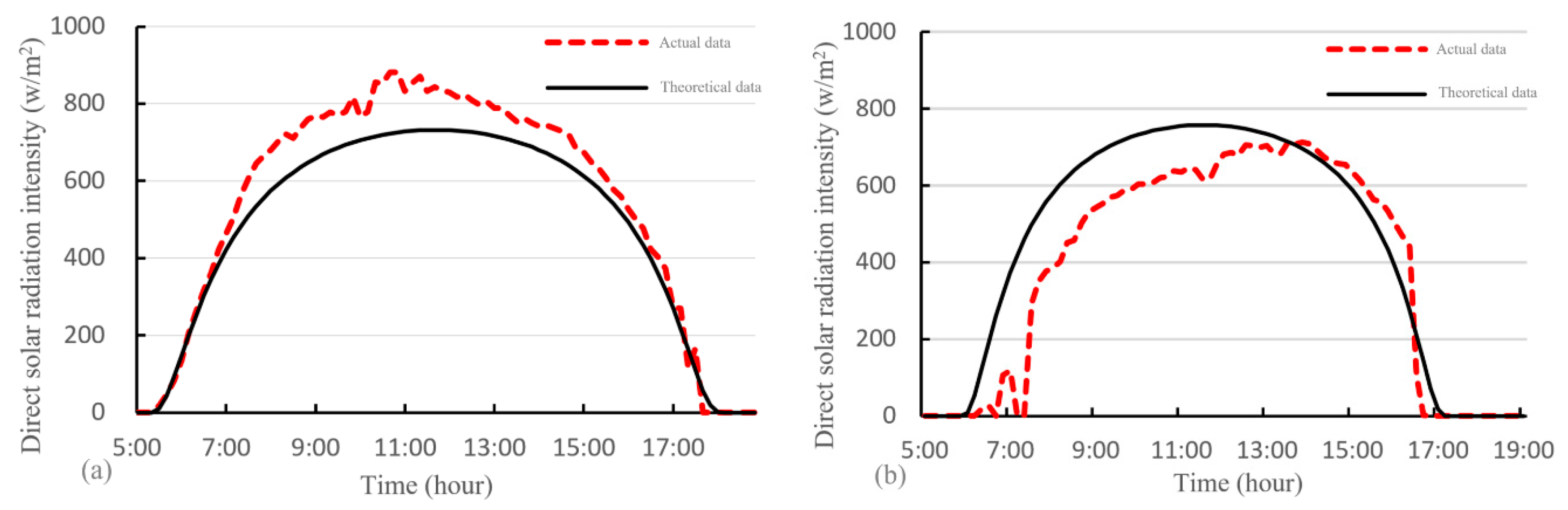
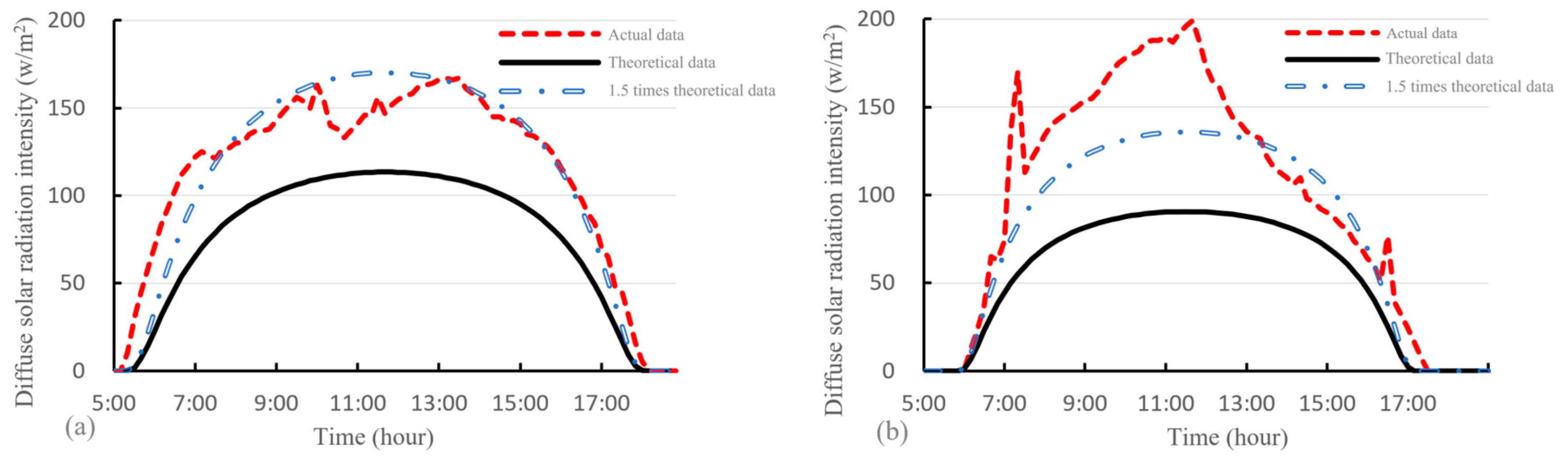
3.1.2. Comparison of Actual and Theoretical Solar Radiation Intensity

In the computation of solar radiation intensity using the ASHRAE clear sky model, it is necessary to choose a series of model parameters that are typically associated with geographic location, atmospheric conditions, and solar position. Li et al. [34] proposed a set of model parameters to describe these conditions, expressed as follows:

$$\{\begin{array}{l}A=1370\left[1+0.034\cos \left(2\pi N/365\right)\right]\\ B=0.2051-4.0537\times {10}^{-4}N+3.5186\times {10}^{-5}{N}^2\\ -1.9832\times {10}^{-7}{N}^3+2.8939\times {10}^{-10}{N}^4\\ C=7.8763\times {10}^{-2}-4.2177\times {10}^{-4}N+1.9908\times {10}^{-5}{N}^2\\ -1.0607\times {10}^{-7}{N}^3+1.5024\times {10}^{-10}{N}^4\end{array}$$

(6)

where N represents the day of the year starting from 1 January. The combined calculation of Equations (1)–(6) can obtain the total solar radiation intensity that can be received at any time and any structural position.

The amount of solar radiation absorbed by concrete structures can be calculated using Equation (7):

$$G_{abs}=\zeta G_t$$

(7)

where G_abs represents the solar radiation absorbed by the concrete structure, G_t is the total radiation intensity on the structure surface, which is related to the vertical incidence angle and direct solar radiation intensity G_D. ζ is the solar radiation absorption coefficient for concrete materials. The shortwave absorption coefficient is 0.65, and the longwave absorption coefficient is 0.88 [34].

During the solar radiation intensity experiment, the study was continuously observed for 365 days. The direct solar radiation intensity was selected for 22 April and 5 October, which are two days that usually present clear weather conditions, ideal for measuring direct solar radiation intensity. The theoretical calculations using the ASHRAE clear sky model were performed, with the comparison of actual and theoretical data illustrated in Figure 4. It can be seen that the actual direct radiation intensity initially shows a small discrepancy when compared to those calculated using the ASHRAE clear sky model in Qingdao, but both exhibit similar trends of variation. This demonstrates that the ASHRAE clear sky model is generally suitable for calculating the direct radiation intensity on U-shaped girder bridges. At the same time, the parameters A, B, and C in the model can adopt the recommended values from the Li-model parameters.

The Li-model parameters were combined with the ASHRAE clear sky model to calculate the theoretical scattered radiation intensity, and were compared with the actual data, with the results shown in Figure 5. The scattered radiation intensity calculated using Li-model parameters and the ASHRAE clear sky model shows considerable deviation from the actual data in Qingdao. This deviation can be attributed to simplifications in the model and variations in instrument calibration. However, multiplying the theoretical scattered radiation intensity by 1.5 results in a close match with the actual data. Therefore, the scattered radiation intensity in the Qingdao area can be calculated by multiplying the theoretical values from the ASHRAE clear sky model based on Li-model parameters by 1.5.

3.2. Sunshine Temperature Field Theory and Test Comparison

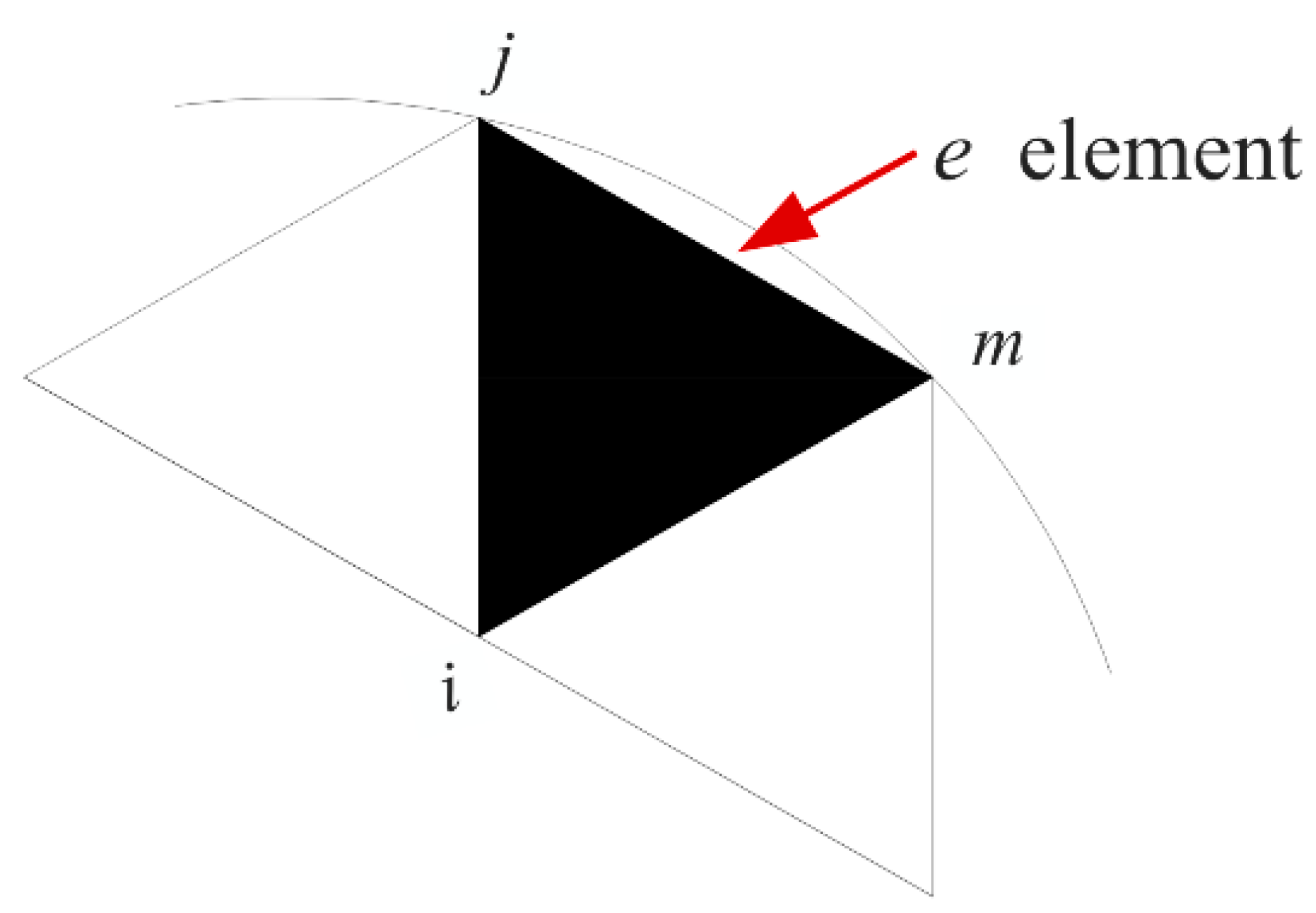
3.2.1. Finite Element Theory of Temperature Fields

The theoretical analysis of the temperature field in concrete structures is complex, primarily involving the accurate depiction of the heat conduction process inside the medium. This process typically follows the Fourier law, which assumes that the material is homogeneous and isotropic in three-dimensional space, explaining the method of heat transfer within materials [35]. For U-shaped girder bridges, the differential equation of the temperature field based on Fourier Law can be expressed as follows:

$$\upsilon \rho \frac{\partial T}{\partial t}=\frac{\partial }{\partial x}(\lambda \frac{\partial T}{\partial x})+\frac{\partial }{\partial y}(\lambda \frac{\partial T}{\partial y})+\frac{\partial }{\partial z}(\lambda \frac{\partial T}{\partial z})$$

(8)

where T is the temperature of the U-shaped girder bridge, λ is the thermal conductivity of the medium, υ is the specific heat of the medium, and ρ is the density of the medium.

Assuming that both web sides and bottom surfaces of the U-shaped girder bridge exchange heat with the environment, the boundary conditions for the temperature field can be expressed as follows:

$$-\lambda \frac{\partial T}{\partial n}=-q+\gamma (T-T_f)$$

(9)

where q represents the rate of heat transfer, γ is the coefficient of thermal exchange, T_f is the specified ambient temperature, and $\frac{\partial T}{\partial n}$ indicates the derivative of T in the direction of the unit normal n to the boundary.

In numerical simulation, two-dimensional triangular thermal elements are often used to simulate the temperature field of bridges, as shown in Figure 6. The finite element equation for the temperature field of the U-shaped girder bridges is established by deriving the thermal equilibrium equation of the two-dimensional triangular thermal element [36].

The node numbers for the triangular thermal element are set as I, j, and m in element e, with each node having only one degree of freedom, which is the temperature a. According to the consistency of the temperature differences at the nodes of element e, the thermal equilibrium equation for element e can be expressed as follows:

$$c^e{\dot{a}}^e+({k_1}^e+{k_2}^e)a^e=p^e$$

(10)

where c^e is the heat capacity matrix, ${k_1}^e$ is the element stiffness matrix, ${k_2}^e$ is the element boundary stiffness matrix, and p^e is the element load matrix.

The total stiffness matrix is formed by aggregating the stiffness matrix of element e; that is, the total heat capacity matrix of the temperature field is [c] = ∑c^e, the total stiffness matrix of the temperature field is [k] = [k₁] + [k₂] = ∑${k_1}^e$ + ∑${k_2}^e$ (the total stiffness matrix of the temperature field includes two parts: the element stiffness matrix and the element boundary stiffness matrix), and the load vector of the temperature field is p = ∑p^e. The finite element equation for the transient temperature field of the U-shaped girder bridge is represented as follows [37]:

$$\left[c\right]\dot{a}+\left[k\right]a=p$$

(11)

where [k] is the total stiffness matrix, a is the total temperature vector, and p is the total load vector.

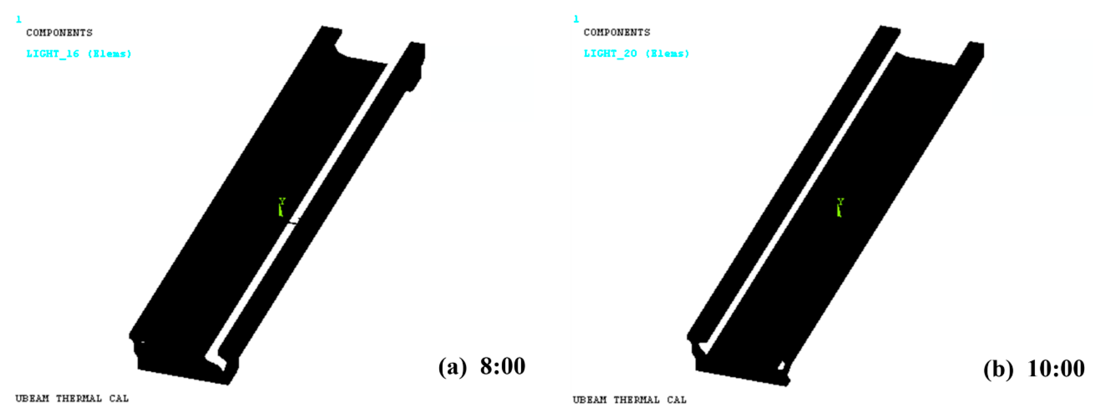
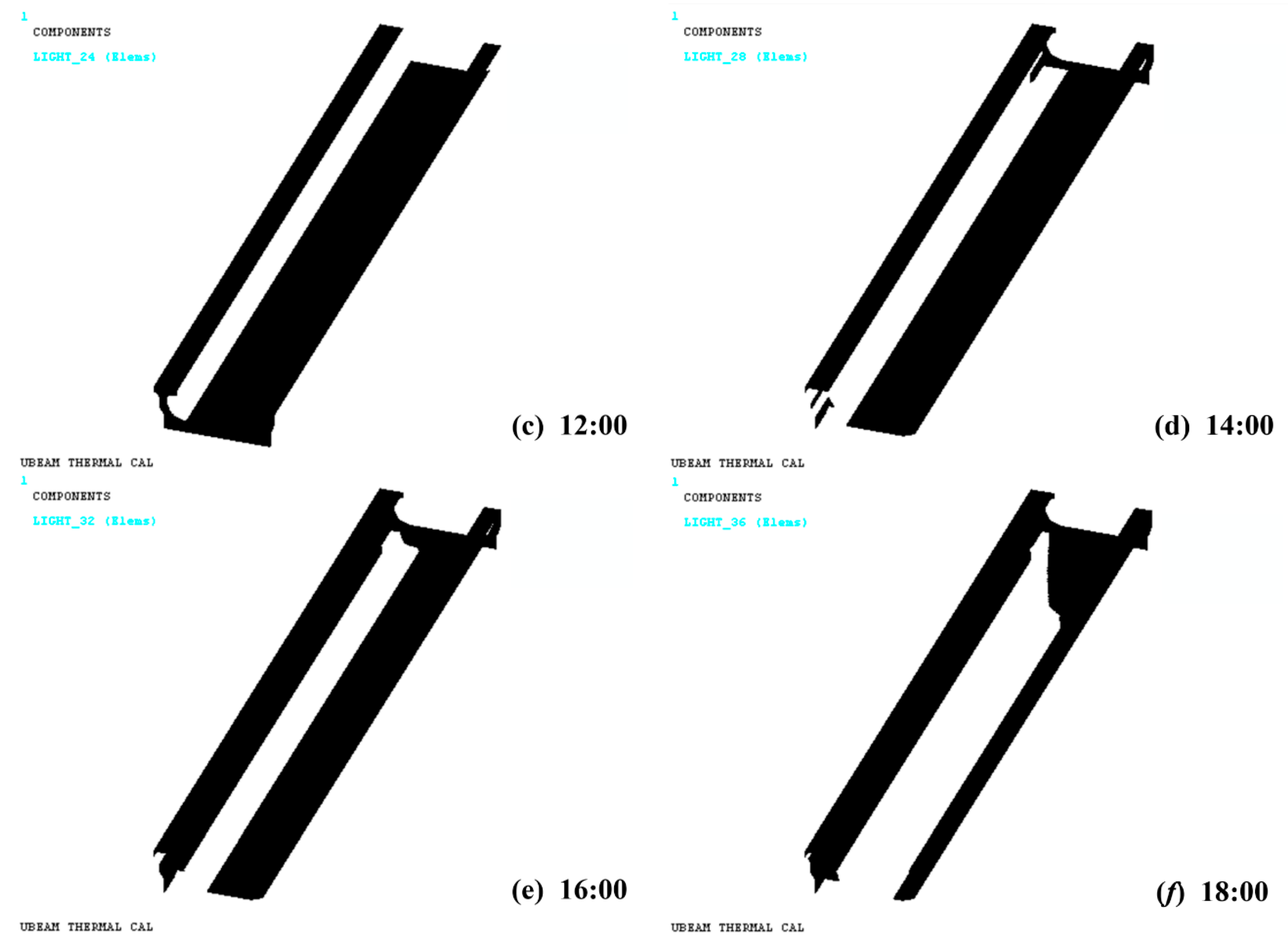
3.2.2. Comparison of Actual and Simulated Shadow Areas

The structure of U-shaped girder bridges is unique, resulting in shading and shadow effects under solar radiation, as illustrated in Figure 7. Since the surfaces of these shadowed areas do not directly receive solar radiation, it is crucial to accurately calculate their impact on the temperature field of U-shaped girder bridges. This study employs a ray tracing algorithm [38,39] to calculate the distribution of sunlight shading in the finite element model of a U-shaped girder bridge.

Figure 8 shows a numerical simulation of the changes in sunlight shadows on the U-shaped girder bridge throughout the day. The black areas represent parts of the U-shaped girder bridge surface that are directly exposed to sunlight, while the white areas indicate parts of the structure that are in shadow. It can be seen that at 8:00, the shadow on the outside of the web is highly consistent with the shadow areas predicted by the numerical simulation. Likewise, the shadows on the inner side of the web at 16:00 are accurately represented through numerical simulation. In general, the shadow areas obtained from numerical simulation are highly consistent with the actual distribution of shadows under sunlight conditions, which not only verifies the effectiveness of the numerical simulation approach but also demonstrates its ability to accurately predict the sunlight conditions of U-shaped girder bridges, including the duration of sunlight and the size of shadow areas. In addition, the numerical simulation not only offers images of shadow distribution at particular moments but also illustrates the dynamic process of shadows throughout the sunlight cycle, supplying data support for analyzing changes in the temperature fields of U-shaped girder bridges.

4. Temperature Finite Element Model and Test Comparison

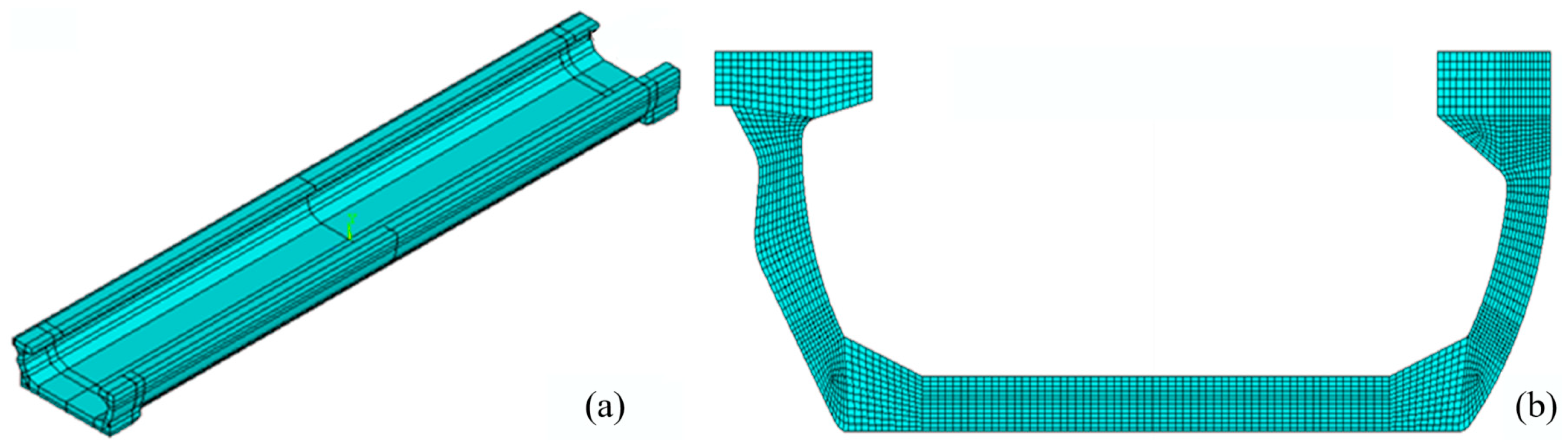
4.1. Temperature Finite Element Model

A three-dimensional transient finite element model (FEM) of the U-shaped girder bridge was established using the ANSYS 16.0 to simulate the temperature distribution under solar radiation effect [40]. The model uses SOLID70 hexahedral heat conduction elements for volumetric meshing to ensure both the accuracy and computational efficiency of the model [41]. The SURF152 elements are used to simulate the surface of the U-shaped girder bridge, allowing for the application of convective and radiative heat loads [42]. In addition, the temperature field shows a nonlinear distribution inside the structure, where high temperatures are only found within a shallow depth of the surface and quickly decrease as the distance from the surface increases. To accurately simulate the nonlinear distribution of the temperature field and ensure computational precision, it is critical to choose the appropriate mesh size. This study selected a mesh size of 5 cm to balance accuracy with the complexity of the calculations. The U-shaped girder bridge comprises a total of 1,690,605 nodes and 1,819,758 elements of SOLID70 and SURF152, and the FEM of the U-shaped girder bridge is shown in Figure 9.

4.1.1. Temperature Field Simulation Parameters

The heat exchange between the surface of a structural surface and the surrounding environment is a complex process in the natural environment, involving radiative heat exchange and convective heat transfer. Radiative heat exchange is typically related to solar radiation, sky radiation, and the radiation from the ground and other objects, while convective heat transfer is mainly related to air in motion. In engineering practice, these two types of heat exchange are usually considered as a combined factor, namely, the comprehensive heat transfer coefficient. Xiao et al. [43] indicates that the comprehensive heat transfer coefficient on the surface of bridges mainly depends on the wind speed at the structural surface, demonstrating the impact of wind speed on heat exchange. As wind speed increases, it leads to an increase in convective heat transfer, enhancing the efficiency of the comprehensive heat transfer. The comprehensive heat transfer coefficient is as follows [43]:

$$h=13.5+3.88v$$

(12)

where v is the wind speed at the structural surface, and h is the comprehensive heat transfer coefficient.

In the numerical simulation of heat exchange for U-shaped girder bridges, parameters such as the density, heat conductivity, and specific heat of concrete are relatively stable and can be determined based on the material of the test bridge and the climatic conditions of the region, with specific values found in

Table 1. Simulation parameters of temperature field.

Simulation Parameter	Density (kg/m3)	Coefficient of Heat Conductivity w/(m·k)	Specific Heat J/(kg·k)	Total Heat Exchange Coefficient h/(m2·k)
Parameter value	2650.0	2.0	930.0	13.5 + 3.88v

. In addition, solar radiation is calculated using the improved ASHRAE clear sky model, and atmospheric temperature and wind speed are based on the standards of the national meteorological administration [44].

4.1.2. Boundary and Initial Conditions for the Temperature Field

Boundary condition settings are crucial in the numerical simulation of the temperature field for U-shaped girder bridges, which specifically include the following four aspects [45]: Shadow area boundary conditions: In the 3D finite element model of U-shaped girder bridges, surface elements in shadowed areas do not receive direct solar radiation, whereas elements within the sunlight areas are exposed to direct solar radiation. Solar scattered radiation: All surface elements of the structure can receive scattered solar radiation. Ground-reflected radiation: Only surface elements that ground-reflected sunlight can reach receive solar-reflected radiation. Radiation and convection between the structure and the atmosphere: For all surface elements of U-shaped girder bridges, the radiation between the structure and the atmosphere is combined with the convective effects, completing the interaction of radiation and convection between the structure and the atmosphere.

The initial conditions need to be set accurately before determining the transient numerical solution of the temperature field of the U-shaped girder bridges [46]; that is, the temperature distribution of the U-shaped girder bridges at the initial moment must be defined. This study adopted a free vibration damping decay mechanism, assuming that the initial temperature field is uniformly distributed. The difference between the initial temperature field set by the model and the actual temperature field will gradually decrease according to an exponential decay pattern. As the computation time increases, this difference will continually decrease, eventually leading the temperature field of the U-shaped girder bridge to converge with the ambient temperature, ensuring the accuracy of the numerical simulation.

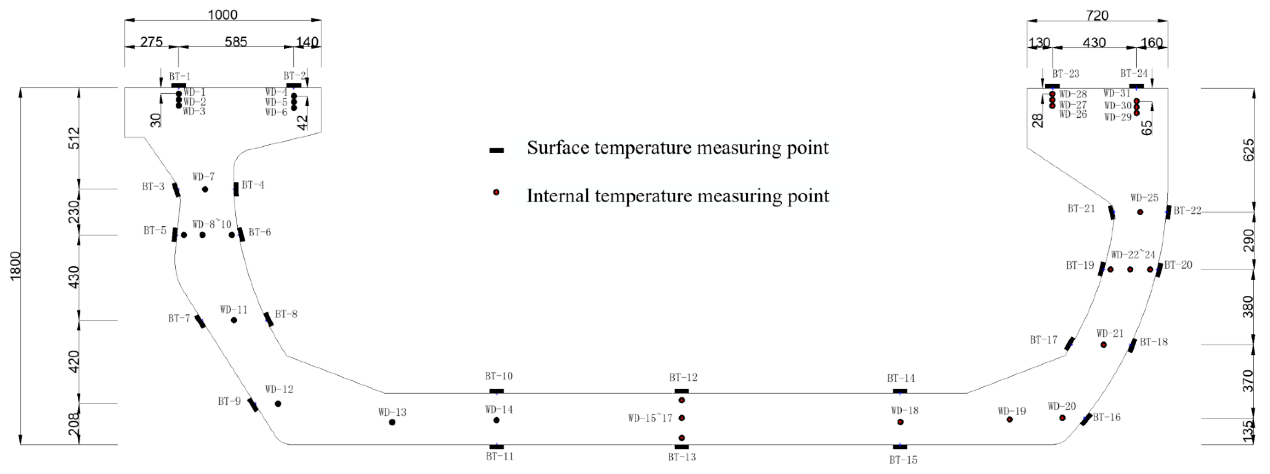
4.2. Distribution of Temperature Sensors

To validate the finite element model of the U-shaped girder bridge, 55 temperature sensors were installed in the midspan cross section, uniformly distributed across the surfaces and interiors of both side webs and the bottom slab. Specifically, 31 temperature sensors were arranged inside, while 24 sensors were positioned on the surface. The top of the webs is affected by daytime sunlight, resulting in significant temperature gradient changes. Therefore, two rows of temperature sensors were arranged longitudinally at the top of the left and right webs, with three in each line and 3 cm between sensors (internal sensors WD1-WD6, WD26-WD31; and surface sensors BT1-BT2, BT23-BT24). The temperature difference in the bottom slab of the U-shaped girder bridges is also very significant, and hence both internal and surface temperature sensors were installed on the bottom slab, namely WD14-WD18 and BT10-BT15, respectively. In addition, these temperature data were collected every 10 min, allowing for 24-h continuous monitoring, with automatic data storage and transmission. The specific arrangement of the temperature sensors is shown in Figure 10.

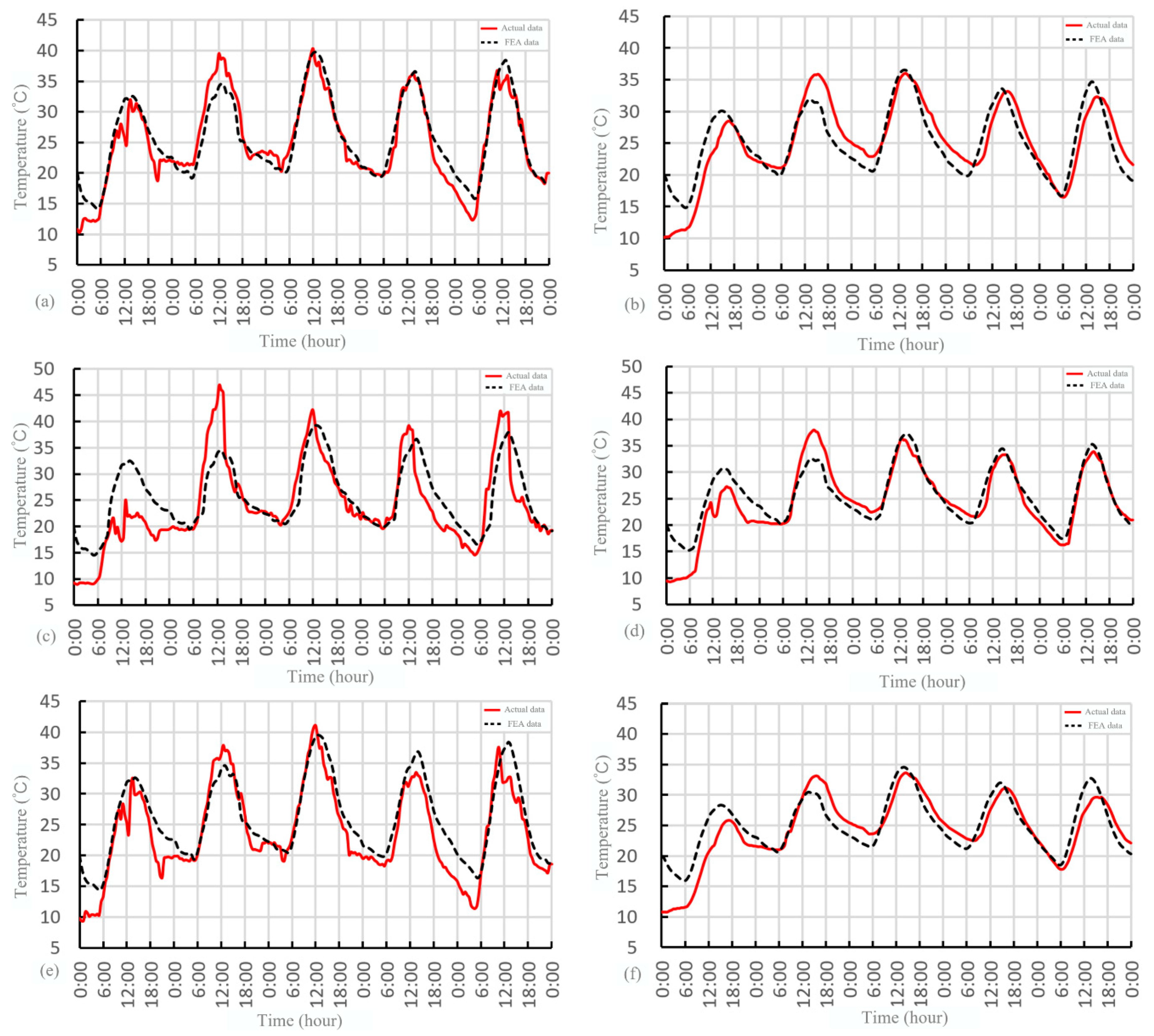
4.3. Test Comparison

Since the numerical simulation conditions for the U-shaped girder bridge had to be consistent with the ASHRAE clear sky model, actual sensor data collected under clear weather conditions were selected for comparative analysis in the simulation. Specifically, the collection of temperature sensor data on the test bridges was carried out on five consecutive days in the warmer months of May and July. During these ten days of observation, all five days in May were clear, while one of the five days in July was cloudy, which still meets the requirement for continuous clear weather. Taking the temperature field of the U-shaped girder bridge for five days in May as an example, the actual data were compared with the numerical simulation results, as shown in Figure 11. It is evident that in the initial two days, although the temperature change trend predicted by the model is roughly in line with the actual data, there are discrepancies in the specific values due to the initial conditions of the finite element model differing from the actual conditions. As the computation time increases, the consistency between the FEM results and the actual data significantly improves after two days, which indicates that the finite element model is consistent with the actual conditions in terms of simulating the heat transfer process with the increase in time.

5. Temperature Distribution of U-Shaped Girder Bridge

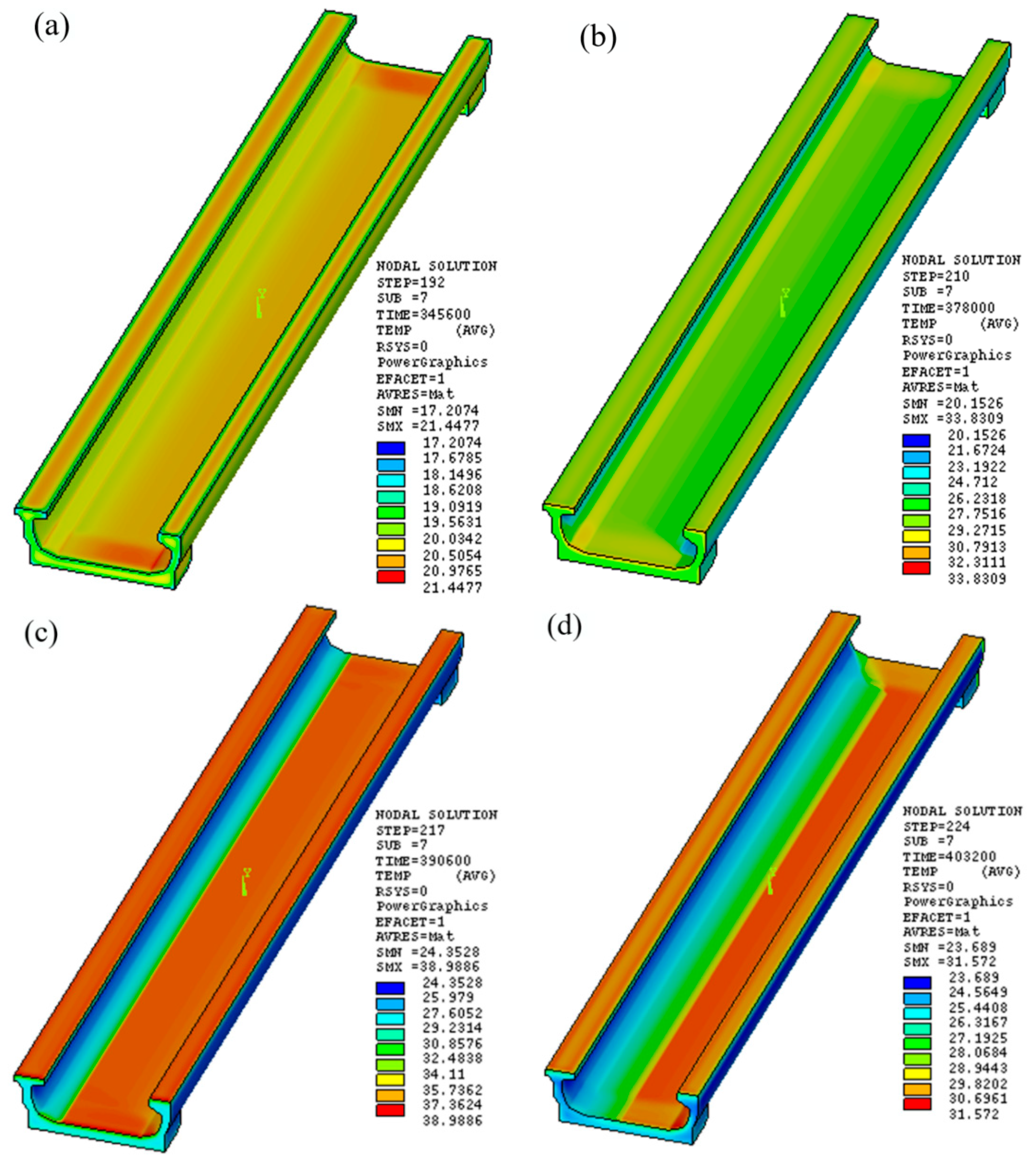
5.1. Three-Dimensional Temperature Distribution

In this section, the FEM U-shaped girder bridge verified by the test was used for numerical simulation of the temperature field, and the results are shown in Figure 12. Figure 12 illustrates the 3D temperature distribution of the U-shaped girder bridge at 0:00, 9:00, 12:00, and 16:00 on 16 May. These times were chosen to depict distinct phases of the temperature cycle of the day. The temperature field has the following characteristics: During the daytime, due to the mutual shading effect of the structure, distinct shadows form on certain areas of the structural surface. The temperatures in these shadowed areas are lower than those in areas exposed directly to sunlight. At the support end of the bridge, the thickened design of the structure and the difference between shadowed areas result in substantial variations in the temperature field compared with other parts of the bridge, but the temperature field changes little along the longitudinal direction. The main reason is the two-way convection effect between these locations and the surrounding temperature, as opposed to a more limited one-way convection effect on other external surfaces, which results in pronounced temperature differences and forms a striped temperature distribution. For example, at 00:00, the temperature at the upper corners on both sides of the web is lower, reflecting the nighttime cooling effect. At 12:00 and 16:00, the temperatures in these areas are relatively higher, related to increased sunlight intensity and heat accumulation.

5.2. Two-Dimensional Temperature Distribution in the Mid-Span Section

Since the temperature field of the U-shaped girder bridge showed little change along the longitudinal direction, while the transverse distribution showed a large temperature variation, the temperature distribution in the transverse section is analyzed in this section. Figure 13 illustrates the temperature distribution across the mid-span section of the U-shaped girder bridge at different times throughout the day. It can be seen that at 12:00, when solar radiation is most intense, the temperature difference across the section also reaches its maximum, approximately 17 °C. At this moment, the temperatures at the upper of the web and the bottom slab are the highest, while the temperatures inside the concrete on both sides of the web are relatively lower. The temperature of the web decreases nonlinearly from top to bottom along its height, and the temperature of the bottom slab gradually decreases along its thickness. At 00:00, the temperature inside the concrete at the upper of the web is relatively high, while the temperature of the outer corners is at its lowest. At the same time, the concrete inside the bottom slab and at the connection between the bottom slab and the webs, known as the haunch, also exhibits higher temperatures. At 16:00, the lateral temperature differences in the bottom slab are notable due to the shading effect of the two sides of the webs, causing part of the bottom slab to be in the shadow while another part is directly exposed to the sunlight, resulting in distinctly different temperature gradients along the transverse direction of the bottom slab. In contrast, at 09:00, the temperature distribution of the structure is more uniform.

5.3. Temperature Distribution of Sensors

In the temperature field test on 14 July, temperature data were collected along the height of the webs, the thickness direction of the bottom slab, and the lateral direction of the bottom slab, and these data were plotted into a temperature distribution, as shown in Figure 14. The temperature fields along the height of the webs and the thickness of the bottom slab exhibit nonlinear changes, while the lateral temperature distribution across the bottom slab is centered around the midspan cross section, showing a symmetrically regular change. In the upper area of the web (0–0.6 m), the FEM prediction results are in good agreement with the actual data, demonstrating the accuracy of the model. However, there are some discrepancies between the actual data and the simulation results in the lower web and bottom slab areas. These differences are primarily due to the moist muddy conditions at the testing site, which influenced the temperature measurement results. Despite these discrepancies, the trend of temperature changes remains consistent between the numerical simulations and the actual data.

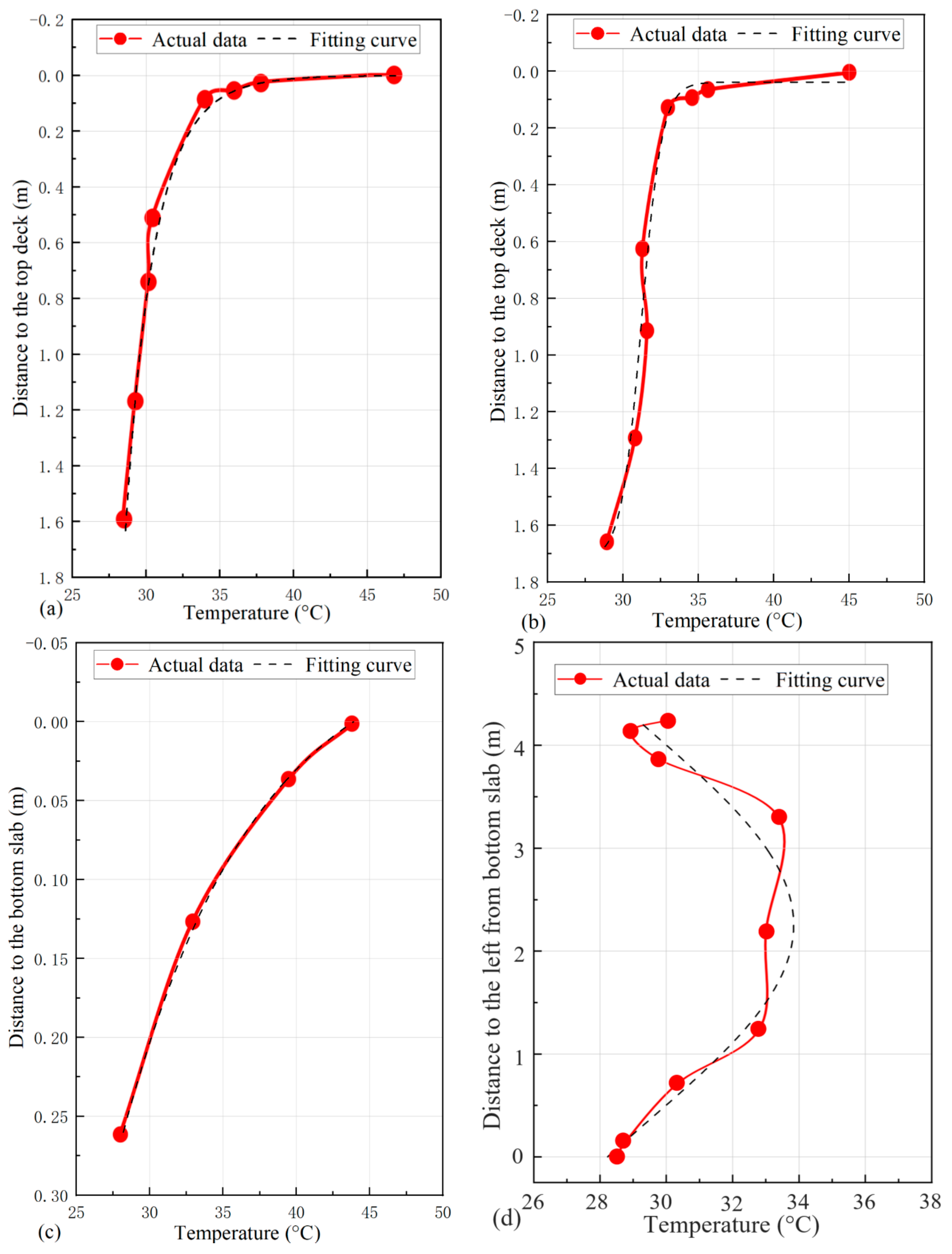
6. Establishment of Temperature Gradient Prediction Model and Test Comparison

The effect of solar radiation on the temperature distribution of U-shaped girder bridges is important, influencing the mechanical properties and durability of the structure. Thus, it is essential for engineering design and maintenance to develop a prediction model that can accurately obtain the temperature gradients in U-shaped girder bridges. By analyzing the actual data in Figure 14, there is a difference in the variation rule of temperature at different parts of the U-shaped girder bridge. To perform rapid temperature gradient calculations, different fitting formulas were applied to each part of the U-shaped girder bridge to predict temperature gradients. For instance, the temperature distribution of the left web was fitted with an Allometricl function to the actual temperature distribution data, as depicted in Equation (13), with related fitting parameters detailed in

Table 2. Allometricl function parameters.

Parameter	a11	b11
Parameter value	4.32 × 1021	−14.71
Standard error	1.50	1.02

. As seen in Figure 15a, the fitted curve closely matches the actual temperature distribution curve of the left web, and the correlation coefficient of the fitted curve is close to 1, with the standard error close to 0, indicating that the Allometricl fitted curve can effectively replace the actual curve for predicting the temperature gradient of the left web. In addition, the temperature distribution of the right web, the thickness direction of the bottom slab, and the lateral direction of the bottom slab can be fitted with the Boltzmann function, sine function, and the inverse transformation of the Gauss function, respectively, as shown in Equations (14)–(16), with these fitting parameters and fitting accuracy shown in

Table 3. Boltzmann function parameters.

Parameter	a21	a22	b21	b22
Parameter value	0.04	1.72	31.23	0.68
Standard error	0.11	0.23	0.28	0.34

,

Table 4. Sine function parameters.

Parameter	a31	a32	b31	b32
Parameter value	38.66	38.65	−1569.50	461.32
Standard error	0.001	0.001	0.02	0.01

,

Table 5. Gauss function parameters.

Parameter	a41	a42	w	x0
Parameter value	2.25	53.16	3.81	22.69
Standard error	0.11	123.62	3.72	15.58

and

Table 6. Fitting accuracy of different functions.

Function	Allometricl	Boltzmann	Sine	Gauss
R2	0.99	0.95	0.99	0.88
Iterations	68	6	60	9

. Comparing the actual data to the fitting curves, these three functions all coincide well with the actual temperature distribution curves. However, there are differences in their fitting accuracy, with correlation coefficients of 0.95 for the right web, 0.99 for the thickness direction of the bottom slab, and 0.88 for the lateral direction of the bottom slab. This is due to the fact that the temperature distribution patterns along the right web and the thickness direction of the bottom slab are relatively simple, resulting in better fitting results. While the lateral temperature distribution of the bottom slab is irregular, making it harder to fit, the Gauss function still fits well in the areas with higher temperatures. Therefore, this study establishes temperature gradient prediction models based on different mathematical functions, which can provide effective computational tools for rapid temperature gradient prediction.

$$y_1=a_{11}\times x_1^{b_{11}}$$

(13)

$$y_2=a_{21}+\frac{a_{22}-a_{21}}{1+e^{\left(x_2-b_{21}\right)/b_{22}}}$$

(14)

$$y_3=a_{31}+a_{32}\times \sin \left[\frac{\pi \times \left(x_3-b_{31}\right)}{b_{32}}\right]$$

(15)

$$y_4=a_{41}\pm w\sqrt{-\frac{1}{2}\log \left[\frac{w\left(x-x_0\right)}{a_{42}\sqrt{\frac{2}{\pi }}}\right]}$$

(16)

7. Conclusions

This study focused on a U-shaped girder bridge to analyze the effect of solar radiation on the distribution of its temperature field using the improved ASHRAE clear sky model and the finite element model. A temperature gradient prediction model for U-shaped girder bridges was developed through nonlinear fitting approaches. The simulation and fitting results of these models were compared with the actual temperature sensor data, and the following conclusions were drawn:

(1)

An improved ASHRAE clear sky model is proposed to simulate the shadow areas of the structure under sunlight conditions, which lays the foundation for numerical simulations of the temperature field of U-shaped girder bridges.

(2)

A three-dimensional transient finite element model of the U-shaped girder bridge is established based on the heat exchange theory, which was used to perform a numerical simulation of the temperature field under solar radiation, comparing the results with actual data. The finite element model results match well with the actual data, verifying the accuracy of the model.

(3)

The finite element model of the U-shaped girder bridge was utilized to analyze the distribution and changing patterns of the temperature field under different solar radiation conditions. The longitudinal temperature change is minimal, while the transverse temperature distribution shows significant temperature gradient changes. Particularly, there are nonlinear changes in the temperature field along the height of the webs and lateral temperature distribution of the bottom slab, with the maximum temperature difference reaching 17 °C.

(4)

A practical calculation method for the temperature gradient is proposed, suitable for predicting the temperature gradient of a U-shaped girder bridge. The model not only has a good fit, but also displays a correlation coefficient with actual data greater than 88%, indicating high prediction accuracy.

The study not only analyzed the characteristics of the temperature distribution of concrete U-shaped girder bridges under solar radiation but also provided an accurate temperature gradient prediction model. However, it is important to note that the applicability of this model is currently limited to the specific geometry of the U-shaped girder bridge. These results are crucial for understanding and predicting the temperature effects on concrete U-shaped girder bridges under solar radiation. Further studies are planned to validate and refine the prediction model proposed in this study under different regions and environmental conditions for a wide range of engineering applications.

References

1. Bai, Y.; Liu, Y.; Liu, J.; Wang, Z.; Yan, X. Research on solar radiation-caused radial temperature difference and interface separation of CFST. Structures 2024, 62, 106151. [Google Scholar] [CrossRef]
2. Li, B.; Nie, Y.; Zhang, J.; Jian, J.; Gao, H. Temperature field of long-span concrete box girder bridges in cold regions: Testing and analysis. Structures 2024, 61, 105969. [Google Scholar] [CrossRef]
3. Li, H.; Ba, Y.K.; Zhang, N.; Liu, Y.J.; Shi, W. Temperature distribution characteristics and action pattern of concrete box girder under low-temperature and cold wave conditions. Appl. Sci. 2024, 14, 3102. [Google Scholar] [CrossRef]
4. Shi, X.; Pan, H.; Liu, Z.; Hu, K.; Zhou, J. Performance of a U-shaped anchoring system for cable-stayed bridges. Structures 2022, 42, 268–283. [Google Scholar] [CrossRef]
5. Junaijath, K.A.; Thomas, J. Effect of inclination of web in the behavior of through type u-girder railway bridges. Adv. Sustain. Constr. Mater. 2021, 124, 613–623. [Google Scholar]
6. Song, X.; Wu, H.; Hao, J.; Cai, C.S. Noise contribution analysis of a U-shaped girder bridge with consideration of frequency dependent stiffness of rail fasteners. Appl. Acoust. 2023, 205, 109280. [Google Scholar] [CrossRef]
7. Zuk, W. Summary Review of Studies Relating to Thermal Stresses in Highway Bridges; Virginia Highway Research Council: Charlottesville, VA, USA, 1965.
8. Erickson, E.L.; Eenam, N.V. Application and development of AASHO specifications to bridge design. J. Struct. Div. 1957, 83, 1320–1331. [Google Scholar] [CrossRef]
9. Churchward, A.; Sokal, Y.J. Prediction of temperatures in concrete bridges. J. Struct. Div. 1981, 107, 2163–2176. [Google Scholar] [CrossRef]
10. Priestley, M.J.N. Thermal gradients in bridges-some design considerations. N. Z. Eng. 1972, 27, 228–233. [Google Scholar]
11. Lu, Y.; Li, D.; Wang, K.; Jia, S. Study on solar radiation and the extreme thermal effect on concrete box girder bridges. Appl. Sci. 2021, 11, 6332. [Google Scholar] [CrossRef]
12. Lin, C.C.; Wang, Y.Q.; Shi, Y.C. Analysis of the temperature field of steel members in sunshine. Steel Constr. 2010, 25, 38–43. [Google Scholar]
13. Emerson, M. The calculation of the distribution of temperature in bridges. Transp. Res. Board Lab. Rep. 1973, 561. [Google Scholar]
14. Hunt, B.; Cooke, N. Thermal calculations for bridge design. J. Struct. Div. 1975, 101, 1763–1781. [Google Scholar] [CrossRef]
15. Mirambell, E.; Aguado, A. Temperature and stress distributions in concrete box girder bridges. J. Struct. Eng. 1990, 116, 2388–2409. [Google Scholar] [CrossRef]
16. Elbadry, M.M.; Ghali, A. Temperature variations in concrete bridges. J. Struct. Eng. 1983, 109, 2355–2374. [Google Scholar] [CrossRef]
17. Branco, F.A.; Mendes, P.A. Thermal actions for concrete bridge design. J. Struct. Eng. 1993, 119, 2313–2331. [Google Scholar] [CrossRef]
18. Imbsen, R.A.; Vandershaf, D.E.; Schamber, R.A.; Nutt, R.V. Thermal Effects in Concrete Bridge Superstructures; National Cooperative Highway Research Program: Washington, DC, USA, 1985. [Google Scholar]
19. Wang, Z.Q.; An, L.Q. Adaptive finite element method for temperature field analysis. J. Eng. Therm. Energy Power 2002, 17, 92–94. [Google Scholar]
20. Liang, Z.; Zhou, H.; Zhao, C.; Wang, F.; Zhou, Y. Experimental and numerical study of the influence of solar radiation on the surface temperature field of low-heat concrete in a pouring block. Buildings 2023, 13, 1519. [Google Scholar] [CrossRef]
21. Sun, R.H.; Ren, W.X.; Yang, X.; Wang, M.Y. Study of two-dimensional temperature gradient of multi-room concrete box girder. J. Hefei Univ. Technol. 2016, 39, 1680–1687. [Google Scholar]
22. Hossain, T.; Segura, S.; Okeil, A.M. Structural effects of temperature gradient on a continuous prestressed concrete girder bridge: Analysis and field measurements. Struct. Infrastruct. Eng. 2020, 16, 1539–1550. [Google Scholar] [CrossRef]
23. Lee, J.-H.; Kalkan, I. Analysis of thermal environmental effects on precast, prestressed concrete bridge girders: Temperature differentials and thermal deformations. Adv. Struct. Eng. 2012, 15, 447–459. [Google Scholar] [CrossRef]
24. Xue, S.; Dai, G.L.; Yan, B. Sunshine temperature mode of prestressed concrete bridge with U-shape section. Sci. Sin. 2016, 3, 286–292. [Google Scholar]
25. Giussani, F. The effects of temperature variations on the long-term behavior of composite steel-concrete beams. Eng. Struct. 2009, 31, 2392–2406. [Google Scholar] [CrossRef]
26. Hagedorn, R.; Martí-Vargas, J.R.; Dang, C.N.; Hale, W.M.; Floyd, R.W. Temperature gradients in bridge concrete I-girders under heat wave. J. Bridge Eng. 2019, 24, 04019077. [Google Scholar] [CrossRef]
27. Wei, X.C.; Zhang, H.S.; Liu, Y.F. Thermal effect on dynamic characteristics of concrete girder bridges. Structures 2024, 61, 105974. [Google Scholar] [CrossRef]
28. Ngo, D.Q.; Nguyen, H.C. Monitoring and analysis of temperature distribution in reinforced concrete bridge box girders in Vietnam. Case Stud. Constr. Mater. 2024, 20, e02857. [Google Scholar] [CrossRef]
29. Yang, X.; Zhou, Y.; Li, X.; Zhang, J. Effect of temperature changes on bearing motion of long-span steel truss continuous girder bridge. Constr. Build. Mater. 2024, 430, 136440. [Google Scholar] [CrossRef]
30. Luo, Q. Temperature Field Test and Theoretical Study of Concrete U-Shaped Beams for Rail Transit; Southeast University: Nanjing, China, 2013; pp. 1–82. [Google Scholar]
31. Liu, W.S.; Dai, G.L.; Rao, S.C. Numerical calculation on solar temperature field of a cable-stayed bridge with U-shaped section on high-speed railway. J. Cent. South Univ. 2014, 21, 3345–3352. [Google Scholar] [CrossRef]
32. Peng, Y.; Zhao, C.; Wang, S.; Zhou, Y.; Xiang, X.; Feng, Y. Mechanical behaviors of the U-girder for urban maglev transit under temperature loads and train loads. J. Vib. Control 2023, 10, 10775463231214822. [Google Scholar] [CrossRef]
33. Mendyl, A.; Mabasa, B.; Bouzghiba, H.; Weidinger, T. Calibration and validation of global horizontal irradiance clear sky models against mcclear clear sky model in morocco. Appl. Sci. 2022, 13, 320. [Google Scholar] [CrossRef]
34. Li, J.P.; Song, A.G. Compare of clear day solar radiation model of Beijing and Ashare. J. Cap. Norm. Univ. Nat. Sci. Ed. 1998, 19, 37–40. [Google Scholar]
35. Sene, N. Second-grade fluid with Newtonian heating under Caputo fractional derivative: Analytical investigations via Laplace transforms. Math. Model. Numer. Simul. Appl. 2022, 2, 13–25. [Google Scholar] [CrossRef]
36. Sun, Y.; Du, C.; Gong, H.; Li, Y.; Chen, J. Effect of temperature field on damage initiation in asphalt pavement: A microstructure-based multiscale finite element method. Mech. Mater. 2020, 144, 103367. [Google Scholar] [CrossRef]
37. Wang, G.C.; Zhang, J.; Kong, X. Study on passenger comfort based on human–bus–road coupled vibration. Appl. Sci. 2020, 10, 3254. [Google Scholar] [CrossRef]
38. Schüßler, C.; Hoffmann, M.; Bräunig, J.; Ullmann, I.; Ebelt, R.; Vossiek, M. A realistic radar ray tracing simulator for large MIMO-arrays in automotive environments. IEEE J. Microw. 2021, 1, 962–974. [Google Scholar] [CrossRef]
39. Kasdorf, S.; Troksa, B.; Key, C.; Harmon, J.; Notaroš, B.M. Advancing accuracy of shooting and bouncing rays method for ray-tracing propagation modeling based on novel approaches to ray cone angle calculation. IEEE Trans. Antennas Propag. 2021, 69, 4808–4815. [Google Scholar] [CrossRef]
40. Soliman, A.S.; Xu, L.; Dong, J.; Cheng, P. Numerical investigation of a photovoltaic module under different weather conditions. Energy Rep. 2022, 8, 1045–1058. [Google Scholar] [CrossRef]
41. Cheng, W.; Chentian, Z.; Shuo, L.; Jianhua, L. Study on Sunshine Stress Effect of Long-Span and Wide Concrete Box Girder. Int. J. Photoenergy 2022, 1, 8149765. [Google Scholar] [CrossRef]
42. Liu, C.; Xiao, J.; Ma, K.; Xu, H.; Shen, R.; Zhang, H. Experimental and numerical investigation on the temperature field and effects of a large-span gymnasium under solar radiation. Appl. Therm. Eng. 2023, 225, 120169. [Google Scholar] [CrossRef]
43. Xiao, J.Z.; Song, Z.W.; Zhang, C.Z. On sensitivity of thermal parameters for concrete box girder in the sunshine. Key Eng. Mater. 2008, 385, 825–828. [Google Scholar] [CrossRef]
44. TB 10002-2017; Code for Design on Railway Bridge and Culvert. China Railway Publishing House: Beijing, China, 2017.
45. Lu, H.; Hao, J.; Zhong, J.; Wang, Y.; Yang, H. Analysis of sunshine temperature field of steel box girder based on monitoring data. Adv. Civ. Eng. 2020, 1, 9572602. [Google Scholar] [CrossRef]
46. Sheikholeslami, M. Numerical analysis of solar energy storage within a double pipe utilizing nanoparticles for expedition of melting. Sol. Energy Mater. Sol. Cells 2022, 245, 111856. [Google Scholar] [CrossRef]
Figure 1. Field test of U-shaped girder bridge.
Applsci 14 06167 g001
Figure 2. Cross section of the U-shaped girder bridge (mm).
Applsci 14 06167 g002
Figure 3. TBS-YG5 automatic solar radiation monitoring system.
Applsci 14 06167 g003
Figure 4. Comparison between actual and theoretical direct radiation intensities: (a) 22 April; (b) 5 October.
Applsci 14 06167 g004
Figure 5. Comparison between actual and theoretical scattered radiation intensities: (a) 22 April; (b) 5 October.
Applsci 14 06167 g005
Figure 6. Two-dimensional triangular thermal element.
Applsci 14 06167 g006
Figure 7. Partial shading of the U-shaped girder bridge at representative times: (a) the outer shadow of the web at 08:00; (b) the inner shadow of the web at 16:00.
Applsci 14 06167 g007
Figure 8. Partial shading FEM model of the U-shaped girder bridge: (a) 8:00; (b) 10:00; (c) 12:00; (d) 14:00; (e) 16:00; (f) 18:00.
Applsci 14 06167 g008aApplsci 14 06167 g008b
Figure 9. Finite element model of the U-shaped girder bridge: (a) three-dimensional model; (b) cross section.
Applsci 14 06167 g009
Figure 10. Arrangement of temperature sensors.
Applsci 14 06167 g010
Figure 11. Comparison between actual and FEM temperature fields: (a) BT1 sensor position; (b) WD1 sensor position; (c) BT10 sensor position; (d) WD15 sensor position; (e) BT24 sensor position; (f) WD31 sensor position.
Applsci 14 06167 g011
Figure 12. Temperature distributions of the U-shaped girder bridge at different times: (a) 0:00; (b) 9:00; (c) 12:00; (d) 16:00.
Applsci 14 06167 g012
Figure 13. Mid-span section temperature distributions at different times: (a) 0:00; (b) 9:00; (c) 12:00; (d) 16:00.
Applsci 14 06167 g013
Figure 14. Mid-span section temperature distributions: (a) left web; (b) right web; (c) thickness of the bottom slab; (d) lateral direction of the bottom slab.
Applsci 14 06167 g014
Figure 15. Comparison of temperature distribution curves: (a) left web; (b) right web; (c) thickness of the bottom slab; (d) lateral direction of the bottom slab.
Applsci 14 06167 g015