Abstract
Given the rapid construction of freeways in developing countries such as China, land use is constantly under strict constraints, leading to challenges in adopting conventional layouts for interchanges. Implementing right-turn ramps on the left (RTRL) at interchanges can minimize land occupancy; however, the traffic safety level in this type of diversion area design requires extra attention. This study examines the decision sight distance for right-turn exit ramps on the left side. Utilizing unmanned aerial vehicle (UAV) video and the YOLOv3 target detection algorithm, the original trajectory data of vehicles in the diversion area is extracted. Employing Kalman filtering and Frenet coordinate system conversion reveals microscopic vehicle lane-change patterns, velocities, and time headways. Furthermore, the driving simulation experiment assesses driver behaviors in RTRL, with subjective, task performance, and physiological measure indicators. Ultimately, the range of the decision sight distance is defined, and establishing a calculation model involves determining relevant parameters based on measured data and simulation outcomes. The results indicate potential insufficiencies in the decision sight distance when standardized values are applied to RTRL.
1. Introduction
The construction of freeways not only spurs economic growth but also fosters rapid national development [1]. Interchanges, which serve as pivotal traffic transfer hubs within the freeway network, assume an indispensable role in diverting and merging crossroad traffic, thereby enhancing convenience in people’s lives and yielding substantial social and economic benefits.
With the relentless pace of urbanization, the freeway network is witnessing a steady increase in density, paralleled by a rise in the number of interchanges. This trend is particularly pronounced in developing countries like China, where the expansive footprint and exorbitant costs associated with interchanges have somewhat curtailed the advancement of urban transportation [2]. Consequently, it has become imperative for interchange design and construction to factor in sustainability considerations [3], including footprint reduction, project downsizing, cost optimization, and advancements in pavement materials [4]. Embracing scientific innovation in interchange design and employing unconventional forms, especially in unique circumstances, can significantly mitigate project costs while aligning with evolving traffic demands and future advancements in transportation technology. Presently, certain regions have adopted unconventional design forms, such as RTRL. For instance, this design has been implemented at the Heilongjiang Sanjian Interchange in China. RTRL intersects the right-turn ramp with the left-turn ramp within the same quadrant, permitting vehicles to exit from the left side of the left-turn ramp.
The innovative design of RTRL not only minimizes land usage but also circumvents the extensive demolition of surrounding buildings, thereby mitigating its impact on the environment. Furthermore, it addresses safety concerns arising from the convergence of small traffic streams exiting from the left-hand side of the right-turn ramp into the main traffic flow. Nonetheless, challenges persist in ensuring optimal traffic safety with this ramp-layout configuration. Firstly, RTRL is predominantly implemented in ramp continuous diversion areas, T- and Y-shaped interchange diversion areas, and mainline side continuous exit areas, but diversion areas have historically exhibited high accident rates [5]. Research indicates that 50% of traffic accidents occur during freeway exits, with the highest incidence observed at exit points compared to other interchange locations [6]. Secondly, driving behavior is closely related to road safety [7,8,9,10,11], with behaviors like straight-line driving and deceleration within the diversion area affecting exit traffic safety significantly [12]. RTRL innovatively challenges traditional design conventions by positioning right-turning vehicles from the left side in the forward direction. However, compared to conventional ramp layouts, this approach introduces greater complexity to road conditions with more signage. As a result, drivers may experience confusion during traffic, leading to reduced driving comfort, increased workload, and ultimately impacting traffic safety.
Some scholars have evaluated the safety of exit ramps using actual accident data [13,14,15] or prediction methods to assess collision risk [16,17,18]. However, these approaches have not adequately considered interchange design aspects to enhance traffic safety in diversion areas. Safety within interchange diversion zones is influenced by various factors [19,20], partly due to insufficient decision sight distance at exits, leading drivers to make emergency lane changes only when they are close to the exit. Some studies have proposed an identification sight distance calculation model by examining its practical application in freeway design in different countries [21]. Nevertheless, due to route alignment and structural limitations, controlling the exit-sight distance according to design standards or guidelines can be challenging in certain cases. Additionally, the current definition of sight distance may not always align with drivers’ decision-making processes, highlighting the need to enhance relevant standard regulations [22]. Regarding driver behavior in diversion zones, some scholars have analyzed driving behavior by gathering data on vehicle speeds, trajectories, and deceleration. They have observed variations in driving behavior across different types of diversion zones and among different drivers [23,24,25,26]. Presently, there is scarce literature directly studying relevant indicators and driver behavior characteristics in the context of right-turn ramp left placement at interchanges. Therefore, investigating the left exit decision sight distance for right-turn ramps in conjunction with actual traffic scenarios and driver behavior can enhance relevant design parameters and improve operational efficiency and traffic safety levels in traffic flows under the left-turn ramp configuration.
The purpose of this study is to analyze the vehicle speed, time headway, and lane-changing behavior within the RTRL at the Xi’an X interchange and L interchange. This analysis is achieved by integrating driver behavior simulation experiments with actual traffic data measurements. Furthermore, the traffic behavior characteristics and driving comfort of drivers in RTRL are evaluated quantitatively through a driver behavior simulation experiment. Finally, the decision sight distance calculation model is established. The parameters within this model are determined by combining the measured traffic data and the results of the driver simulation experiments sequentially to propose the recommended values of the decision sight distance of the RTRL under different design speeds.
The remainder of this paper is structured as follows: Section 2 delineates the collection and analysis of the measured data, including the correlation analysis of the three indicators of vehicle speed, time headway, and lane-changing behavior. Section 3 describes the preparation, simulation modeling, process, and results of the driver behavior simulation experiment in detail. The calculation model for the decision sight distance is established, and the calculation results for determining the relevant parameters and recommended values for the decision sight distance based on the model are provided in Section 4. Finally, conclusions are given in Section 5.
2. Data Collection and Analysis
2.1. Data Collection
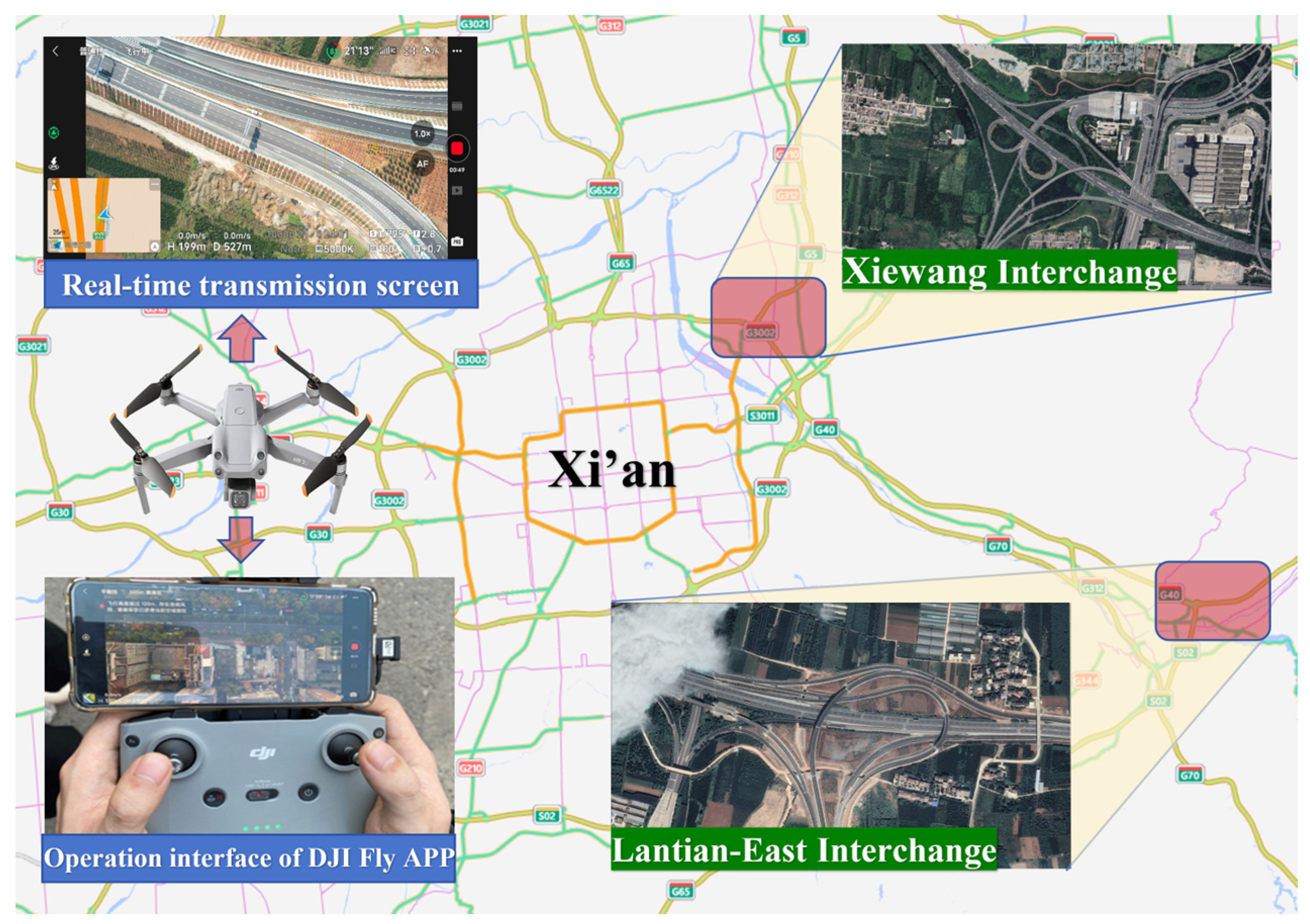
A UAV was deployed to capture aerial video footage of critical sections along the mainline, including deceleration lanes and diversion areas, at the investigated interchanges. For optimal data collection, the chosen locations should exhibit clear weather conditions with minimal wind to ensure unobstructed visibility. Selected shooting sections should also feature comprehensive and distinct signage and markings, free from traffic congestion, accidents, and facility maintenance, thereby minimizing disruptions to drivers.
The UAV employed an advanced O3 mapping solution integrated with the DJI Fly App, facilitating seamless real-time output of high-definition video data. This enhanced the ease of observation for the operator, enabling prompt adjustment of survey parameters as necessary (Figure 1). Throughout the survey process, the UAV ascended to a height of 200 m directly above the designated survey areas, capturing video footage perpendicular to the road sections. Aerial photography sessions were conducted four times during peak hours, with each consecutive session spanning 15 min.

Figure 1.
Data collection sites and devices.
2.2. Data Analysis
The processed aerial video enables the extraction of trajectory data for individual vehicles through analysis using image recognition software. By employing the YOLOv3 target detection algorithm, a trained vehicle detection model facilitates the comprehensive analysis of video frames, facilitating the extraction of crucial vehicle operation data, such as vehicle identification numbers, world coordinates (x and y), vehicle models, and velocities. To ensure data accuracy, anomalous data are meticulously addressed:
- Datasets in which trajectories began and ended nearby, including those encompassing road markings within the detection range, were discarded.
- Iteration through each frame of the vehicle trajectory was conducted to eliminate data points with x-coordinates that were less than their predecessors.
- Vehicle trajectory data located on the paved shoulder were excluded.
Following the aforementioned data-processing methodology, 280 sets of vehicle operation trajectories were obtained. Among these, 78 sets pertained to lane-change trajectory data, comprising 64 sets of right lane changes and 14 sets of left lane changes. Due to the possibility of errors in image detection caused by screen jitter resulting from high-altitude airflow, Kalman filtering was employed to refine trajectory data and minimize decision errors, as illustrated in Equation (1):
where denotes the predicted system state at moment t, and serve as the state transfer matrix. denotes the optimal estimate values of the system state at moment t, denotes the acceleration at moment t, and represent the covariance estimation matrix and the optimal estimation matrix, respectively, is the predicted noise covariance matrix, and the Kalman coefficient is denoted as . The observed matrix and observed noise covariance matrix are represented by and , respectively. denotes the measured position value at moment and , serves as the unit matrix.
Assuming that the state of the system at time is represented by a three-dimensional vector , where signifies the world coordinate, denotes the world coordinate, is the vehicle speed, and is the vehicle speed declination. The state transfer equation is expressed in Equation (2).
The video recording is operated at a frame rate of 30 frames per second, allowing the assumption of negligible vehicle acceleration between consecutive intervals. Consequently, the state transfer matrix is depicted in Equation (3). Additionally, the trajectory prediction curve is based on a third-degree polynomial fit of the scattered data points. This curve ensures a smooth and uninterrupted representation, aligning the vehicle’s instantaneous speed direction tangential to the trajectory curve. Subsequently, the calculation of the vehicle speed deflection angle is presented in Equation (4).
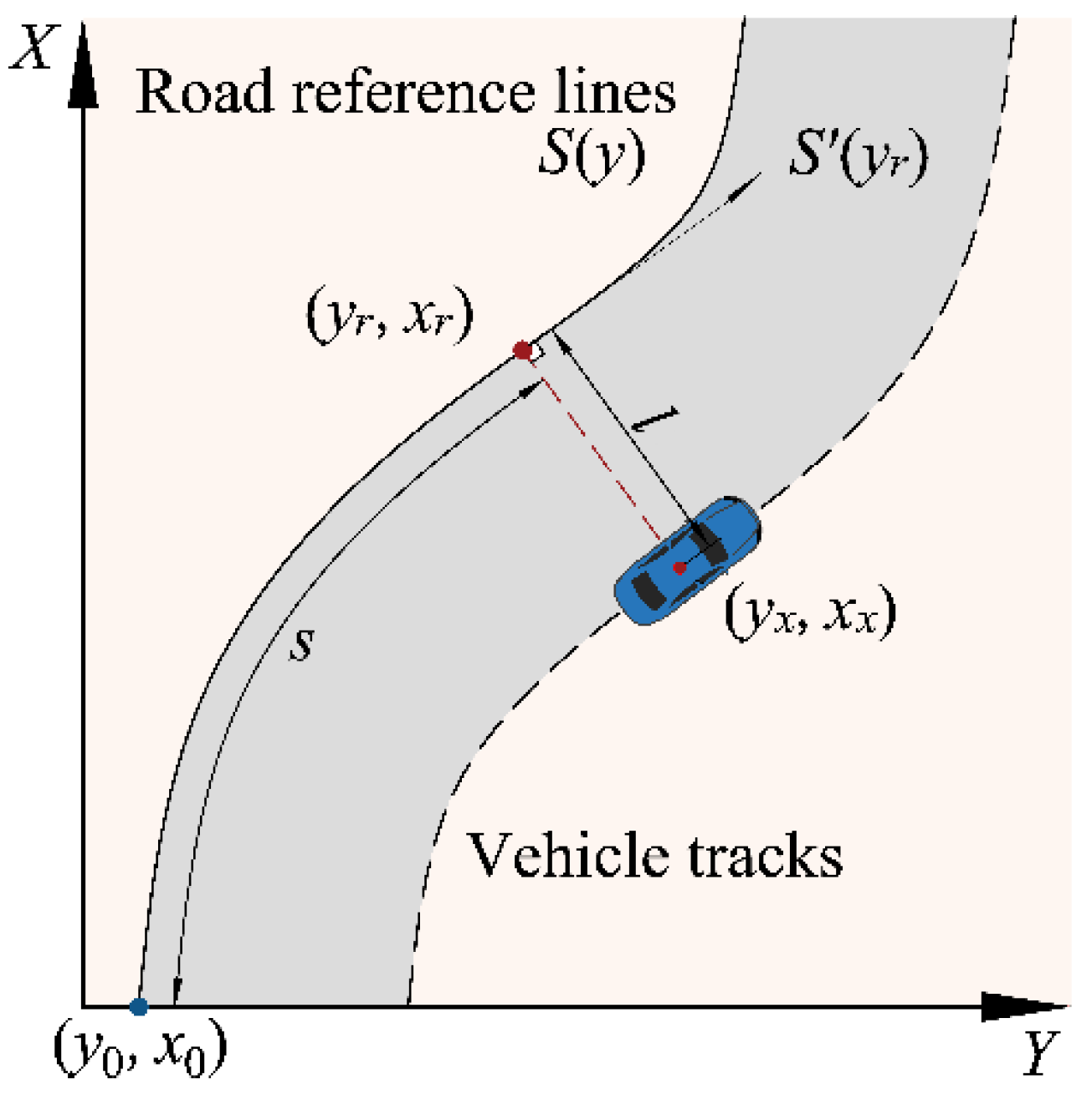
In curved roadway sections, the Frenet coordinate system [27] provides a more intuitive depiction of the vehicle’s relative position on the road compared to the Gaussian plane rectangular coordinate system. The latter features the longitudinal axis S aligned with the road’s centerline, while the transverse axis L is perpendicular to the centerline. Both axes maintain perpendicularity to every point along the road, as visually depicted in Figure 2.

Figure 2.
Coordinate conversion.
The vehicle’s coordinates are denoted as within the Gaussian plane rectangular coordinate system. By considering Equation (5) to locate the nearest reference point on relative to , the vehicle’s position in Frenet coordinates is then determined using Equation(6).
where denotes the longitudinal displacement of the vehicle in the Frenet coordinate system, while signifies the arc length within the Gaussian plane rectangular coordinate system, l indicates the lateral offset distance of the vehicle in the Frenet coordinate system; is the fitted road reference line, and represents the derivative of the road reference line , is vehicle position in Gaussian plane rectangular coordinate system, denotes the closest point to the vehicle position on under the Gaussian plane Cartesian coordinate system.
2.2.1. Vehicle Speed
Spearman’s correlation analysis was conducted on two parameters, vehicle position (m) and vehicle speed (km/h), within Interchange X. The resulting Spearman correlation coefficients are depicted in Figure 3.
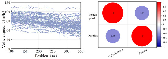
Figure 3.
Vehicle speed distribution and correlation analysis of Interchange X.
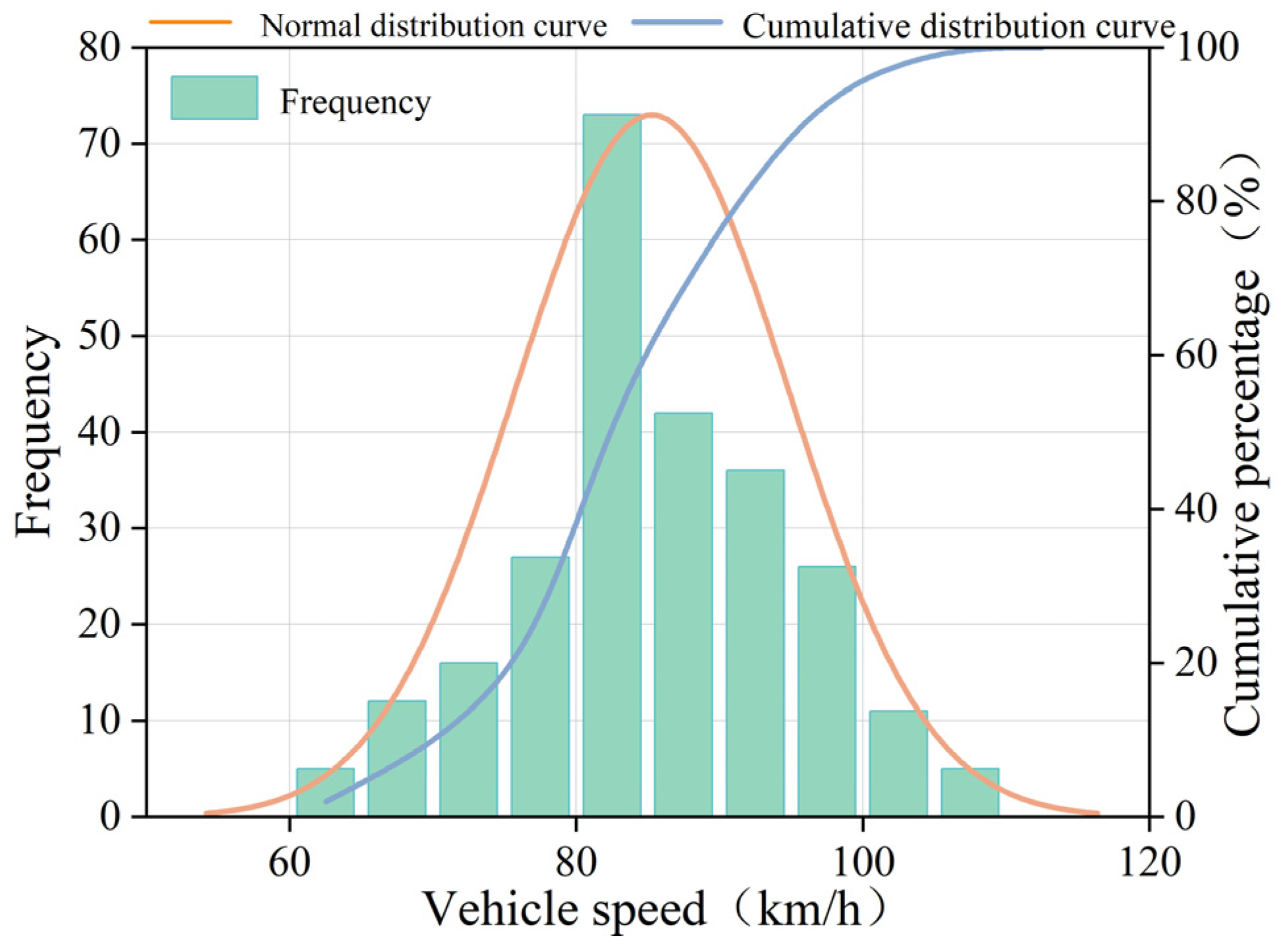
The Spearman correlation coefficient between the vehicle position and vehicle speed within the diversion area of Interchange X was calculated as 0.040. This notably low value suggests a consistent and uniform vehicle speed prevailing in this area. Utilizing Python 3.7 for data analysis, the vehicle speed within the curb lane of the mainline at the initial section of the deceleration lane taper was isolated, resulting in the vehicle speed distribution portrayed in Figure 4.
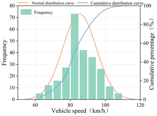
Figure 4.
The vehicle speed of the initial section of the taper.
The speeds measured at the initial section of the taper of the deceleration lane at both Interchange X and Interchange L conform to a statistically significant normal distribution. The average vehicle speed observed at this location and the V85 values are detailed in Table 1.

Table 1.
Characteristic values of vehicle speed at the initial section of the taper of the deceleration lane.
The recorded values from the measured data consistently fall within the range of recommended vehicle speeds designated for the initial section of the taper of the deceleration lane, as specified in Guidelines for Design of Highway Grade-separated Intersections (Intersections Guidelines). Therefore, the upper limit of the recommended interval is adopted as the prescribed value for this indicator due to safety considerations.
2.2.2. Time Headway
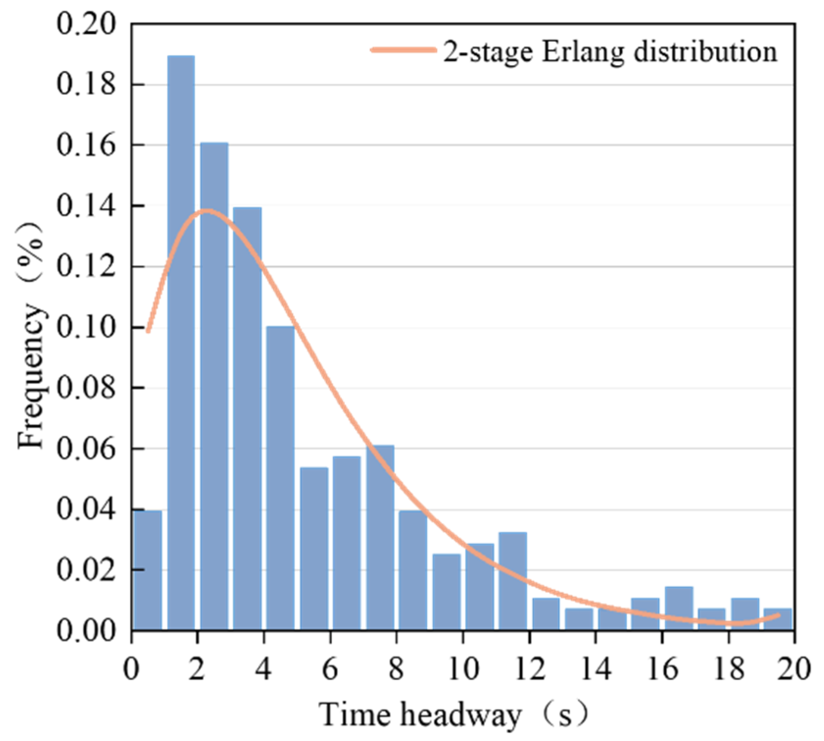
A study has shown that the negative exponential distribution, Erlang distribution, and log-normal distribution can effectively describe the distribution of the time headway [28]. Therefore, the negative exponential distribution, 2-stage Erlang distribution, and 3-stage Erlang distribution were used to fit the measured sample data of the time headway. The adequacy of the fit for each distribution outcome is presented in Table 2.
Table 2.
Results of fitting the time headway for each distribution.
Table 2 demonstrates that the time headway observed in the exit section conforms solely to both the 2-stage Erlang distribution and the negative exponential distribution. Due to the relatively challenging nature of estimating parameters within the negative exponential distribution, the utilization of the 2-stage Erlang distribution is preferred to model the time headway within the exit section of RTRL within the interchange, as illustrated in Figure 5.

Figure 5.
2-stage Erlang distribution fitting time headway at Interchange X.
2.2.3. Lane-Change Behavior
The hyperbolic tangent function lane-change trajectory model is closely linked to driver behavior and provides a better fit for the actual lane-change trajectory [29]. Nevertheless, the model’s expressive range does not fully encompass the function, leading to a discrepancy between the obtained lane-change width through fitting and the actual width. To address this discrepancy, the function model is adjusted by incorporating width boundary conditions, as shown in Equation (7):
where denotes the transverse distance of the lane change (m), represents the transverse position of the vehicle at the moment (m), and signifies the transverse position of the vehicle at the initiation and completion of the lane change (m), corresponds to the longitudinal displacement during lane change, which is the length of the lane change (m), is the longitudinal average vehicle speed in the process of lane change (m/s), stands for the total width of transverse displacement during the lane change (m), is the emergency coefficient of the lane change, while denotes the duration of the lane change (s).
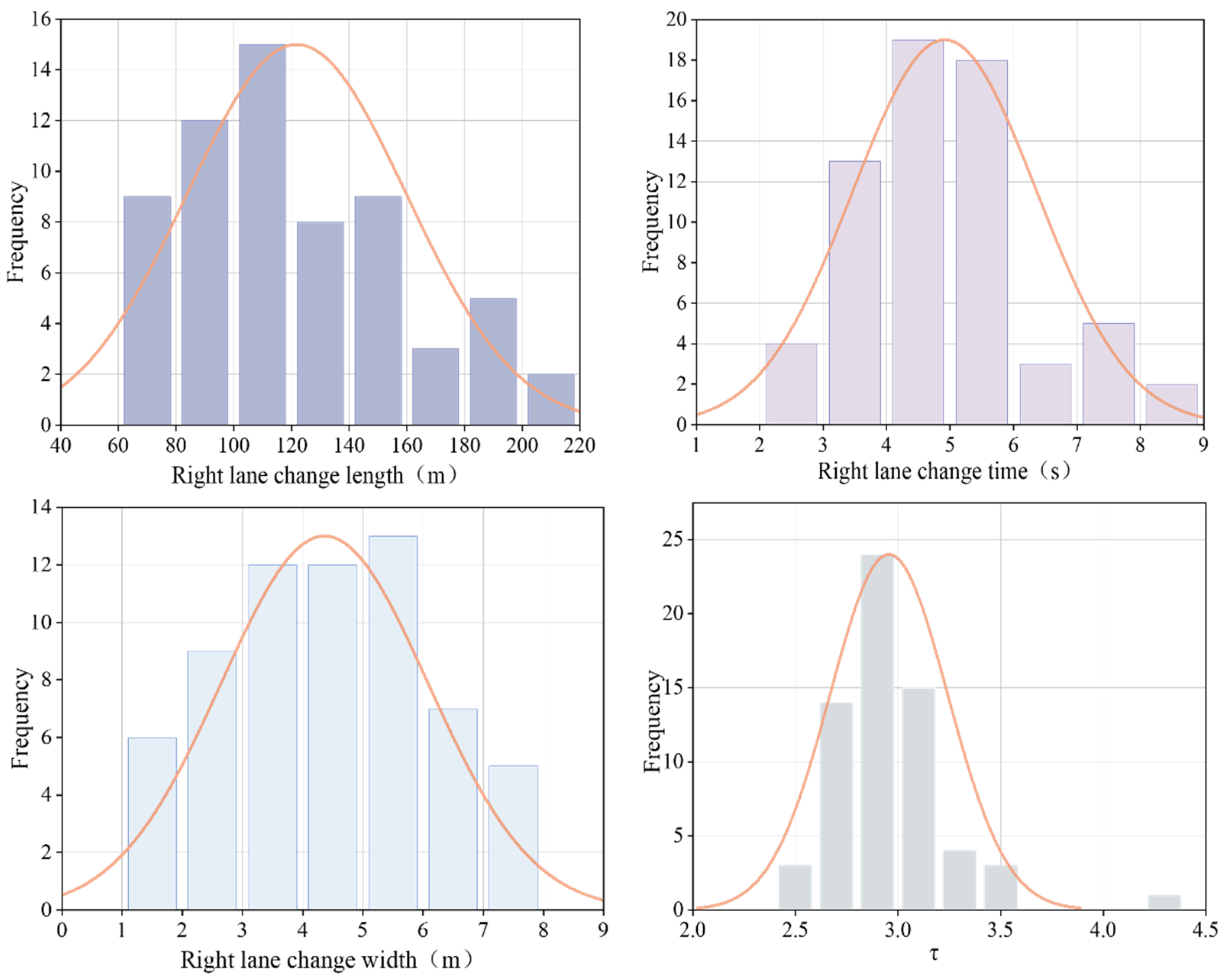
Figure 6 displays the temporal aspects, length, width characteristics, and distribution of the urgency factor derived from 64 instances of lane change to the right side (LCR) observed at Interchange X.
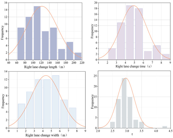
Figure 6.
Parameters related to LCR.
The mean goodness of fit achieved by the Python 3.7 computation for the modified hyperbolic tangent function permutation model applied to the right lane permutation trajectory stands at 97.18%. This result signifies a high degree of feasibility and compatibility of the model with the LCR trajectory. As depicted in Figure 6, τ values for the LCR predominantly range from 2.5 to 3.5. To ensure smooth and safe lane changes for the majority of vehicles navigating the diversion area, it is imperative to set the maximum value of the emergency coefficient of lane change at 3.5.
3. Driver Behavior Simulation
3.1. Determination of Test Apparatus and Personnel
To elucidate drivers’ traffic behavior and visual patterns while navigating RTRL at interchanges and to explore the variations in vehicle speed, visual attributes, and psychological responses of drivers in these sections, which are essential for establishing parameter values in the decision sight distance calculation model, a simulation driving test was collaboratively conducted. This test utilized the UC-win/Road 9.1.0 simulation software, Forum8 driving simulation and emulation platform, and SMI ETGTM spectacle-type eye-tracking device, as depicted in Figure 7.
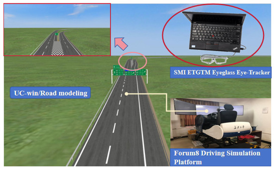
Figure 7.
Driver behavior simulation equipment and 3D scene modeled by UC-win/Road software.
The UC-win/Road software operates on the principles of computer-generated 3D virtual modeling, effectively simulating real-life scenarios and aiding in road traffic design by creating 3D road environments in diverse settings like freeways, urban streets, and tunnels. Meanwhile, the Forum8 driving simulation platform integrates a 3D road model and traffic environment to provide simulated real-world driving scenarios for testing. As drivers execute designated driving maneuvers within the simulated cockpit, the platform captures their visual observations and driving experiential responses, mimicking real driving behaviors. The SMI ETGTM eyeglass eye-tracking instrument monitors the driver’s visual behavior by capturing eye movement characteristics. Key instrument parameters include a sampling frequency of 120 Hz for both eyes, a tracking distance of more than 40 cm, tracking resolution of 0.1°, gaze localization accuracy of 0.5°, and horizontal and vertical field of view angles of 120° and 92°, respectively.
The precision of the test outcomes and subsequent conclusions is directly contingent upon the judicious selection of the test sample size, thereby significantly influencing data collection and result interpretation. Following statistical principles, this experiment employed a two-sided test methodology to ascertain the optimal number of participants required. The calculation of this figure is determined using Equation (8).
where denotes sample size, is the significance level, which was taken as 0.05 in the test, so the confidence level coefficient is calculated as 1.96. represents the probability of committing the second type of error, as indicated by related research, when , the sample data can reflect the overall the test takes 0.1, , signifies the standard deviation, is the difference between the tolerance error and the check, the test takes 9.3.
Based on Equation (8), the calculated minimum sample size necessary for the test amounted to 10 individuals. To ensure both the test’s validity and practicality, considering the gender distribution and driving age of drivers [30], a selection of 12 male drivers and 4 female drivers was made. These participants boasted an average driving experience of 3 years and exhibited a visual acuity of 1.0 or higher. Moreover, to guarantee the quality of the driver eye-gaze data, subjects aged between 23 and 35 years were specifically chosen. Detailed information regarding the test subjects is provided in Table 3.
Table 3.
Basic information on the test personnel.
To maintain the precision of the test results, the following prerequisites were stipulated for the subjects:
- Subjects were required to be in a normal physiological condition before commencing the test.
- Prior simulated driving training was mandatory to ensure complete familiarity with and mastery of the simulated cockpit operation. This training aimed to facilitate adaptation to the differences between a simulated driving environment and that of a real vehicle.
3.2. Scene Modeling and Test Procedure
Based on the road environment and geometric design elements present at a specific interchange (Interchange X) in Xi’an, China, the simulation test employs the UC-win/Road software to construct a comprehensive three-dimensional representation of the roadway. Notably, the primary route of Interchange X, designated for the Jingkun Freeway, supports a vehicle speed of 120 km/h, with four lanes in each direction. Meanwhile, the ramps cater to a vehicle speed of 60 km/h, accommodating two lanes in one direction. The simulation model should emphasize the green surroundings alongside the freeway, as depicted in Figure 8.
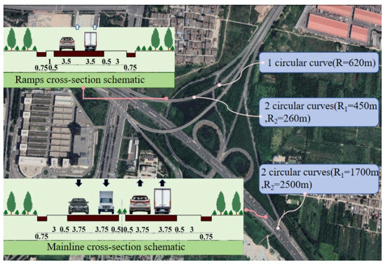
Figure 8.
The RTRL Design of Interchange X.
Figure 9 illustrates the simulation test process. Following the training session, the drivers were briefed on essential details concerning the road section. They were encouraged to adhere to the designated design vehicle speed while driving as closely as possible. Moreover, the subjects were instructed that if they discovered they had chosen the incorrect path, leading to an erroneous travel direction, they were not permitted to stop or turn around at the same location. To reduce potential testing errors, participants were advised to maintain minimal head movement while driving and to adjust their seating position beforehand.
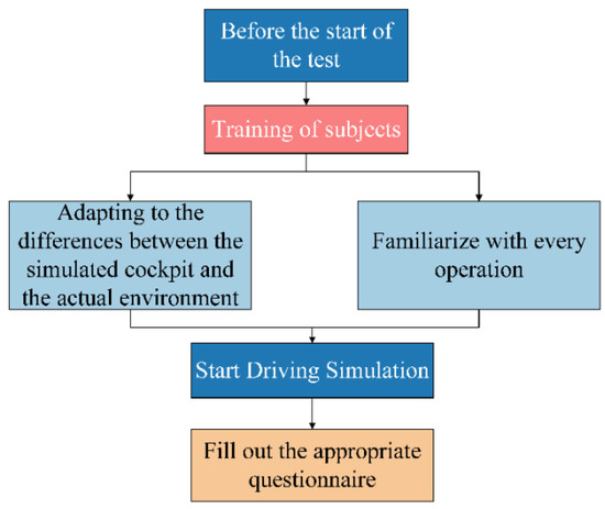
Figure 9.
Simulation test process.
3.3. Driver Accuracy and Comfort
The number of driving errors among the 16 subjects amounted to 2, resulting in a driving error probability of 12.5%. The complexity and abundance of place names exhibited on the signboards guiding toward the Interchange X exit significantly contributed to the subjects’ inability to swiftly extract pertinent information. Consequently, subjects faced challenges in efficiently locating useful information within a limited timeframe. Based on the questionnaires completed by the subjects at the experiment’s conclusion, the summarized feedback regarding comfort is illustrated in Figure 10.
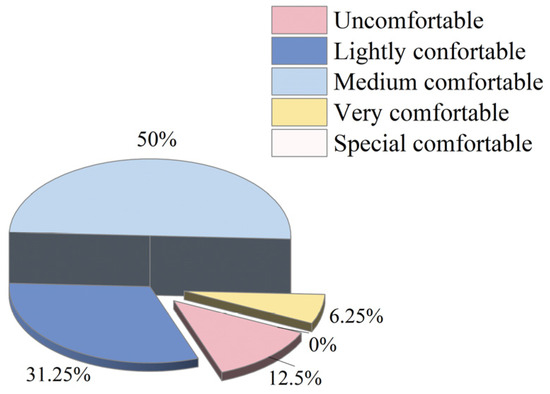
Figure 10.
Driver comfort survey results.
Upon analyzing the questionnaire results, it is evident that RTRL, inadequate signage, and suboptimal continuous diversion spacing in the exit section contribute to the diminished comfort of drivers within this section. Firstly, the unconventional layout of RTRL may perplex drivers during task execution, impacting their ease and accuracy in path judgment compared to traditional ramp layouts. Secondly, improper placement of exit section signage may restrict drivers’ ability to swiftly gather essential road information, potentially causing confusion and affecting their comfort and precision in driving operations. Moreover, insufficiently spaced upstream and downstream continuous exits in the ramp diversion area can impede drivers from executing standardized and safe driving maneuvers, further detracting from driving comfort.
3.4. Driver Workload Measurement and Results
Scholars have discovered that driving induces various loads [31]. Excessive or insufficient driver workload negatively impacts driving safety and efficiency. Optimal driving performance is achieved only within a reasonable workload range. Studies [32] have highlighted three primary methods employed for evaluating driver workload.
- Subjective Measurement
The NASA Load Index (NASA-TLX) scale is employed as the evaluation criterion for subjective measurement. Sixteen NASA-TLX scales and six-dimensional weight comparison cards were obtained. Utilizing the original scores and weights of the six load dimensions, Equation (9) is applied to calculate the subjective driving workload values of the subjects.
The subjective driving workload values of the subjects are shown in Table 4.
Table 4.
Raw scores , weight , and subjective driving workload values for load dimensions .
From Table 4:
- The weightings assigned to the three load dimensions—mental demand, time demand, and effort, are notably substantial, indicating elevated demands on drivers’ cognitive faculties, decision-making skills, and attentiveness caused by RTRL. Simultaneously, ensuring optimal driving efficiency within RTRL necessitates the application of relevant design parameters and signage placement, enabling drivers to have sufficient reaction time for operations.
- The majority of subjects exhibit higher workload values, confirming the escalated complexity involved in the driving task within RTRL.
- 2.
- Task Performance Measures
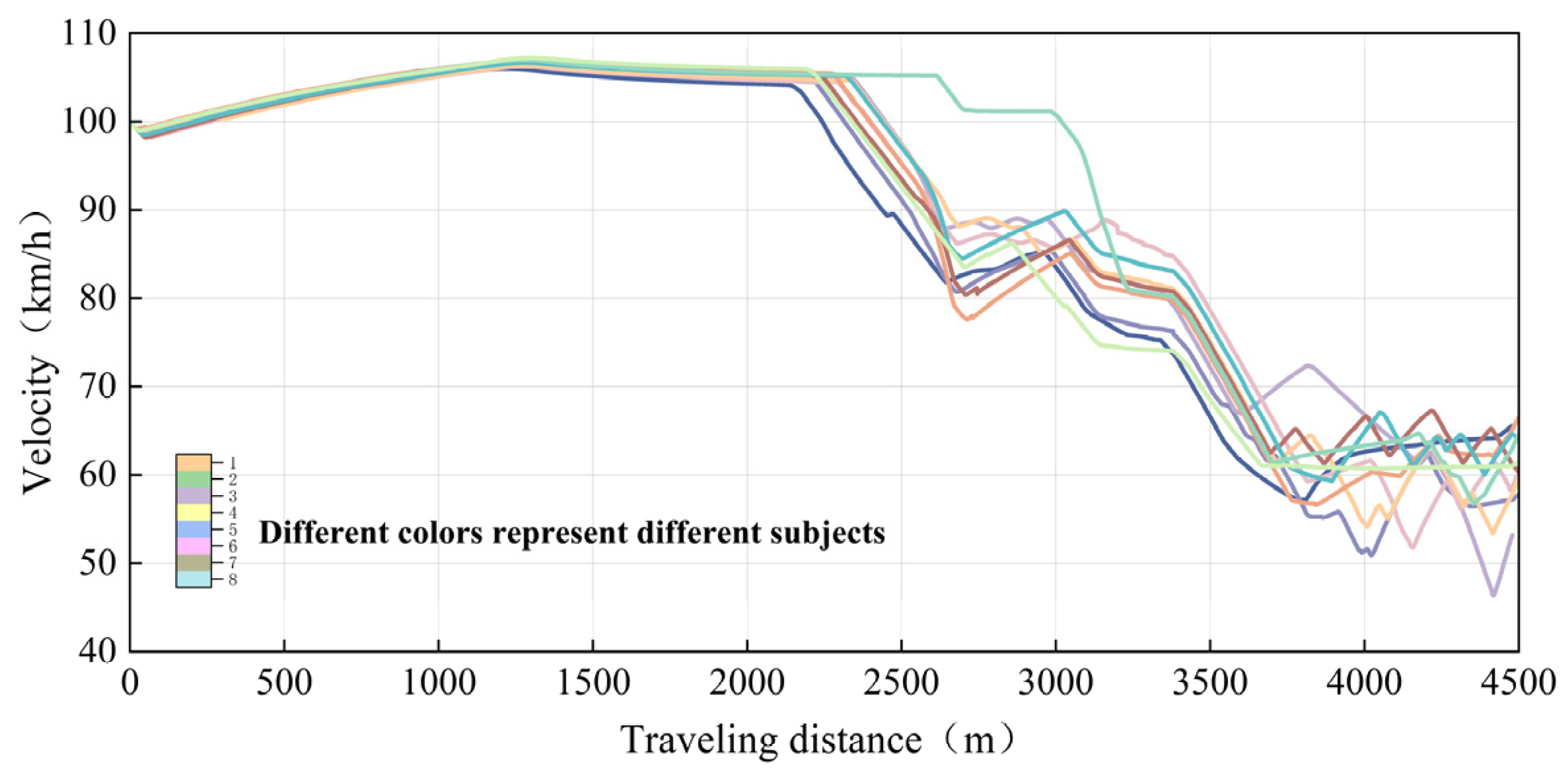
Vehicle speed serves as an intuitive indicator of the impact of the road environment on driver performance. A higher vehicle speed indicates favorable road conditions. Thus, vehicle speed was utilized as a task performance indicator. The UC-win/Road simulation software recorded the vehicle speed, as shown in Figure 11.
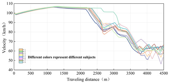
Figure 11.
Distribution of vehicle speed for some subjects.
There is a notable decrease in vehicle speed before the diversion area and at approximately 800 m from the diversion nose (at 3100 m), which prompts subjects to execute the driving task smoothly and calmly. Around 400 m from the diversion nose, a slight vehicle speed increase of 5–8 km/h is observed, which indicates that having clarified the driving direction, subjects began to incrementally increase their speed.
- 3.
- Physiological Measurements
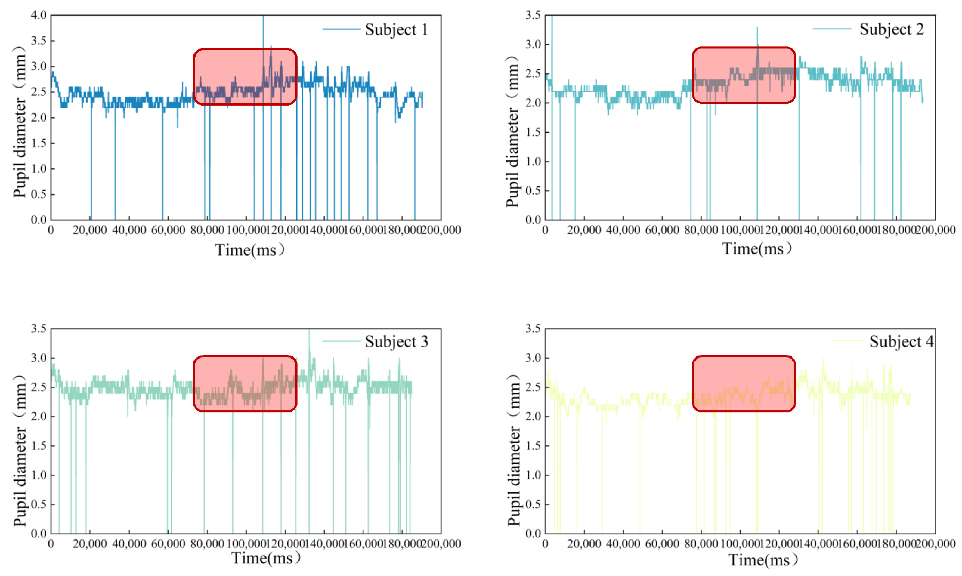
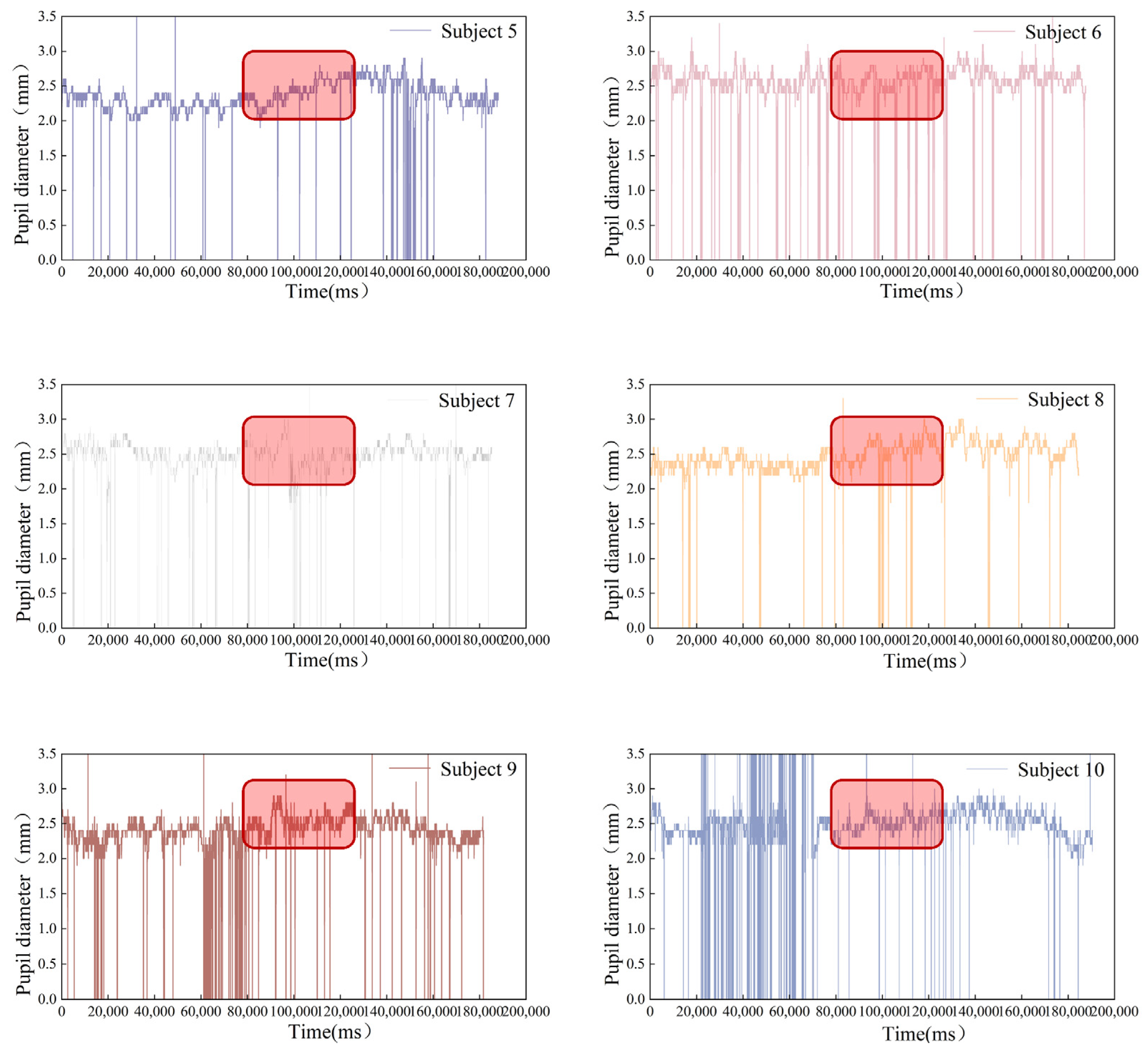
The pupil diameter was chosen as the evaluation index for the physiological measurement method. Subjects’ pupil diameter data were collected using the SMI ETGTM spectacle-type eye-tracking device. BeGaze 3.6.52 analysis software processed the pupil diameters of the subjects in each driving scenario to ascertain the characteristics of their pupil diameter variations. Larger amplitude fluctuations and more frequent pupil diameter fluctuations indicated higher physiological driving loads among the subjects. The changes in the subjects’ pupil diameter data are shown in Figure 12.
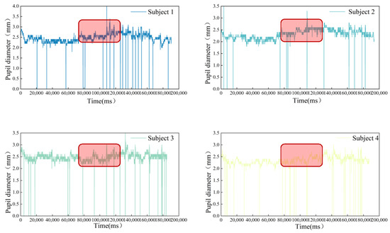
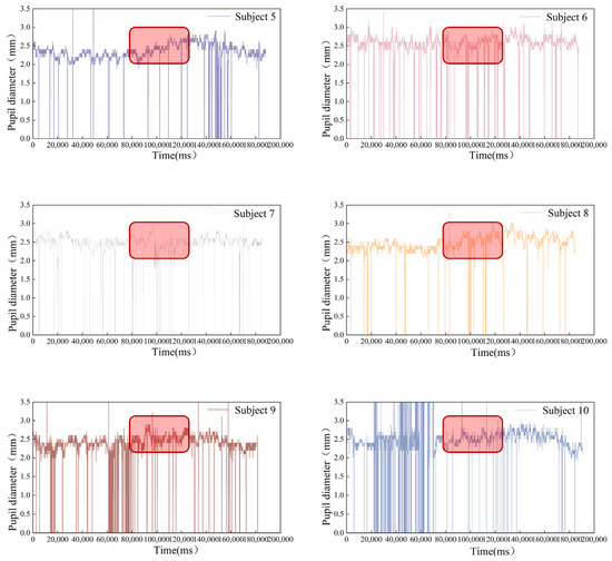
Figure 12.
Changes in pupil diameter in some subjects.
Subjects generally exhibited small pupil diameters, with most displaying an increasing trend and heightened fluctuations in pupil size near the exit (corresponding to a period of 80,000 to 120,000 ms). This suggests that making choices regarding diversion directions in the exit area significantly escalates the mental and physiological loads experienced by drivers. To efficiently perceive overhead road sign information within a constrained time frame, subjects needed to widen their pupil diameters to gather more road-related data. This increase in pupil diameter indicates an elevated physiological burden on the drivers’ hearts within the diversion area, characterized by a left-positioned right-turn ramp.
Furthermore, subjects demonstrated relatively small and stable pupil diameters within the mainline section pre-exit and the ramp section post-exit. This stability implies that subjects in these baseline sections experienced a comparatively more relaxed driving environment compared to those within the traffic diversion area.
4. Calculation and Results
4.1. Calculation Model
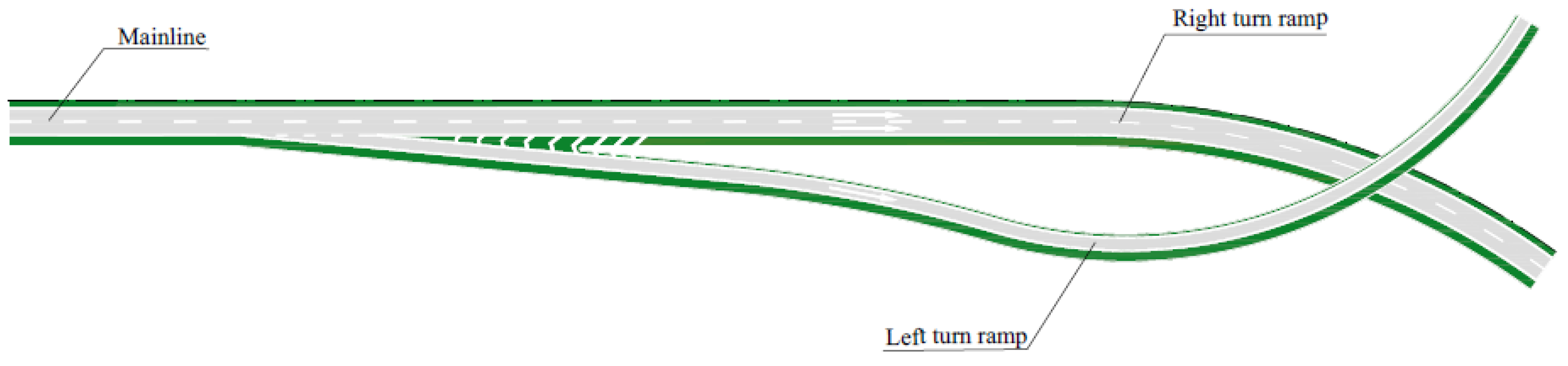
In the context of RTRL, drivers intending to make a left turn within the diversion area must effectively identify the right-side exit from the mainline in front of them to navigate the right diversion safely, as shown in Figure 13. Findings from driver simulation studies indicate that drivers encounter a more intricate scenario in path selection when facing the design of RTRL. Thus, ensuring an adequate decision sight distance within the right-turn ramp on the left diversion area holds particular significance.
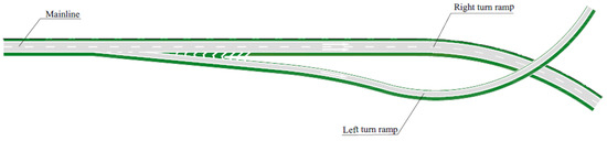
Figure 13.
The right-turn ramps to the left of the diversion area.
According to A Policy on Geometric Design of Highways and Streets (The Green Book), decision sight distance refers to the distance necessary for a driver to detect unexpected or challenging-to-perceive elements or conditions in a visually dense roadway environment. Notably, these values significantly exceed the values of the stopping sight distance. However, the policy lacks specifications regarding the decision sight distance values required for the exit of interchanges at different design speeds, and also does not provide a defined scope. On the other hand, the Intersections Guidelines of China outline the decision sight distance value, which needs to be met before the diversion nose end of the interchange. This guideline considers the diversion nose end as the endpoint of the decision sight distance. Nevertheless, the triangular area preceding the diversion nose typically comprises a solid line, prohibiting vehicles from crossing. Consequently, diverging vehicles are required to complete the decision and lane-change progress before reaching the triangle. Suppose the length of the triangle is part of the decision sight distance. In this case, it might inadvertently suggest allowing vehicles to breach the triangular marking to change lanes, thereby contravening traffic management regulations.
Binghong Pan [33] conducted an investigation and visual gaze point location analysis experiment and concluded that considering its supportive role in efficient vehicle diverging, the starting point of the taper of the deceleration lane is deemed the decision sight distance destination. Consequently, this study defines the decision sight distance range as starting from the driver’s perspective of the exit position up to the initiation of the downstream taper of the deceleration lane.
The decision sight distance model (Figure 14) was developed based on the most unfavorable driving conditions, where before the diversion area diverging vehicles were driving on the second outer lane. Therefore, the model proposes that the complete diversion behavior should include decision-making, queuing for gaps, and executing lane-changing stages, as shown in Equation (10).
where S denotes decision sight distance (m), denotes decision distance (m), represents queuing distance (m), and signifies execution of lane-change distance (m).
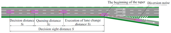
Figure 14.
Calculation model for decision sight distance.
4.2. Decision Distance S1
It is considered that the vehicle maintains a constant vehicle speed during the driver’s response to the sign, as determined in Equation (11):
where is the vehicle speed (km/h) in the decision process, which can be taken as the design vehicle speed of the mainline. denotes the decision time (s).
According to the Intersections Guidelines, ideal decision times of 2.5 s, 2.5 s, and 2.4 s are specified for design speeds of 120 km/h, 100 km/h, and 80 km/h, respectively. When drivers lack anticipation regarding driving decisions and must abruptly decide whether to exit from the mainline after suddenly discovering the exit, a longer decision time is required compared to situations where anticipation exists. The road environment’s complexity faced by drivers in RTRL differs from that of a traditional exit, necessitating a more extensive decision time for drivers. The length of the decision time is influenced by the complexity of the decision, notably the extent of the information involved in the decision-making process [32]. The correlation between the drivers’ decision time and information capacity without anticipation is elucidated in Equation (12):
where x signifies the information capacity. In conventional exit sections, drivers can continue straight or change lanes within 1-bit information capacity [32]. To ensure drivers promptly adapt to the RTRL and make a timely and accurate choice of the correct path, considering an information capacity of 2 bits, the calculation of tf takes 3.166 s, thus adopting a reaction time of 3.2 s.
4.3. Queuing Distance S2
Throughout the queuing phase, it is assumed that the driver maintains a constant vehicle speed within the current lane, awaiting an available gap in the target lane. The queuing distance S2 is calculated using Equation (13):
where denotes vehicle speed during the queuing process (km/h), derived from the mainline design speed and the diversion vehicle speed. Diversion vehicle speed is the vehicle speed in the curb lane of the mainline at the beginning cross-section of the deceleration lane taper while indicating the queuing time (s).
When the time headway of vehicles in the diversion area adheres to a 2-stage Erlang distribution, Equation (14) depicts the average count of vehicles n within non-insertable gaps and the average duration h for the occurrence of non-insertable gaps:
where tc is the minimum insertable gap critical value, which can be taken as 3.75 [33].
The calculated average queuing time for insertable gaps for lane-changing vehicles, denoted as tw, is determined by Equation (15):
where denotes the average rate of vehicles reaching the curb lane of the mainline per unit of time (pcu/s), , and represents the maximum service traffic volume of a single lane for the mainline (pcu/h/ln), the level of service is taken as the LOS-C.
4.4. Execution of Lane-Change Distance S3
Upon the emergence of an available gap within the curb lane of the mainline, vehicles initiate lane-changing maneuvers. Building upon the analysis, it becomes evident that the adapted hyperbolic tangent function lane-changing model more accurately captures the lane-changing patterns exhibited by vehicles navigating the interchange diversion area, particularly concerning the RTRL. At this stage, the mathematical representation of the vehicle’s lateral vehicle speed, lateral acceleration, and rate of change of lateral acceleration is encapsulated by Equation (16).
Considering passengers’ comfort throughout the vehicle’s lane-change maneuver, the lateral acceleration and its rate of change are required to conform to the constraints delineated in Equations (17) and (18).
Integrating the aforementioned equation, the expression for the length of the lane change is detailed in Equation (19) as follows:
where represents the maximum value of lateral acceleration (m/s2); signifies the maximum value of the emergency coefficient of lane changing; is the lateral displacement (m) during the lane-changing process, taking 3.75 m; symbolizes the vehicle speed (m/s) in the process of lane changing, takes the mainline diversion vehicle speed. denotes the maximum value of the rate of change of lateral acceleration (m/s3). Various countries have adopted distinct values within their road specifications. For instance, the United States prescribes 0.61 m/s3, West Germany designates 0.5 m/s3, while the United Kingdom typically utilizes 0.305 m/s3. In Japan, the range varies from 0.5 m/s3 to 0.75 m/s3, and in China, the usual range is 0.5 m/s3 to 0.6 m/s3, with the discretion exercised in actual application. By consolidating the findings from the aforementioned research, this paper computes the intermediate value of the provided range, adopting 0.6 m/s3 as the value .
The Green Book outlines the maximum permissible superelevation as either 8% or 10%, while the Intersections Guidelines specify that for design speeds exceeding 80 km/h, the superelevation should not exceed 3% and 4%, respectively. These specifications form the foundation for establishing both the general minimum radius value of the mainline curve and limit of the minimum radius value of the interchange. Thus, accounting for the most unfavorable scenario, the calculation of lateral acceleration utilizes 4% of the reverse superelevation by Equation (20), and the resultant value is considered as the maximum lateral acceleration:
where denotes the side friction factors, it is valued according to Technical Standard of Highway Engineering; represents cross slope; signifies gravitational constant, 9.8 m/s2.
The process parameters and calculation results for determining the decision sight distance of the exit within the right-turn ramp on the left at the interchange are tabulated in Table 5, utilizing the decision sight distance calculation model formula.
Table 5.
The parameters and recommended values for the decision sight distance calculation process.
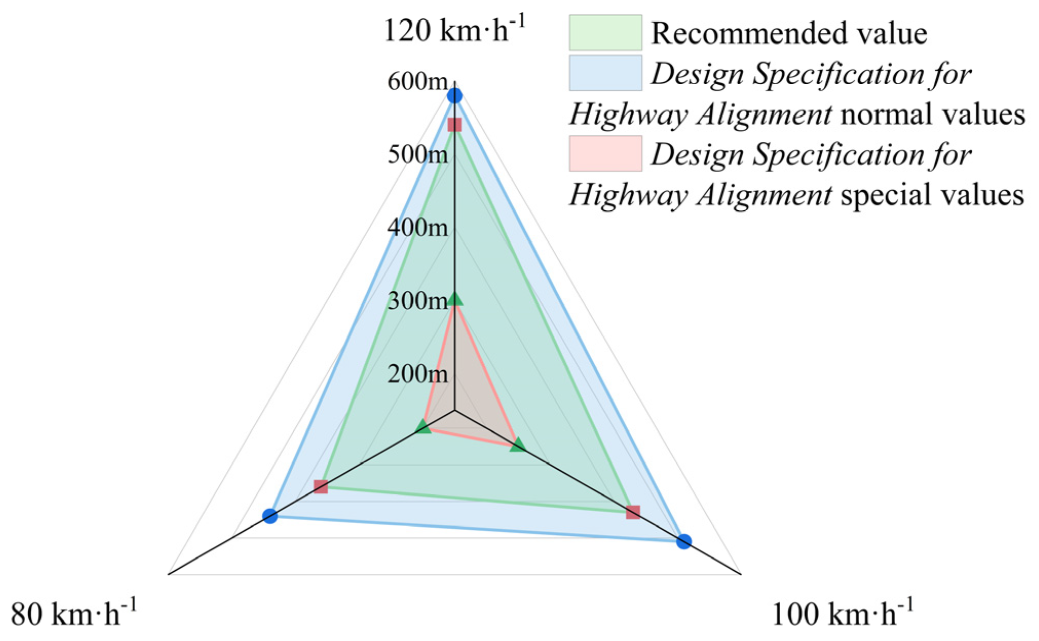
The Green Book does not specify an exact value for the decision sight distance. In contrast to the Design Specification for Highway Alignment, as depicted in Figure 15, it is evident that the specified sight distance values fall below the recommended values across all design vehicle speed levels. Given the unique nature of the right-turn ramp on the left, relying solely on these specified values for exit recognition of visual distance might pose challenges in meeting the visual distance requirements for drivers within the interchange exit section, potentially compromising diversion efficiency and safety. Therefore, it is necessary to consider augmenting the recognized visual distance based on an appropriate increase beyond the specified norms.
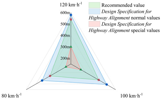
Figure 15.
The comparison of recommended value and standard value for decision sight distance.
In conclusion, a comprehensive investigation of drivers’ behavioral characteristics is imperative. This study aims to elucidate the rationale behind determining the identification of sight distance based on empirical data, with the overarching goal of enhancing the safety standards of interchanges.
5. Conclusions
This paper introduces a novel approach for determining the decision sight distance for right-turn ramps on the left within an interchange. The methodology encompasses several key steps: Firstly, utilizing UAV footage, this study captures and analyzes vehicle operational videos within the diversion area of two left-placed right-turn ramps. It delves into examining vehicle operating velocities, headway distances, and microscopic lane-change trajectory data. Secondly, a comprehensive driver behavior simulation test is conducted to explore various aspects such as vehicle speed fluctuations, visual characteristics, and psychological reactions within the right-turn ramp on the left section. Subsequently, the findings from the collected empirical data are applied to parameterize a decision sight distance calculation model, resulting in the recommended values for the decision sight distance in the context of the right-turn ramp on the left at freeway interchanges.
This study presents the following key findings:
- Utilizing UAV aerial photography combined with the YOLOv3 target detection algorithm, Kalman filtering, and the Frenet coordinate transformation method, microscopic lane-changing trajectory data is obtained. This data analysis sheds light on the travel speed, headway, and lane-changing behaviors within the left exit section of the right-turn ramp.
- Employing the modified hyperbolic tangent function lane-change trajectory model, Python calculations yield a 97.18% goodness of fit for the right lane change, affirming the accuracy of this model in depicting vehicle driving characteristics. Furthermore, the vehicle’s headway adheres to the 2-stage Erlang distribution, determining the waiting time.
- Simulated driving tests conducted using UC-win/Road simulation software, Forum8 driving simulation platform, and SMI ETGTM spectacle-type eye-tracking device analyze driver accuracy, workload, and traffic and visual behavior characteristics within the left-handed section of the right-turn on-ramp at the interchange.
- A formulated model for calculating the decision sight distance within the left-placed right-turn ramp section of the interchange is presented. This model segments the decision distance, queuing distance, and execution lane-changing distance, elucidating the underlying principles for calculating the decision sight distance. Sequential calibration of the relevant model parameters based on the measured data and driver behavior simulation experiments yields recommended decision sight distance values corresponding to different mainline design velocities.
- Chinese specified sight distance values appear smaller than the recommended value, raising concerns regarding the potential insufficiency of the decision sight distance when adopting the Route Specification’s special value due to the distinctive nature of the right-turn ramp left placement.
Due to space constraints, this paper primarily investigates traffic data at design velocities of 120 km/h and 100 km/h, limiting the investigation area and sample. Future research directions involve expanding the dataset to include 80 km/h traffic data, augmenting the sample sizes, and further exploring the traffic characteristics of trucks.
Author Contributions
Conceptualization, Z.F. and J.Z.; methodology, J.Z. and B.P.; validation, S.W. and B.P.; formal analysis, S.W.; investigation, H.Y. and J.Z.; resources, B.P. and J.Z.; data curation, S.W. and H.Y.; writing—original draft preparation, Z.F.; writing—review and editing, B.P. and J.Z.; visualization, H.Y.; supervision, B.P.; project administration, S.W.; funding acquisition, B.P. All authors have read and agreed to the published version of the manuscript.
Funding
This research was funded by the Scientific Research Program of CCCC First Highway Consultants Co., Ltd. (Study on Highway Parking Sight Distance No. KCJJ2022-23).
Institutional Review Board Statement
Not applicable.
Informed Consent Statement
Not applicable.
Data Availability Statement
The raw data supporting the conclusions of this article will be made available by the authors on request.
Conflicts of Interest
Authors Zhipeng Fu and Shangen Wu were employed by the company CCCC First Highway Consultants Co., Ltd. The authors declare that this study received funding from Scientific Research Program of CCCC First Highway Consultants Co., Ltd. The funder was not involved in the study design, collection, analysis, interpretation of data, the writing of this article or the decision to submit it for publication.
Abbreviations
| RTRL | right-turn ramps on the left |
| UAV | unmanned aerial vehicles |
| LCR | lane change to the right side |
References
- Wang, X.; Lin, R.; Ye, W.; Ma, Z. Are Expensive Expressways in China Attractive to Businesses? Evidence From the Location Selections of Manufacturing Enterprises. Transp. Res. Rec. J. Transp. Res. Board 2023, 2677, 567–578. [Google Scholar] [CrossRef]
- Abatan, A.; Savolainen, P.T. Safety Analysis of Interchange Functional Areas. Transp. Res. Rec. J. Transp. Res. Board 2018, 2672, 120–130. [Google Scholar] [CrossRef]
- Heddebaut, O.; Di Ciommo, F. City-hubs for smarter cities. The case of Lille “EuraFlandres” interchange. Eur. Transp. Res. Rev. 2017, 10, 10. [Google Scholar] [CrossRef]
- Wu, Z.Y.; Fu, Q. Research on Fiber Micro-Surfacing Mixture Design and Pavement Performance in Interchange’s Connections. In Proceedings of the 5th International Conference on Civil Engineering and Transportation, Guangzhou, China, 28–29 November 2015; pp. 167–174. [Google Scholar]
- Lan, C.J.; Li, J.; Chimba, E.D. Statistical Evaluation of Motorcycle Crash Injury Severities by Using Multinomial Models. In Proceedings of the Transportation Research Board of the National Academies, Washington, DC, USA, 22–26 June 2006. [Google Scholar]
- McCartt, A.T.; Northrup, V.S.; Retting, R.A. Types and characteristics of ramp-related motor vehicle crashes on urban interstate roadways in Northern Virginia. J. Saf. Res. 2004, 35, 107–114. [Google Scholar] [CrossRef]
- Hongchao, L.; Shisheng, L.; Zhongxiang, F.; Kun, W.; Yewei, L. Driving anger in China: A case study on professional drivers. Transp. Res. Part F Traffic Psychol. 2016, 42, 255–266. [Google Scholar]
- Xu, S.X.; Liu, T.L.; Huang, H.J.; Liu, R. Mode choice and railway subsidy in a congested monocentric city with endogenous population distribution. Transp. Res. Part A Policy Pract. 2018, 116, 413–433. [Google Scholar] [CrossRef]
- Chen, F.; Chen, S. Injury severities of truck drivers in single- and multi-vehicle accidents on rural highways. Accid. Anal. Prev. 2011, 43, 1677–1688. [Google Scholar] [CrossRef]
- Chen, F.; Peng, H.; Ma, X.; Liang, J.; Hao, W.; Pan, X. Examining the safety of trucks under crosswind at bridge-tunnel section: A driving simulator study. Tunn. Undergr. Space Technol. 2019, 92, 103034. [Google Scholar] [CrossRef]
- Feng, Z.; Yang, M.; Ma, C.; Kang, J.; Yewei, L.; Huang, W.; Huang, Z.; Zhan, J.; Zhou, M. Driving anger and its relationships with type A behavior patterns and trait anger: Differences between professional and non-professional drivers. PLoS ONE 2017, 12, e0189793. [Google Scholar] [CrossRef]
- Guerrieri, M.; Mauro, R.; Tollazzi, T.J.T.E.P.A.S. Turbo-Roundabout: Case Study of Driver Behavior and Kinematic Parameters of Light and Heavy Vehicles. J. Transp. Eng. Part A Syst. 2019, 145. [Google Scholar] [CrossRef]
- Wang, C.; Lu, L.; Lu, J.; Wang, T. Selection for optimal exit ramp type on Florida’s freeways based on operational analysis. Adv. Mech. Eng. 2016, 8, 1–8. [Google Scholar] [CrossRef]
- Kayes, M.I.; Sandt, A.; Al-Deek, H.; Uddin, N.; Rogers, J.H.; Carrick, G. Modeling Wrong-Way Driving Entries at Limited Access Facility Exit Ramps in Florida. Transp. Res. Rec. J. Transp. Res. Board 2019, 2673, 567–576. [Google Scholar] [CrossRef]
- Atiquzzaman, M.; Zhou, H. Modeling the Risk of Wrong-Way Driving Entry at the Exit Ramp Terminals of Full Diamond Interchanges. Transp. Res. Rec. J. Transp. Res. Board 2018, 2672, 35–47. [Google Scholar] [CrossRef]
- Wu, P.; Meng, X.; Song, L. Identification and spatiotemporal evolution analysis of high-risk crash spots in urban roads at the microzone-level: Using the space-time cube method. J. Transp. Saf. Secur. 2022, 14, 1510–1530. [Google Scholar] [CrossRef]
- Wang, T.; Wang, C.; Qian, Z. Development of a new conflict-based safety metric for freeway exit ramps. Adv. Mech. Eng. 2017, 9, 1687814017723286. [Google Scholar] [CrossRef]
- Li, Z.; Wang, W.; Liu, P.; Bai, L.; Du, M. Analysis of Crash Risks by Collision Type at Freeway Diverge Area Using Multivariate Modeling Technique. J. Transp. Eng. 2015, 141, 04015002. [Google Scholar] [CrossRef]
- Chen, H.; Liu, P.; Lu, J.J.; Behzadi, B.J.A.A. Evaluating the safety impacts of the number and arrangement of lanes on freeway exit ramps. Accid. Anal. Prev. 2009, 41, 543–551. [Google Scholar] [CrossRef]
- Zahabi, M.; Machado, P.; Lau, M.Y.; Deng, Y.; Pankok, C.; Hummer, J.; Rasdorf, W.; Kaber, D.B. Driver performance and attention allocation in use of logo signs on freeway exit ramps—ScienceDirect. Appl. Ergon. 2017, 65, 70–80. [Google Scholar] [CrossRef]
- Bassan, S. Decision Sight Distance Review and Evaluation. Traffic Eng. Control. 2011, 52, 23–26. [Google Scholar]
- Ho, G.; Rozental, J.J.; Majstorović, S. Decision Sight Distance for Freeway Exit Ramps—A Road Safety Perspective. Eng. Environ. Sci. 2016. [Google Scholar]
- Liu, B.S.; Tseng, H.Y.; Pan, C.H.; Chia, T.C. Association of vehicle types and traffic conditions on driving speed at the freeway exit ramp. In Proceedings of the 38th International Conference on Computers & Industrial Engineering, Beijing, China, 31 October–2 November 2008. [Google Scholar]
- Lyu, N.; Cao, Y.; Wu, C.; Xu, J.; Xie, L. The effect of gender, occupation and experience on behavior while driving on a freeway deceleration lane based on field operational test data. Accid. Anal. Prev. 2018, 121, 82–93. [Google Scholar] [CrossRef] [PubMed]
- Calvi, A.; Bella, F.; D’Amico, F. Evaluating the effects of the number of exit lanes on the diverging driver performance. J. Transp. Saf. Secur. 2018, 10, 105–123. [Google Scholar] [CrossRef]
- Lasky, T.A.; Yen, K.; Ravani, B. Evaluating Wrong-Way Driving Incidents at Highway Exit Ramps and the Effect of Mitigation. J. Transp. Eng. Part A Syst. 2021, 147, 04021086. [Google Scholar] [CrossRef]
- Wei, M.; Teng, D.; Wu, S. Trajectory planning and optimization algorithm for automated driving based on Frenet coordinate system. Control. Decis. 2021, 36, 815–824. [Google Scholar]
- Wu, S.B.; Zou, Y.J.; Wu, L.T.; Zhang, Y. Application of Bayesian model averaging for modeling time headway distribution. Phys. A—Stat. Mech. Its Appl. 2023, 620, 128747. [Google Scholar] [CrossRef]
- Pan, B.; Wang, C.; Wang, Q.; Ma, Z.; Xie, Z. A Study of Length of Auxiliary Lanes for Two-Lane Expressway Exits Based on Microscopic Lane Change. J. Tongji Univ. Nat. Sci. 2022, 50, 1647–1657. [Google Scholar]
- Li, L.; Liu, Y.; Wang, J.; Deng, W.; Oh, H. Human dynamics based driver model for autonomous car. Intell. Transp. Syst. 2016, 10, 545–554. [Google Scholar] [CrossRef]
- Piranveyseh, P.; Kazemi, R.; Soltanzadeh, A.; Smith, A. A field study of mental workload: Conventional bus drivers versus bus rapid transit drivers. Ergonomics 2022, 65, 804–814. [Google Scholar] [CrossRef] [PubMed]
- Evans, J.L.; Elefteriadou, L.; Gautam, N. Probability of breakdown at freeway merges using Markov chains. Transp. Res. Part B Methodol. 2001, 35, 237–254. [Google Scholar] [CrossRef]
- Pan, B.; Zhou, X.; Zhou, T.; Zhao, Y.; Yang, C. Decision Sight Distance Calculation Model of Expressway Interchange Exit. J. Tongji Univ. Nat. Sci. 2020, 48, 1312. [Google Scholar]


Disclaimer/Publisher’s Note: The statements, opinions and data contained in all publications are solely those of the individual author(s) and contributor(s) and not of MDPI and/or the editor(s). MDPI and/or the editor(s) disclaim responsibility for any injury to people or property resulting from any ideas, methods, instructions or products referred to in the content. |
© 2024 by the authors. Licensee MDPI, Basel, Switzerland. This article is an open access article distributed under the terms and conditions of the Creative Commons Attribution (CC BY) license (https://creativecommons.org/licenses/by/4.0/).