X-ray Pulsar-Based Navigation Using Pulse Phase Delay between Spacecraft and Verification with Real Data

Abstract

Pulsars are neutron stars with high rotation speeds and have extraordinary long-term rotational stability. X-ray pulsar-based navigation (XNAV) is a navigation method that estimates the position and velocity of a spacecraft using the X-ray radiation from pulsars. Flight experiments on Insight-Hard X-ray Modulation Telescope (Insight-HXMT) and Neutron Star Interior Composition Explorer (NICER) have successfully verified the feasibility of using XNAV for a single spacecraft. For spacecraft in formation, a pulsar-based navigation method that uses the pulse phase delay between spacecraft is derived. Moreover, a direct estimation method for pulse phase delay, which is independent from the pulsar template, is proposed. The proposed method is verified with simulation data of the Crab pulsar and real data of the same pulsar obtained from Insight-HXMT and NICER.

1. Introduction

With the development of aerospace technology, on-orbit spacecraft missions have become more complex [1]. Formation spacecraft have the advantages of low system cost and high flexibility [2,3]. Compared to a single spacecraft, spacecraft formation flying is more flexible for complex space missions [4]. Thus, spacecraft formation flying has attracted a lot of attention [5,6]. Furthermore, navigation services are important for spacecraft formation flying missions [7].

XNAV is a developing autonomous navigation method providing navigation services for Earth-orbit and deep-space spacecraft [8,9]. The basic idea of the XNAV for a single spacecraft is similar with that of the Global Navigation Satellite System. A spacecraft estimates its position and velocity using received photons from different pulsars [10]. Since its introduction in 1981, a significant growth in the navigation algorithm for XNAV has occurred in the past four decades [11,12]. In addition, some flight experiments, such as NICER and Insight-HXMT, were performed [13,14,15,16].

Aside from providing navigation service for a single spacecraft, XNAV can also be used for spacecraft in formation [17,18,19]. In [17], Xiong proposed the use of time difference of arrival (TDOA) measurements from pulsars and pseudo-range observations from inter-satellite links to determine the position of a satellite in the constellation. In [18], Zhang proposed using TDOA, phase increment, the baseline of double satellites, and the plane formed by three satellites for spacecraft formation navigation. In [19], Emadzadeh proposed the use of pulse delay between two spacecraft to estimate the relative position and studied the effect of velocity errors on position estimation. However, in [19], the pulse delay is calculated after pulse phases of spacecraft are estimated, respectively. This can lead to unnecessary redundant calculations. Moreover, in [19], the pulse phase of spacecraft is estimated using the template of pulsar and empirical profiles recovered form pulsar photons. However, this can affect the estimation performance of the pulse phase based on the accuracy of the template. In [17,18,19], the proposed methods were only verified through simulation.

In this paper, we first described a pulse phase estimation method and the measurement model of XNAV for a single spacecraft. Then, taking the formation of two spacecraft as an example, a pulsar-based navigation method is used to derive the pulse phase delay between spacecraft. To improve computational efficiency and eliminate dependence on the template of pulsars, a direct estimation method for pulse delay without using a template is proposed. The proposed method is verified with simulation data of the Crab pulsar and real data of the Crab pulsar derived from NICER and Insight-HXMT. For convenience, we only consider the Romer delay and Shapiro delay when determining the transform photon arrival time from spacecraft to solar system barycenter (SSB). To provide an accurate navigation service for spacecraft near gravitational sources, an accurate transform model should be considered in further studies [20].

The remainder of the paper is organized as follows: The related method of XNAV for a single spacecraft is shown in Section 2; Section 3 derives a pulsar-based navigation method using the pulse phase delay between spacecraft, and a direct estimation method is proposed for pulse phase delay. In Section 4, the simulation data of the Crab pulsar and the real data of the Crab pulsar derived from NICER and Insight-HXMT are used to verify the proposed method. The conclusions are presented in Section 5.

2. Related Method of XNAV for Single Spacecraft

2.1. Measurement Model

The measurement of pulsar-based navigation is the pulse phase. The pulse phase at $t_i$ can be expressed as [16] follows:

$$\varphi (t_i)=F_0[g(t_i)-T_0]+{\displaystyle \frac{F_1}{2}}[g(t_i)-T_0{]}^2,$$

(1)

where $F_0$ and $F_1$ are the frequency of the pulsar and the time derivative of the frequency at $T_0$, respectively, and $F_0$ and $F_1$ can be found in the public pulsar ephemeris [21]. In addition, $g\left(t_i\right)$ can be described by [20,22] the following:

$$g(t_i)=t_i+{\displaystyle \frac{\mathit{n}\cdot ({\mathit{r}}_i+{\mathit{r}}_{E,i})}{c}}+{\sum }_{k=1}^K{\displaystyle \frac{2{\mu }_k}{c^3}}\mathit{ln}|\mathit{n}\cdot {\mathit{r}}_{k,i}+‖{\mathit{r}}_{k,i}‖|,$$

(2)

where c is the speed of light, ${\mathit{r}}_i$ is position vector of the spacecraft relative to the Earth at $t_i$, n is the direction vector of the pulsar, ${\mathit{r}}_{E,i}$ is the position vector of Earth relative to the SSB at $t_i$, ${\mathit{r}}_{k,i}$ is the position of the spacecraft relative to the kth celestial body(unit m), ${\mu }_k$ is the gravitational coefficient of the kth celestial body, and ‖ ‖ is the magnitude of the vector. The second and third terms on the right side of Equation (2) are the Romer delay and the Shapiro delay, respectively. The Romer delay represents a vacuum delay between the spacecraft and the SSB, while the Shapiro delay represents a time delay caused by the pulse passing through curved space–time.

Assuming that ${\mathit{x}}_i=\mathit{x}\left(t_i\right)=[{\mathit{r}}_i,{\mathit{v}}_i]$, $y_i=\varphi \left(t_i\right)={\varphi }_i$, and $h({\mathit{x}}^i)=F_0[g(t_i)-T_0]+{\displaystyle \frac{F_1}{2}}[g(t_i)-T_0{]}^2$, ${\mathit{v}}_i$ is the velocity of the spacecraft relative to the Earth at $t_i$. Thus, Equation (1) can be rewritten as [16] follows:

$$y_i=h\left({\mathit{x}}_i\right).$$

(3)

2.2. Pulse Phase Estimation Method

The pulsar is very weak such that a spacecraft can only receive a series of events rather than a continuous pulsed signal. Thus, a spacecraft must estimate the pulse phase from received events [23].

Let us assume a spacecraft observes a pulsar from $t_i$ to $t_{i+1}$, i = 1, 2, …I and receives N events $\{{\tau }_j{\}}_{j=1}^N$. At first, $\{{\tau }_j{\}}_{j=1}^N$ should be corrected to SSB by (2); thus, we have 16:

$${\tau }_{j,SSB}=g\left({\tau }_j\right).$$

(4)

Therefore, the pulse phase at ${\tau }_{j,SSB}$ is expressed as

$$\varphi ({\tau }_{j,SSB})={\varphi }_i+F_i[g({\tau }_j)-g(t_i)]+{\displaystyle \frac{1}{2}}{\dot{F}}_i[g\left({\tau }_j\right)-g\left(t_i\right){]}^2,$$

(5)

where ${\varphi }_i=\varphi \left(t_i\right)$ is the pulse phase at $g\left(t_i\right)$, $F_i$ is the frequency at $g\left(t_i\right)$, and ${\dot{F}}_i$ is the time derivative of the frequency at $g\left(t_i\right)$, respectively.

However, the true position of the spacecraft, $\mathit{r}\left({\tau }_j\right)$ in (2), is inaccessible in an autonomous navigation task. $\mathit{r}\left({\tau }_j\right)$ is expressed as $\mathit{r}\left({\tau }_j\right)=\tilde{\mathit{r}}\left({\tau }_j\right)+\delta \mathit{r}\left({\tau }_j\right)$ to estimate the pulse phase, where $\tilde{\mathit{r}}\left({\tau }_j\right)$ is the predicted position of the spacecraft and $\delta \mathit{r}\left({\tau }_j\right)$ is the error of $\tilde{\mathit{r}}\left({\tau }_j\right)$. Moreover, $\delta \mathit{r}\left({\tau }_j\right)$ can be derived as functions of $\delta \mathit{v}\left({\tau }_i\right)$ and $\delta \mathit{r}\left({\tau }_i\right)$ [24,25,26]:

$$\delta \mathit{r}\left({\tau }_j\right)={\mathit{\Phi }}_{rr}({\tau }_j,{\tau }_i)\delta \mathit{r}\left({\tau }_i\right)+{\mathit{\Phi }}_{rv}({\tau }_j,{\tau }_i)\delta \mathit{v}\left({\tau }_i\right),$$

(6)

where $\delta \mathit{v}\left({\tau }_i\right)$ is the error of the predicted velocity of the spacecraft $\tilde{\mathit{v}}\left({\tau }_j\right).\mathrm{I}\mathrm{n}\mathrm{a}\mathrm{d}\mathrm{d}\mathrm{i}\mathrm{t}\mathrm{i}\mathrm{o}\mathrm{n},{\mathit{\Phi }}_{rr}({\tau }_j,{\tau }_i)$ and ${\mathit{\Phi }}_{rv}\left({\tau }_j,{\tau }_i\right)$ can be expressed as [24,25] follows:

$$\begin{array}{c}{\mathit{\Phi }}_{rr}({\tau }_j,{\tau }_i)=I_{3\times 3}+{\sum }_{m=1}^{\infty }{\displaystyle \frac{1}{m!}}{\mathit{\phi }}_m{\left({\tau }_j-{\tau }_i\right)}^m\\ {\mathit{\Phi }}_{rv}({\tau }_j,{\tau }_i)={\sum }_{m=1}^{\infty }{\displaystyle \frac{1}{m!}}{\mathit{\gamma }}_m{\left({\tau }_j-{\tau }_i\right)}^m\end{array},$$

(7)

where ${\mathit{\phi }}_m$ and ${\mathit{\gamma }}_m$ are constant matrixes that can be calculated using analytical, numerical, or finite difference techniques [26].

Therefore, (5) can be rewritten as [27]:

$$\varphi \left({\tau }_{j,SSB}\right)={\varphi }_i+F_i^{Doppler}\left({\tau }_j-t_i\right)+\tilde{\varphi }\left({\tau }_{j,SSB}\right),$$

(8)

where

$$\tilde{\varphi }({\tau }_{j,SSB})=F_i[\tilde{g}({\tau }_j)-\tilde{g}(t_i)]+{\displaystyle \frac{1}{2}}{\dot{F}}_i[\tilde{g}\left({\tau }_j\right)-\tilde{g}\left(t_i\right){]}^2,$$

(9)

$$\tilde{g}(t_i)=t_i+{\displaystyle \frac{n\cdot \left(\tilde{\mathit{r}}\left(t_i\right)+{\mathit{r}}_E\left(t_i\right)\right)}{c}}+{\sum }_{k=1}^K{\displaystyle \frac{2{\mu }_k}{c^3}}\mathit{ln}|n\cdot {\tilde{\mathit{r}}}_k(t_i)+‖{\tilde{\mathit{r}}}_k\left(t_i\right)‖|,$$

(10)

$$F_i^{orbit}=F_i[{\mathit{G}}_i{\mathit{\phi }}_1\delta \mathit{r}(t_i)+{\mathit{G}}_i{\mathit{\gamma }}_1\delta \mathit{v}(t_i)],$$

(11)

$$\begin{array}{cc}\hfill {\mathit{G}}_i& ={{\displaystyle \frac{\partial g(t_i)}{\partial \mathit{r}(t_i)}}|}_{\mathit{r}(t_i)= \tilde{\mathit{r}}(t_i)}\hfill \\ & ={\displaystyle \frac{1}{c}}\mathit{n}+2{\displaystyle \sum _k\frac{{\mu }_k}{c^3}}{\displaystyle \frac{n\Vert { \tilde{\mathit{r}}}_k(t_i)\Vert +{ \tilde{\mathit{r}}}_k(t_i)}{\left|\mathit{n}·{ \tilde{\mathit{r}}}_k(t_i)+\Vert { \tilde{\mathit{r}}}_k(t_i)\Vert \right|\Vert { \tilde{\mathit{r}}}_k(t_i)\Vert }}.\hfill \end{array}$$

(12)

In the equations above, $\tilde{\varphi }\left({\tau }_{j,SSB}\right)$ and $\tilde{g}\left(t_i\right)$ are the pulse phase and photon arrival time calculated by $\tilde{\mathit{r}}\left(t_i\right)$, respectively. Applying (8) to every event $\{{\tau }_j{\}}_{j=1}^N$, we have $\left\{\varphi \right({\tau }_{j,SSB}){\}}_{j=1}^N$. Thus, we have to estimate ${\varphi }_0^i$ and $F_i^{orbit}$ from $\left\{\varphi \right({\tau }_{j,SSB}){\}}_{j=1}^N$.

Here, $F_i^{orbit}$ and ${\varphi }_0^i$ can be estimated using the epoch folding method. The observation period is assumed to consist of $M$ pulsar periods in the epoch folding method. The period can be divided into $M_b$ equal-length bins. The length of each bin is assumed as $t_b$, and $c_l^m$ is the number of detected photons in the $l-th$ bin of the $m-th$ period. Therefore, the empirical profile can be recovered. Here, we define the empirical profile function at ${\phi }_l$ as [19] the following:

$${\lambda }_{EF}\left({\phi }_l;F_i^{orbit}\right)={\displaystyle \frac{1}{M{t}_b}}{\sum }_{m=1}^M{c}_l^m\left({\phi }_l;F_i^{orbit}\right),$$

(13)

where ${\phi }_l$ is the pulse phase at the middle of $l-th$ bin.

We adopt the Chi-squared test to calculate the statistical characteristics of the empirical profile as follows [28]:

$${\chi }^2={\sum }_{l=1}^{M_b}{\displaystyle \frac{(C_l-\overline{C}{)}^2}{\overline{C}}},$$

(14)

where

$$C_l={\sum }_{m=1}^M{c}_l^m({\phi }_l;F_i^{orbit}),$$

(15)

$$\overline{C}={\displaystyle \frac{{\sum }_{m=1}^M{\sum }_{l=1}^{M_b}{c}_l^m({\phi }_l;F_i^{orbit})}{M_b}},$$

(16)

Using Equations (14)–(16), ${\overline{\upsilon }}_1$ can be estimated with

$${\hat{F}}_i^{orbit}=\mathit{arg}\underset{F_i^{Doppler}}{max}{\chi }^2.$$

(17)

$\mathrm{I}\mathrm{n}\mathrm{a}\mathrm{d}\mathrm{d}\mathrm{i}\mathrm{t}\mathrm{i}\mathrm{o}\mathrm{n}, {\varphi }_i$ can be estimated by solving a nonlinear least squares estimation problem [19]:

$$J\left({\varphi }_i\right)={\sum }_{l=0}^{M_b}{\left[{\lambda }_{EF}({\phi }_l;{\hat{F}}_i^{orbit})-{\lambda }_{Te}({\phi }_l)\right]}^2,$$

(18)

where ${\lambda }_{Te}$ is the template of the pulsar.

At the same time, ${\varphi }_i$ can be estimated with

$${\hat{\varphi }}_i=\underset{{\varphi }_i\in \left[0,1\right)}{\arg \min J\left({\varphi }_i\right)}.$$

(19)

3. XNAV for Spacecraft in Formation

3.1. Measurement Model

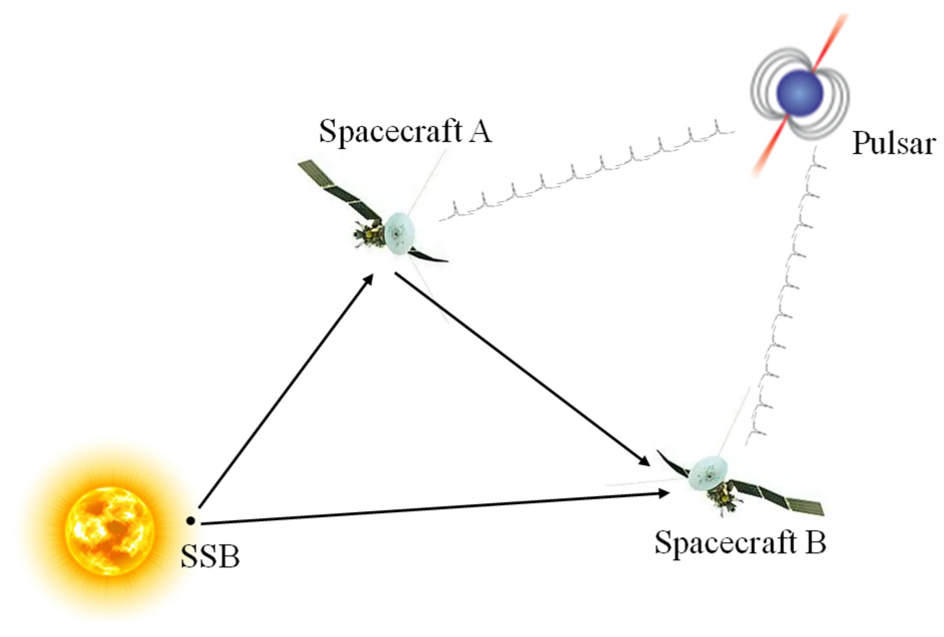
The diagram of XNAV for spacecraft in formation is shown in Figure 1. Assume that spacecraft A and spacecraft B observe the same pulsar; thus, according to (1), the pulse phases are given by

$${\varphi }_i^A={\varphi }_A(t_i)=F_0[g^A(t_i)-T_0]+{\displaystyle \frac{F_1}{2}}[g^A(t_i)-T_0{]}^2,$$

(20)

$${\varphi }_i^B={\varphi }_B(t_i)=F_0[g^B(t_i)-T_0]+{\displaystyle \frac{F_1}{2}}[g^B(t_i)-T_0{]}^2,$$

(21)

where

$$g^A(t_i)=t_i+{\displaystyle \frac{\mathit{n}\cdot ({\mathit{r}}_i^A+{\mathit{r}}_{E,i})}{c}}+{\sum }_{k=1}^K{\displaystyle \frac{2{\mu }_k}{c^3}}\mathit{ln}|\mathit{n}\cdot {\mathit{r}}_{k,i}^A+‖{\mathit{r}}_{k,i}^A‖|,$$

(22)

$$g^B(t_i)=t_i+{\displaystyle \frac{\mathit{n}\cdot ({\mathit{r}}_i^B+{\mathit{r}}_{E,i})}{c}}+{\sum }_{k=1}^K{\displaystyle \frac{2{\mu }_k}{c^3}}\mathit{ln}|\mathit{n}\cdot {\mathit{r}}_{k,i}^B+‖{\mathit{r}}_{k,i}^B‖|,$$

(23)

where ${\mathit{r}}_i^A$ is the position of spacecraft A relative to the Earth at $t_i$ $\mathrm{and}{\mathit{r}}_i^B$ is the position of spacecraft B relative to the Earth at $t_i$. Given that the distance between the two spacecraft is far less than the distances between the celestial bodies and the spacecraft, we assume that ${\mathit{r}}_{k,i}^A\approx {\mathit{r}}_{k,i}^B$, and we denote it as ${\mathit{r}}_{k,i}$.

Figure 1. Diagram of XNAV for spacecraft in formation.

We use pulse phase delay between spacecraft A and spacecraft B as a measurement:

$$\mathsf{\Delta }{\varphi }_i^{A,B}={\varphi }_i^A-{\varphi }_i^B$$

(24)

Substituting (20) and (21) into (24), we have

$$\mathsf{\Delta }{\varphi }_i^{A,B}=\frac{\mathit{n}\cdot ({\mathit{r}}_i^A-{\mathit{r}}_i^B)}{c}·[F_0+F_1·(t_i+\frac{\mathit{n}\cdot ({\mathit{r}}_i^A+{\mathit{r}}_{E,i})}{c}+{\displaystyle \sum _{k=1}^K\frac{2{\mu }_k}{c^3}}\ln |\mathit{n}\cdot {\mathit{r}}_{k,i}+\Vert {\mathit{r}}_{k,i}\Vert |-T_0)-\frac{F_1}{2}·\frac{\mathit{n}\cdot ({\mathit{r}}_i^A-{\mathit{r}}_i^B)}{c})].$$

(25)

Since c is about 3 × 10⁸ m/s, $F_1$ is smaller than 10⁻¹⁰ HZ/s for most pulsars. Assume that the distance between spacecraft A and B is shorter than 100 km. Therefore, ${\displaystyle \frac{F_1}{2}}{\displaystyle \frac{\mathit{n}\cdot ({\mathit{r}}_i^A-{\mathit{r}}_i^B)}{c}}$ is close to 0, and we have

$$\mathsf{\Delta }{\varphi }_i^{A,B}=\frac{\mathit{n}\cdot ({\mathit{r}}_i^A-{\mathit{r}}_i^B)}{c}·[F_0+F_1·(t_i+\frac{\mathit{n}\cdot ({\mathit{r}}_i^A+{\mathit{r}}_{E,i})}{c}+{\displaystyle \sum _{k=1}^K\frac{2{\mu }_k}{c^3}}\ln |\mathit{n}\cdot {\mathit{r}}_{k,i}+\Vert {\mathit{r}}_{k,i}\Vert |-T_0)].$$

(26)

We also define $F_i^{A,B}$ as follows:

$$F_i^{A,B}=F_0+F_1·(t_i+\frac{\mathit{n}\cdot ({\mathit{r}}_i^A+{\mathit{r}}_{E,i})}{c}+{\displaystyle \sum _{k=1}^K\frac{2{\mu }_k}{c^3}}\ln |\mathit{n}\cdot {\mathit{r}}_{k,i}+\Vert {\mathit{r}}_{k,i}\Vert |-T_0).$$

(27)

Substituting (27) into (25), we have

$$\mathsf{\Delta }{\varphi }_i^{A,B}=F_i^{A,B}{\displaystyle \frac{\mathit{n}\cdot \left({\mathit{r}}_i^A-{\mathit{r}}_i^B\right).}{c}}$$

(28)

Based on Equation (28), the difference in pulse phases of spacecraft A and spacecraft B reflects their distance in the direction of the pulsar. Assuming that $\mathsf{\Delta }{\mathit{x}}_i^{A,B}={\mathit{x}}_A(t_i)-{\mathit{x}}_B(t_i)$, $y_{i,AB}=\mathsf{\Delta }{\varphi }_i^{A,B}$ and $h_{A,B}(\mathsf{\Delta }{\mathit{x}}_i^{A,B})=F_i^{A,B}{\displaystyle \frac{\mathit{n}\cdot ({\mathit{r}}_i^A-{\mathit{r}}_i^B)}{c}}$, then Equation (28) can be rewritten as a standard measurement model of

$$y_{i,AB}=h_{A,B}\left(\mathsf{\Delta }{\mathit{x}}_i^{A,B}\right).$$

(29)

3.2. Pulse Phase Delay Estimation

In this section, we explain how the pulse phase delay can be abstained. Assume that spacecraft A and spacecraft B observe the same pulsar from $t_i$ to $t_{i+1}$, i = 1, 2,…I and receives $\{{\tau }_j^A{\}}_{j=1}^{N_A}$ and $\{{\tau }_j^B{\}}_{j=1}^{N_B}$, respectively. Applying (8) to $\{{\tau }_j^A{\}}_{j=1}^{N_A}$ and $\{{\tau }_j^B{\}}_{j=1}^{N_B}$, we have $\left\{\varphi \right({\tau }_{j,SSB}^A){\}}_{j=1}^N$ and $\left\{\varphi \right({\tau }_{j,SSB}^B){\}}_{j=1}^N$, where

$$\varphi \left({\tau }_{j,SSB}^A\right)={\varphi }_i^A+F_i^{orbit,A}({\tau }_j-t_i)+\tilde{\varphi }\left({\tau }_{j,SSB}^A\right),$$

(30)

$$\varphi \left({\tau }_{j,SSB}^B\right)={\varphi }_i^B+F_i^{orbit,B}\left({\tau }_j-t_i\right)+\tilde{\varphi }\left({\tau }_{j,SSB}^B\right).$$

(31)

As shown in Section 2.2, $F_i^{orbit,A}$ and $F_i^{orbit,B}$ can be estimated by (17). In Equation (19), ${\varphi }_i^A$ and ${\varphi }_i^B$ can be estimated by (18), and $\mathsf{\Delta }{\varphi }_i^{A,B}$ can be calculated by (24). However, when estimating ${\varphi }_i^A$ and ${\varphi }_i^B$, respectively, we have to solve the optimization problem shown in (18) twice, and the template is indispensable. To improve computational efficiency and eliminate dependence on the template, we proposed a direct estimation method for $\mathsf{\Delta }{\varphi }_i^{A,B}$.

Similar to (19), we define the cost function for estimating $\mathsf{\Delta }{\varphi }_i^{A,B}$ as follows:

$$J\left(\mathsf{\Delta }{\varphi }_i^{A,B}\right)={\sum }_{l=0}^{M_b}{\left[{\lambda }_{EF}^A({\phi }_l;{\hat{F}}_I^{\mathit{orbit},A})-{\lambda }_{EF}^B({\phi }_l;{\hat{F}}_I^{\mathit{orbit},B})\right]}^2.$$

(32)

Therefore, $\mathsf{\Delta }{\varphi }_i^{A,B}$ can be estimated by

$$\mathsf{\Delta }{\hat{\varphi }}_i^{A,B}=\underset{\mathsf{\Delta }{\varphi }_i^{A,B}\in \left[0,1\right)}{\arg \min J\left(\mathsf{\Delta }{\varphi }_i^{A,B}\right)}.$$

(33)

As shown in (32) and (33), $\mathsf{\Delta }{\varphi }_i^{A,B}$ can be estimated by solving (33) once and is independent from the template of pulsars.

3.3. Procedure of Pulsar-Based Navigation Using Pulse Phase Delay

In this section, we discuss the procedure of pulsar-based navigation using pulse phase delay between two spacecraft. We assume that the true position and velocity of spacecraft A is known, and the position and velocity of spacecraft B can be estimated by measuring pulse phase delay between spacecraft A and B. By measuring $\mathsf{\Delta }{\varphi }_i^{A,B}$, we can obtain the distance of the direction of the pulsar between spacecraft A and spacecraft B. Using one measurement, we can determine a ring of coordinate triples for spacecraft B. Moreover, given that the dynamic model of spacecraft B can be modeled in advance, we use an unscented Kalman filter (UKF) to estimate the state of spacecraft B using the measurement and dynamic model. The procedure of pulsar-based navigation using pulse phase delay is shown in Algorithm 1. At first, we apply (30) and (31) to $\{{\tau }_j^A{\}}_{j=1}^{N_A}$ and $\{{\tau }_j^B{\}}_{j=1}^{N_B}$ and obtain $\left\{\varphi \right({\tau }_{j,SSB}^A){\}}_{j=1}^N$ and $\left\{\varphi \right({\tau }_{j,SSB}^B){\}}_{j=1}^N$, respectively. Then, we estimate ${\hat{F}}_i^{orbit,A}$, ${\hat{F}}_i^{orbit,B}$ by (17) and estimate $\mathsf{\Delta }{\varphi }_i^{A,B}$ by (33). The state of spacecraft B is then estimated using UKF.

Algorithm 1. Procedure of pulsar-based navigation using pulse phase delay

Input: ${\mathbf{x}}_A\left(t_i\right)$, $\{{\tau }_j^A{\}}_{j=1}^{N_A}$, $\{{\tau }_j^B{\}}_{j=1}^{N_B}$ i = 1,2,…I 1. Initialization: Set initial state guess ${\tilde{\mathbf{x}}}_B\left(t_1\right)$.

2. for i = 1, 2,…I do

3.          $\mathsf{\Delta }{\tilde{\mathbf{x}}}_i^{A,B}={\mathbf{x}}_A(t_i)-{\tilde{\mathbf{x}}}_B(t_i)$ 4.        Predict the state of spacecraft B at $\{{\tau }_j^B{\}}_{j=1}^{N_B}$ by propagating ${\tilde{\mathbf{x}}}_B\left(t_i\right).$ 5.        Apply (30) and (31) to $\{{\tau }_j^A{\}}_{j=1}^{N_A}$ and $\{{\tau }_j^B{\}}_{j=1}^{N_B}$. 6.        Estimate ${\hat{F}}_i^{orbit,A}$ and ${\hat{F}}_i^{orbit,B}$ by (17). 7.        Recover empirical profile ${\lambda }_{EF}^A$ and ${\lambda }_{EF}^B$ by ${\hat{F}}_i^{orbit,A}$ and ${\hat{F}}_i^{orbit,B}$, respectively. 8.        Calculate $y_{i,AB}$ by (28) and (33). 9.        Estimate ${\hat{\mathbf{x}}}_B\left(t_i\right)$ by UKF. 10.      Predict ${\tilde{\mathbf{x}}}_B\left(t_{i+1}\right)$ by propagating ${\hat{\mathbf{x}}}_B\left(t_i\right)$.

11. end for

Output: ${\hat{\mathbf{x}}}_B\left(t_i\right)$

4. Experiments

In this section, we used the simulation data of Crab pulsar and real data of Crab pulsar derived from NICER and Insight-HXMT to verify the proposed pulsar-based navigation method using pulse phase delay.

4.1. Experiments with Simulation Data

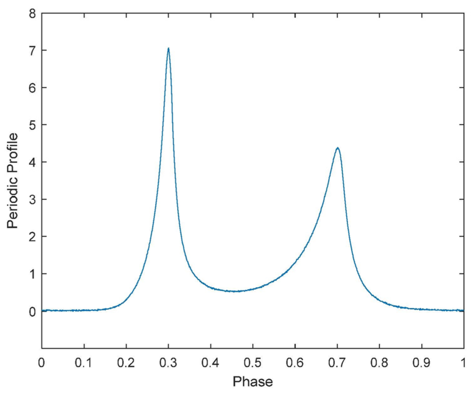
Here, the Crab pulsar with simulation parameters shown in Table 1 was taken as the observed pulsar. Figure 2 shows the template of Crab pulsar. The initial orbit elements of spacecraft A and spacecraft B are shown in Table 2. Both spacecraft were assumed to observe Crab pulsar with observation $t_{obs}=100 \mathrm{s}$. In this section, we assumed that the true position and velocity of spacecraft A was known, and the observation data of Crab pulsar were used to estimate state of spacecraft B with Algorithm 1. The initial state errors of spacecraft B were set as [5 km, 5 km, 5 km] and [5 m/s, 5 m/s, 5 m/s].

Table 1. Simulation parameters of Crab pulsar [29].

Parameters	Value
Period [ms]	33.4
$\alpha$ [ph/s]	660
$\beta$ [ph/s]	13,860.2

Figure 2. Template of the Crab pulsar.

Table 2. Orbital elements of spacecraft A and B.

Orbital Elements	Spacecraft A	Spacecraft B
Inclination/°	51.6995	63.2
Semi-major axis/km	6781.5888	6922.0854
Eccentricity	8.63 × 10−4	4.76 × 10−4
Right ascension of the ascending node/°	137.2927	252.4538
Argument of perigee/°	124.2185	121.7897
True anomaly/°	183.5224	279.4325

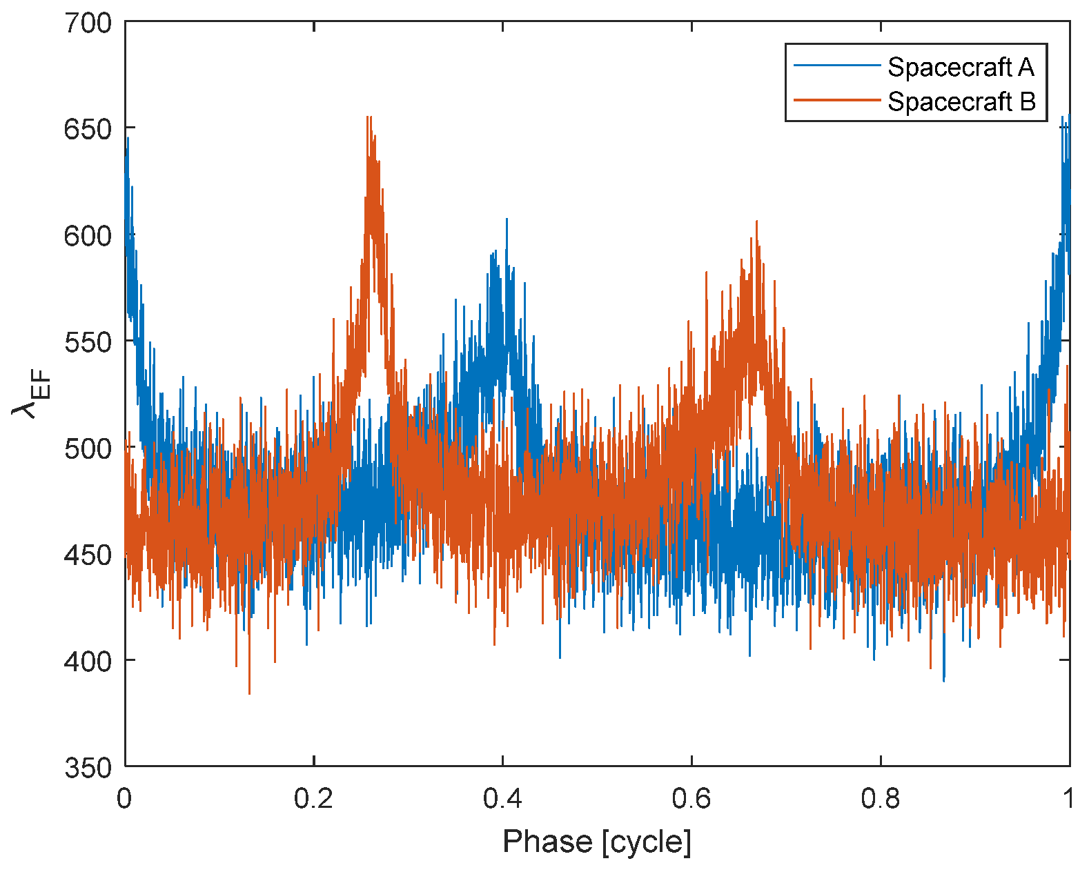
The initial state of spacecraft A and B was used to recover empirical profiles with $\left\{\varphi \right({\tau }_{j,SSB}^{HXMT}\left)\right\}$ and $\left\{\varphi \right({\tau }_{j,SSB}^{NICER}\left)\right\}$ via (13). The recovered empirical profiles are shown in Figure 3. Due to the distance between spacecraft A and B, pulse phase of Spacecraft A and B in the same exposure were different. Using (33) to estimate $\mathsf{\Delta }{\hat{\varphi }}_i^{A,B}$, the value of estimated pulse phase delay was 0.2650, and $\mathsf{\Delta }{\varphi }_i^{A,B}$, calculated by (29), was 0.2652. It can be seen that $\mathsf{\Delta }{\hat{\varphi }}_i^{A,B}$ was close to $\mathsf{\Delta }{\varphi }_i^{A,B}$, computed via (29). Therefore, the pulse phase delay can reflect the distance between spacecraft A and B.

Figure 3. Empirical profiles of spacecraft A and B.

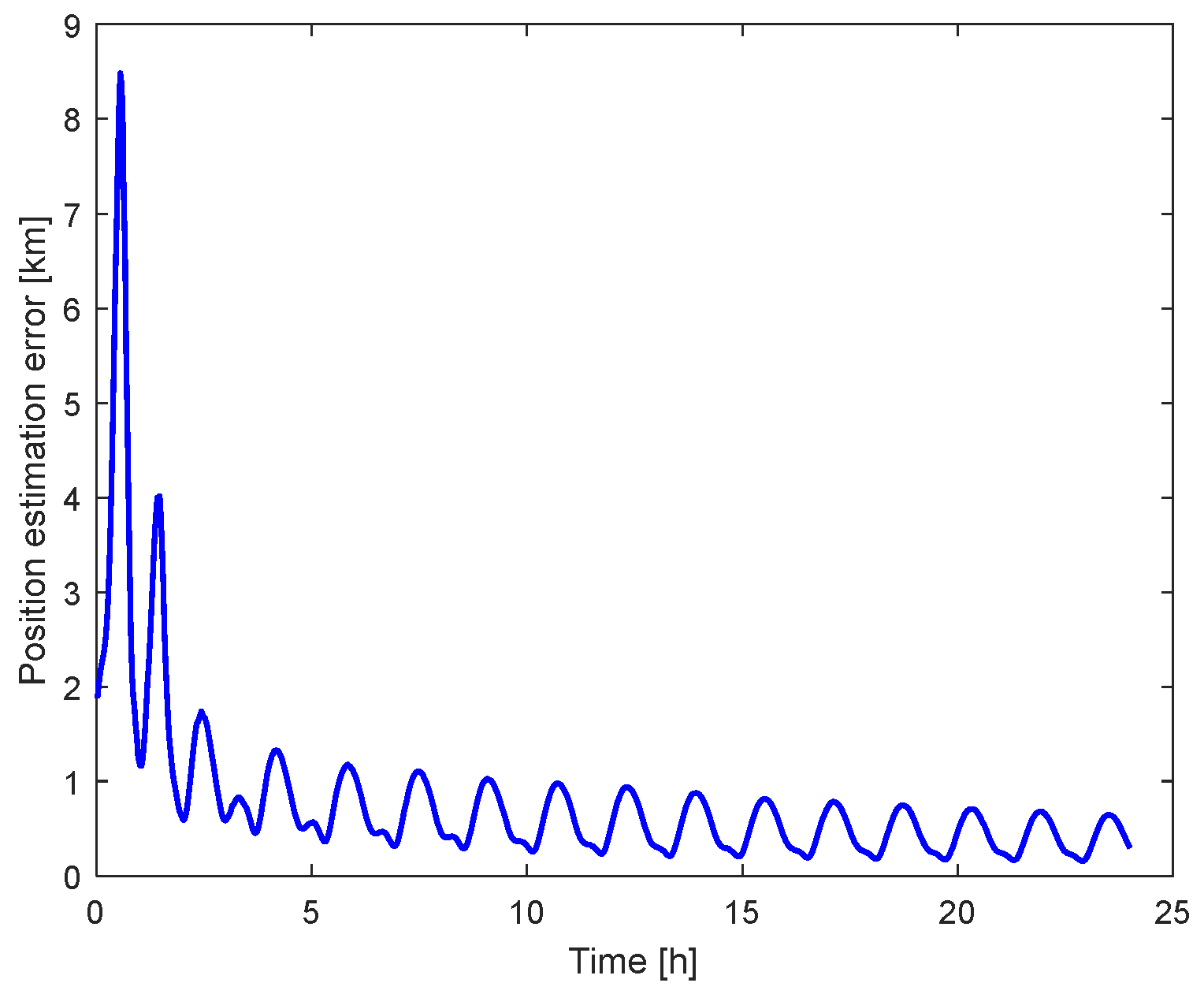
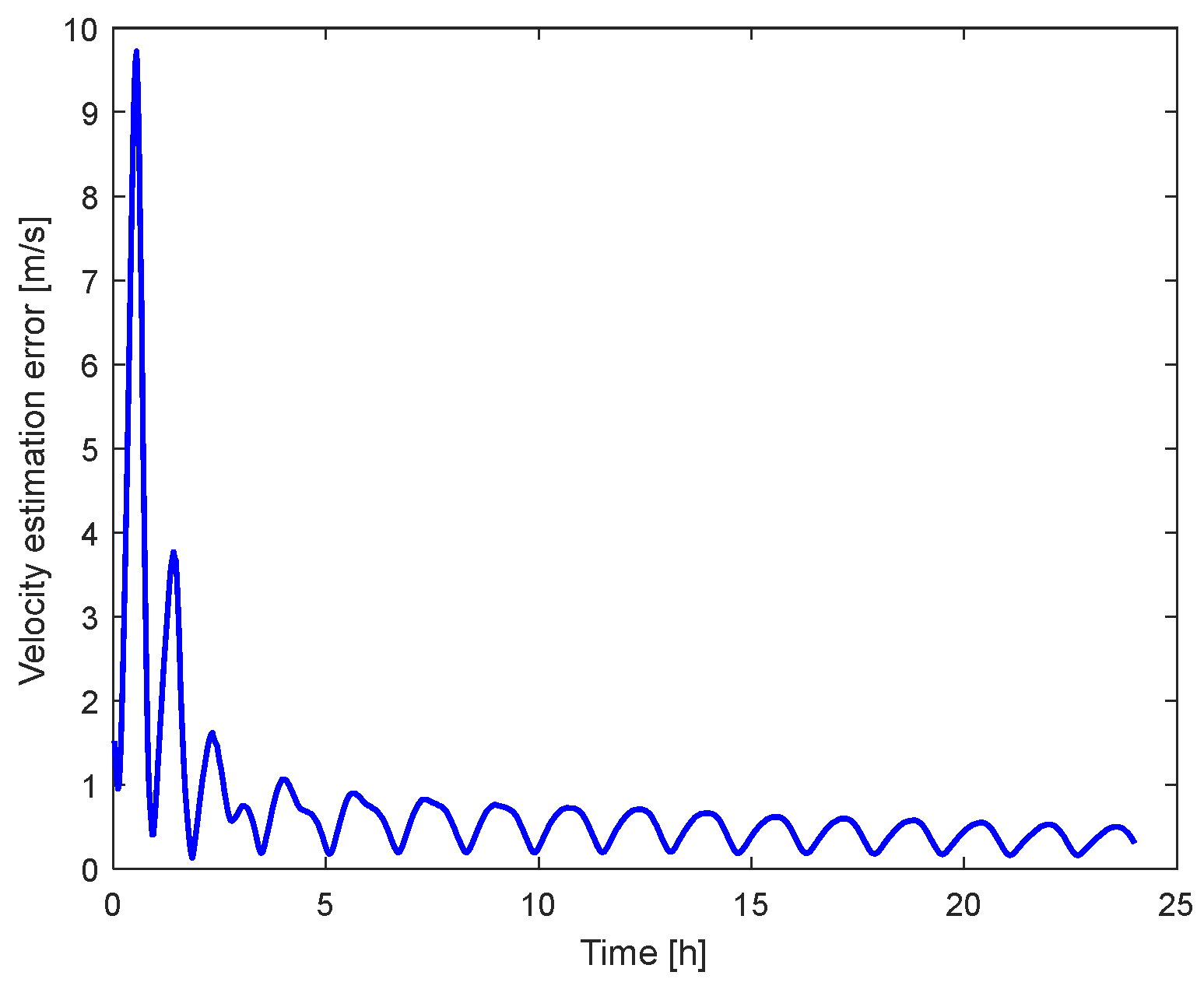
Figure 4 and Figure 5 show the navigation result of spacecraft B. As can be seen, the position and velocity gradually reduced to below 1 km and 1 m/s, respectively, thus verifying the feasibility of proposed navigation method using pulse phase delay.

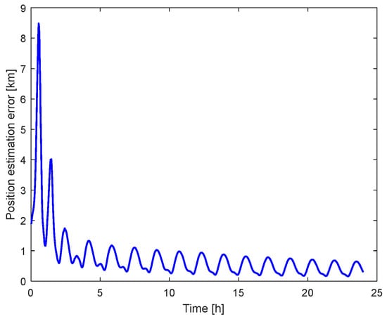
Figure 4. Position estimation error of spacecraft B.

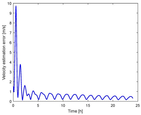
Figure 5. Velocity estimation error of spacecraft B.

4.2. Experiments with Real Data

We use real data of Crab pulsar from LE (Low Energy X-ray Telescope) on Insight-HXMT and NICER on 13 March 2018 and 14 March 2018 (Obs_ID: P0111605054 (Insight-HXMT), 1013010125 (NICER), and 1013010126 (NICER)). The start and finish time of real data are shown in Table 3.

Table 3. Start and finish time of real data.

Obs_ID	Start Time [UTC]	Finish Time [UTC]
P0111605054	13 March 2018 03:38:24	14 March 2018 18:02:10
1013010125	13 March 2018 02:58:15	13 March 2018 23:02:12
1013010126	13 March 2018 00:32:49	14 March 2018 14:58:16

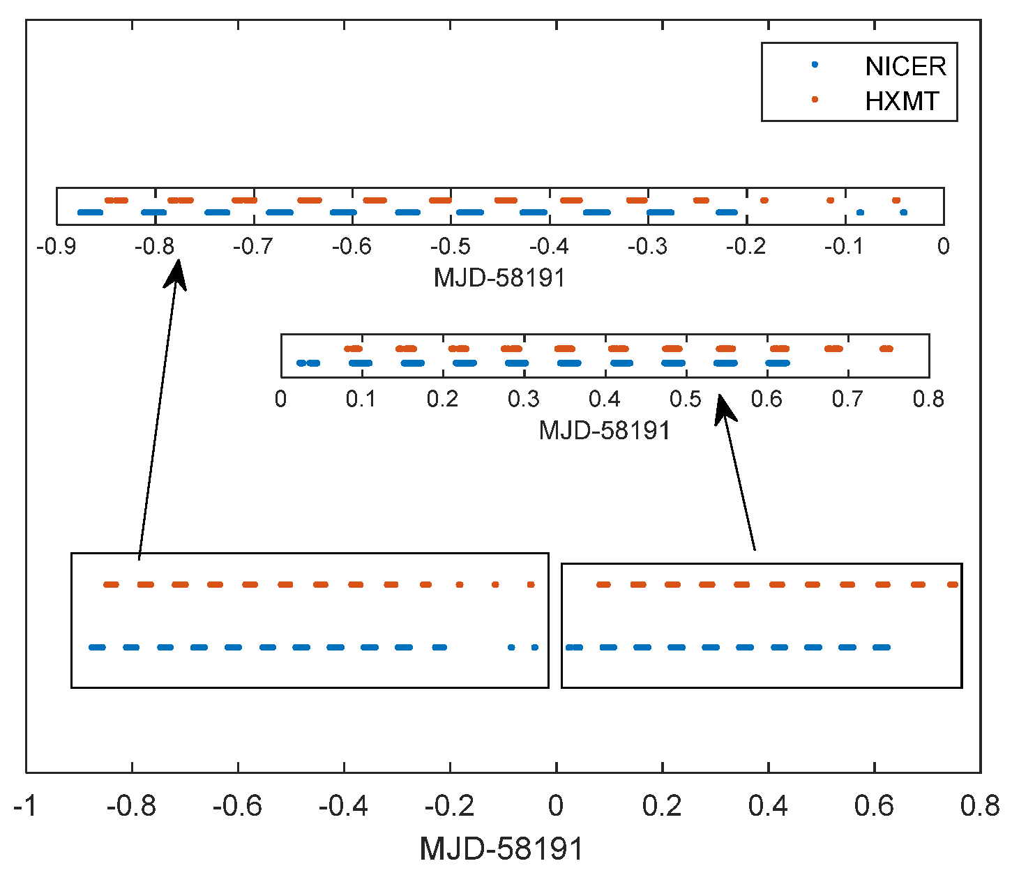
To verify the proposed pulsar-based navigation method using pulse phase delay, we chose the real data when Insight-HXMT and NICER simultaneously observe the Crab pulsar. The exposures on Crab pulsar from NICER and Insight-HXMT are shown in Figure 6. As shown in the figure, 13 March 2018 (MJD:58190) Insight-HXMT and NICER did not observe Crab pulsar simultaneously. On 14 March 2018 (MJD:58191), there are nine exposures that meet the criteria. We select these nine exposures and align the start time of each exposure. The start times of the selected exposures are shown in Table 4.

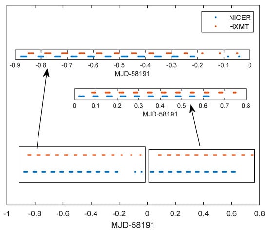
Figure 6. Exposure on Crab pulsar from Insight-HXMT and NICER.

Table 4. The start times of the selected nine exposures.

Number	Start Time [UTC]
1	14 March 2018 02:06:27
2	14 March 2018 03:40:51
3	14 March 2018 05:14:53
4	14 March 2018 06:43:16
5	14 March 2018 08:16:06
6	14 March 2018 09:50:46
7	14 March 2018 11:22:42
8	14 March 2018 12:58:12
9	14 March 2018 14:34:19

Given that there are only nine exposures in which Insight-HXMT and NICER simultaneously observe Crab pulsar, we verified the proposed pulsar-based navigation method by comparing pulse phase delay calculated by (28) and that estimated by (33). With the pulse phases of events received by Insight-HXMT and NICER, $\left\{\varphi \right({\tau }_{j,SSB}^{HXMT}\left)\right\}$ and $\left\{\varphi \right({\tau }_{j,SSB}^{NICER}\left)\right\}$ were calculated by (20) and (21) using the real position of NICER and Insight-HXMT. The empirical profiles of NICER and Insight-HXMT in each exposure were then recovered using $\left\{\varphi \right({\tau }_{j,SSB}^{HXMT}\left)\right\}$ and $\left\{\varphi \right({\tau }_{j,SSB}^{NICER}\left)\right\}$ via (13). The empirical profiles in each exposure are shown in Figure 7. Given the distance between NICER and Insight-HXMT in the direction of pulsar, the pulse phases of NICER and Insight-HXMT in the same exposure were different. In accordance with (24), the pulse phase delay $\mathsf{\Delta }{\hat{\varphi }}_i^{HXMT,NICER}$ reflects the distant between NICER and Insight-HXMT in the direction of the pulsar.

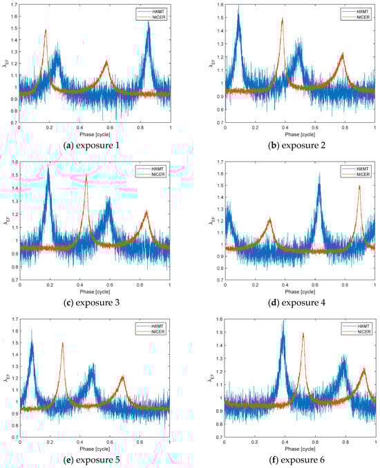
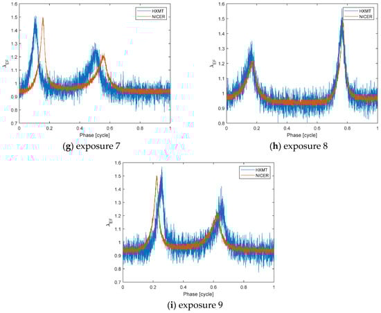
Figure 7. Empirical profiles of each exposure.

Next, we used the estimation error of $\mathsf{\Delta }{\hat{\varphi }}_i^{HXMT,NICER}$ to reflect the measurement error of the distance between Insight-HXMT and NICER. The pulse phase delays $\mathsf{\Delta }{\hat{\varphi }}_i^{HXMT,NICER},i=1,\dots ,9$ were estimated by (33) using the empirical profiles of NICER and Insight-HXMT shown in Figure 6. The real pulse phase delays were calculated by (28) using the real positions of NICER and Insight-HXMT. Furthermore, the estimation error of pulse phase delay was defined as the difference between estimated pulse phase delay and real pulse phase delay. Table 5 shows the estimation errors of the pulse phase delay of nine exposures. The results revealed that the estimated pulse phase delay can accurately reflect the distance between Insight-HXMT and NICER, thus verifying the feasibility of the proposed pulsar-based navigation using the pulse phase delay.

Table 5. Estimation errors of the pulse phase delay.

Exposure Number	Estimation Error [Cycle]
1	2.63 × 10−3
2	−2.82 × 10−3
3	2.80 × 10−3
4	3.89 × 10−4
5	−9.16 × 10−4
6	3.39 × 10−5
7	−2.51 × 10−3
8	−2.44 × 10−4
9	−1.42 × 10−4

Finally, we compared the performance of the separate estimation method for pulse phase delay used in (19) and the proposed direct estimation method. In the proposed direct estimation method, pulse phase delays $\mathsf{\Delta }{\hat{\varphi }}_i^{HXMT,NICER}, i=1,\dots ,9$ were directly estimated by (33) using the empirical profiles of Insight-HXMT and NICER in each exposure. In the respective estimation method, $\mathsf{\Delta }{\hat{\varphi }}_i^{HXMT}$ and $\mathsf{\Delta }{\hat{\varphi }}_i^{NICER}$ were estimated, respectively, by (19) using empirical profiles and templates, after which $\mathsf{\Delta }{\hat{\varphi }}_i^{HXMT,NICER}, i=1,\dots ,9$ were then calculated by (24). The evaluation criterion of the estimation performance is defined as RMS (root mean square) error of the pulse phase delay. We defined CPU time cost as evaluation criterion of computational cost. The computation environment contained Intel Core i5-1240P@1.7 GHZ (Intel, Santa Clara, CA, USA) and python 3.8. Table 6 shows the RMS error and mean CPU time cost of the proposed direct estimation method and the separate estimation method for pulse phase delay. The results showed that the estimation performance of the proposed direct estimation method was close to that of respective estimation method. Furthermore, the CPU time cost of the proposed direct estimation method was about 36.99% lower than that of respective estimation method.

Table 6. RMS error and mean CPU time cost for different pulse phase delay estimation methods.

Method	RMS Error [cycle]	Mean CPU Time Cost [s]
Proposed direct estimation method	1.83 × 10−3	0.0092
Respective estimation method	1.71 × 10−3	0.0146

5. Conclusions

This study derived a pulsar-based navigation method using pulse phase delay between spacecraft. A direct estimation method for pulse phase delay is proposed to eliminate reliance on templates of pulsars for pulse phase delay estimation. The proposed method is verified with the simulation data of the Crab pulsar and the real data of the Crab pulsar form Insight-HXMT and NICER. Real data experiment results show that the pulse phase delay estimated by the real data of the Crab pulsar can accurately reflect the distance between Insight-HXMT and NICER. Moreover, compared with the estimation method that estimates the pulse phase of two spacecraft, the proposed direct estimation method can estimate pulse phase delay between two spacecraft by running the pulse phase estimation algorithm just once. The experimental results show that the estimation performance of the proposed direct estimation method is close to that of the respective estimation method and that the CPU time cost of the proposed method is about 36.99% lower. Notably, the transform model shown as (2) only considers the Romer delay and Shapiro delay. An accurate transform model that considers the Einstein delay and high-order terms of relativistic effects should be considered in further studies to provide an accurate navigation service for spacecraft near gravitational sources.

References

- Fraser, C.T.; Ulrich, S. Adaptive extended Kalman filtering strategies for spacecraft formation relative navigation. Acta Astronaut. 2021, 178, 700–721. [Google Scholar] [CrossRef]
- Vasile, M.; Torre, F.; Serra, R.; Grey, S. Autonomous orbit determination for formations of Cubesats beyond LEO. Acta Astronaut. 2018, 153, 327–336. [Google Scholar] [CrossRef]
- Scharnagl, J.; Haber, R.; Dombrovski, V.; Schilling, K. NetSat—Challenges and lessons learned of a formation of 4 nano-satellites. Acta Astronaut. 2022, 201, 580–591. [Google Scholar] [CrossRef]
- Yang, C.; Zhang, H.; Gao, Y. Analysis of a neural-network-based adaptive controller for deep-space formation flying. Adv. Space Res. 2021, 68, 54–70. [Google Scholar] [CrossRef]
- Wang, X.; Gong, D.; Jiang, Y.; Mo, Q.; Kang, Z.; Shen, Q.; Wu, S.; Wang, D. A Submillimeter-Level Relative Navigation Technology for Spacecraft Formation Flying in Highly Elliptical Orbit. Sensors 2020, 20, 6524. [Google Scholar] [CrossRef]
- Zink, M.; Moreira, A.; Hajnsek, I.; Rizzoli, P.; Bachmann, M.; Kahle, R.; Fritz, T.; Huber, M.; Krieger, G.; Lachaise, M.; et al. TanDEM-X: 10 Years of Formation Flying Bistatic SAR Interferometry. IEEE J. Sel. Top. Appl. Earth Obs. Remote Sens. 2021, 14, 3546–3565. [Google Scholar] [CrossRef]
- Wang, S.; He, C.; Gong, B.; Ding, X.; Yuan, Y. Cooperative Angles-Only Relative Navigation Algorithm for Multi-Spacecraft Formation in Close-Range. Comput. Model. Eng. Sci. 2023, 134, 121–134. [Google Scholar] [CrossRef]
- Liu, J.; Fang, J.; Yang, Z.; Kang, Z.-W.; Wu, J. X-ray pulsar/Doppler difference integrated navigation for deep space exploration with unstable solar spectrum. Aerosp. Sci. Technol. 2015, 41, 144–150. [Google Scholar] [CrossRef]
- Wang, Y.; Zheng, W.; Sun, S.; Li, L. X-ray pulsar-based navigation using time-differenced measurement. Aerosp. Sci. Technol. 2014, 36, 27–35. [Google Scholar] [CrossRef]
- Wang, Y.; Zheng, W.; Zhang, S.; Ge, M.; Li, L.; Jiang, K.; Chen, X.; Zhang, X.; Zheng, S.; Lu, F. Review of X-ray pulsar spacecraft autonomous navigation. Chin. J. Aeronaut. 2023, 36, 44–63. [Google Scholar] [CrossRef]
- Chen, P.-T.; Bayard, D.S.; Sharrow, R.F.; Majid, W.A.; Dunst, B.A.; Speyer, J.L. A Gaussian Sum Filter for Pulsar Navigation: Processing Single Photon Arrival Time Measurements. IEEE Trans. Contr. Syst. Technol. 2023, 31, 2499–2514. [Google Scholar] [CrossRef]
- Sheikh, S.I.; Pines, D.J.; Ray, P.S.; Wood, K.S.; Lovellette, M.N.; Wolff, M.T. Spacecraft Navigation Using X-Ray Pulsars. J. Guid. Control Dyn. 2006, 29, 49–63. [Google Scholar] [CrossRef]
- Winternitz, L.B.; Hassouneh, M.A.; Mitchell, J.W.; Price, S.R.; Yu, W.H.; Semper, S.R.; Ray, P.S.; Wood, K.S.; Arzoumanian, Z.; Gendreau, K.C. SEXTANT X-ray Pulsar Navigation Demonstration: Additional On-Orbit Results. In Proceedings of the 2018 SpaceOps Conference, Marseille, France, 28 May–1 June 2018. [Google Scholar]
- Zheng, S.J.; Zhang, S.N.; Lu, F.J.; Zheng, W.; Chen, X.; Zheng, S.; Lu, F. In-orbit demonstration of X-ray pulsar navigation with the Insight-HXMT satellite. Astrophys. J. Suppl. Ser. 2019, 244, 1. [Google Scholar] [CrossRef]
- Zheng, S.J.; Zhang, S.N.; Lu, F.J.; Wang, W.B.; Gao, Y.; Li, T.P.; Song, L.M.; Ge, M.Y.; Han, D.W.; Chen, Y.; et al. Fast On-Orbit Pulse Phase Estimation of X-Ray Crab Pulsar for XNAV Flight Experiments. IEEE Trans. Aerosp. Electron. Syst. 2022, 59, 3395–3404. [Google Scholar]
- Wang, Y.; Zheng, W.; Ge, M.; Zheng, S.; Zhang, S.; Lu, F. Use of Statistical Linearization for Nonlinear Least-Squares Problems in Pulsar Navigation. J. Guid. Control Dyn. 2023, 46, 1850–1856. [Google Scholar] [CrossRef]
- Xiong, K.; Wei, C.L.; Liu, L.D. The use of X-ray pulsars for aiding navigation of satellites in constellations. Acta Astronaut. 2009, 64, 427–436. [Google Scholar]
- Zhang, H.; Jiao, R.; Xu, L.P.; Xu, C.; Mi, P. Formation of a Satellite Navigation System Using X-Ray Pulsars. Publ. Astron. Soc. Pac. 2019, 131, 045002. [Google Scholar]
- Emadzadeh, A.A.; Speyer, J.L. X-Ray Pulsar-Based Relative Navigation using Epoch Folding. IEEE Trans. Aerosp. Electron. Syst. 2011, 47, 2317–2328. [Google Scholar] [CrossRef]
- Zhou, Q.Y.; Ji, J.F.; Ren, H.F. Timing equation in X-ray pulsar autonomous navigation. Acta Phys. Sin. 2013, 62, 139701. [Google Scholar] [CrossRef]
- Lyne, A.G.; Pritchard, R.S.; Graham Smith, F. 23 Years of Crab Pulsar Rotational History. Mon. Not. R. Astron. Soc. 1993, 265, 1003–1012. [Google Scholar] [CrossRef]
- Edwards, R.T.; Hobbs, G.B.; Manchester, R.N. TEMPO2, a new pulsar timing package—II. The timing model and precision estimates. Mon. Not. Roy. Astron. Soc. 2006, 372, 1549–1574. [Google Scholar] [CrossRef]
- Emadzadeh, A.A.; Speyer, J.L. On Modeling and Pulse Phase Estimation of X-ray Pulsars. IEEE Trans. Signal Process 2010, 58, 4484–4495. [Google Scholar] [CrossRef]
- Wang, Y.; Zheng, W. Pulse Phase Estimation of X-ray Pulsar with the Aid of Vehicle Orbital Dynamics. J. Navig. 2016, 69, 414–432. [Google Scholar] [CrossRef]
- Wang, Y.; Zhang, W. Pulsar phase and Doppler frequency estimation for XNAV using on-orbit epoch folding. IEEE Trans. Aerosp. Electron. Syst. 2016, 52, 2210–2219. [Google Scholar] [CrossRef]
- Robert, G.M. Fundamentals of Astrodynamics and Applications. J. Guid. Control Dyn. 1998, 21, 803–812. [Google Scholar]
- Wang, Y.S.; Wang, Y.D.; Jiang, K.; Zheng, W.; Song, M. Adaptive Grid Search Based Pulse Phase and Doppler Frequency Estimation for XNAV. IEEE Trans. Aerosp. Electron. Syst. 2024, 60, 3707–3717. [Google Scholar] [CrossRef]
- Sun, H.; Su, J.; Deng, Z.; Shen, L.; Bao, W.; Li, X.P.; Li, L.; Su, Z.; Wang, W. Grouping bi-chi-squared method for pulsar navigation experiment using observations of Rossi X-ray timing explorer. Chin. J. Aeronaut. 2022, 36, 386–395. [Google Scholar] [CrossRef]
- Winternitz, L.M.B.; Hassouneh, M.A.; Mitchell, J.W.; Valdez, J.E.; Price, S.R.; Semper, S.R.; Yu, W.H.; Ray, P.S.; Wood, K.S.; Arzoumanian, Z.; et al. X-ray pulsar navigation algorithms and testbed for SEXTANT. In Proceedings of the 2015 IEEE Aerospace Conference, Big Sky, MT, USA, 7–14 March 2015. [Google Scholar]
Disclaimer/Publisher’s Note: The statements, opinions and data contained in all publications are solely those of the individual author(s) and contributor(s) and not of MDPI and/or the editor(s). MDPI and/or the editor(s) disclaim responsibility for any injury to people or property resulting from any ideas, methods, instructions or products referred to in the content. |
© 2024 by the authors. Licensee MDPI, Basel, Switzerland. This article is an open access article distributed under the terms and conditions of the Creative Commons Attribution (CC BY) license (https://creativecommons.org/licenses/by/4.0/).