BESO and SESO: Comparative Analysis of Spatial Structures Considering Self-Weight and Structural Reliability

Abstract

A comparative analysis between Bidirectional Evolutionary Structural Optimization (BESO) and Smoothing-ESO (SESO), simultaneously considering Reliability-Based Topology Optimization (RBTO) and the structure’s self-weight in the case of three-dimensional elasticity, is presented in this study. Due to the important role of the existence of uncertainties in making the structural design more realistic, geometry, volumetric fraction, modulus of elasticity, compliance, and loading are considered random variables with normal probability distribution. When adopting the First Order Reliability Method (FORM), the failure probability is calculated based on the reliability index. Furthermore, considering the influence of self-weight in problems involving large structures in civil engineering, especially in the case of bridges, this makes the optimal configuration more reliable for design. A series of examples are covered to validate the methods presented, showing their efficiency and robustness.

1. Introduction

Topological Optimization (TO) is a technique used to find the ideal distribution of the material in a structure, maximizing its performance under certain constraints. In recent decades, this approach has been used by several researchers in the field of structural engineering to reduce weight, improve efficiency, and increase the strength of materials. As algorithms evolve, this technique has played an important role in the production of complex and innovative structures, contributing to the advancement of civil, aerospace, mechanical, and naval engineering. However, many TO designs do not consider the structure’s self-weight, which can be a problem when considering large structures in civil engineering, especially in the case of bridges, viaducts, large buildings, and towers.

Several methods have been developed for OT, including the Moving Asymptote Method by [1] the density-based Solid Isotropic Material Penalty (SIMP) by [2,3], the Bubble Method by [4], and the Level-Set Method, by [5,6,7]. In this article, we highlight evolutionary methods such as Evolutionary Structural Optimization (ESO) by [8,9,10], and Bidirectional Evolutionary Structural Optimization (BESO) by [11,12,13], and ESO Smoothing, called SESO, by [14,15].

In this article, a comparative analysis of three-dimensional elastic structures is proposed between the methods: (a) BESO, which was developed from ESO, and has a bidirectional optimization procedure, allowing the addition and removal of inefficient elements of the structure. This method is efficient and robust and has been successfully applied to a wide variety of OT problems for two-dimensional structures, including compliance minimization by [16,17], frequency maximization, and displacement constraint by [18]. BESO for compliance minimization was applied to three-dimensional structures by [19], who presented a code in Python; [16] applied it to strut-and-tie models and [20] in continuous structures with self-supporting geometric constraints. Ref. [21] extened the BESO method to the RBTO of three-dimensional structures, considering an elastic-plastic topology optimization. Ref. [22] used BESO for RBTO for 3D structures in conjunction with the standard response surface method and (b) SESO, which is also a bidirectional TO procedure and is efficient and robust in several problems with restriction of displacement, voltage, compliance, and frequency. Recently, it was extended to spatial structures in the work of [23,24], which uses as a restriction the minimization of compliance coupled with the reliability analysis procedure via the FORM method, considering geometry, elastic modulus, compliance, force, and von Mises stress as random variables with normal probability distribution.

For comparative analysis, RBTO-BESO (Reliability-Based Topology Optimization BESO) and RBTO-SESO (Reliability-Based Topology Optimization SESO) were implemented, inserting the structure’s self-weight, making the optimal configurations more realistic in structural design. Furthermore, the proposed algorithm can determine the tensile (blue) and compression (red) regions in the optimized structure using a modal filter and the partial derivative of the von Mises stress field. After identifying the sign of the derivatives, a radius is defined for the filter, which aims to search neighboring elements in relation to their state (traction or compression). This approach allows, in regions with many tensioned/compressed elements, that the presence of a single tensioned/compressed element is considered insignificant and, therefore, neglected by the algorithm, since it is in a region with tensioned/compressed neighbors. This technique provides smoothing of the regions, making them clearer and cleaner in terms of traction and compression, which significantly contributes to the robustness and effectiveness of the optimization process.

As BESO is a more stable method compared to ESO and its variants, a comparative analysis between BESO and SESO is necessary. SESO, a variant of ESO employing a bidirectional heuristic similar to BESO, warrants such scrutiny. This article expands on previous efforts to enhance the SESO-3D method, proposing a computational algorithm that integrates RBTO while considering the structure’s self-weight. Considering self-weight in TO impacts mass distribution, internal forces, and dynamic performance, thereby enhancing safety, reliability, and material efficiency in design.

Compared to other topology optimization methods like gradient-based approaches (such as the projected gradient method) or linear programming-based methods, BESO and SESO offer a bidirectional heuristic approach that allows for material addition and removal. This approach is particularly suitable for addressing complex problems with multiple optimization criteria and is easy to implement. However, these methods may require higher computational resources to achieve optimal results and are sensitive to parameters such as RR (rejection ratio), ER (evolutionary ratio), and filter size, which can affect optimization efficiency and accuracy.

The remainder of the article is organized as follows: In Section 2, the formulation for topological optimization considering the self-weight is described in general terms for the methods, including the formulation of the structure’s self-weight. Section 3 contains the RBTO formulation in general and with the consideration of self-weight and sensitivity analysis to determine the tensile and compression regions. Then, in Section 4, the examples presented are: cantilever to validate the formulation of the tensile and compressed regions, a natural optimization under the action of only the structure’s self-weight with the aim of validating the procedure and the examples of bridges in Section 5. Finally, conclusions are drawn.

2. SESO—Subject to Self-Weight Loads

The SESO method aims to optimize structural efficiency by removing or adding elements to the structure. In the search for the topology of maximum stiffness, it is common to use the minimization of the compliance or the maximum von Mises stress as an objective function, while the constraint is imposed on the structural weight, limiting the maximum volume of material allowed. Compliance represents the work done by the loads applied in the structure’s equilibrium state. An alternative approach to maximum stiffness design is to use elastic strain energy as a measure of structural stiffness. Therefore, the compliance minimization problem can be reformulated as a problem of minimizing the total elastic strain energy. Thus, the formulation of the TO problem can be defined as

$$\begin{array}{cc}\mathrm{M}\mathrm{i}\mathrm{n}\mathrm{i}\mathrm{m}\mathrm{i}\mathrm{z}\mathrm{e}:& \mathrm{C}\left(\mathit{x}\right)=U^T\left(\mathit{x}\right)K\left(\mathit{x}\right)U\left(\mathit{x}\right)\\ \mathrm{S}\mathrm{u}\mathrm{b}\mathrm{j}\mathrm{e}\mathrm{c}\mathrm{t} \mathrm{t}\mathrm{o}:& K\left(\mathit{x}\right)U\left(\mathit{x}\right)=F\left(\mathit{x}\right)\\ & F\left(\mathit{x}\right)=f^{ext}\left(\mathit{x}\right)+f^{grav}\left(\mathit{x}\right)\\ & V\left(\mathit{x}\right)={\sum }_{i=1}^{NE}{x}_i{V}_i-V^{\ast }\le 0\\ & \mathit{x}=\left\{x_1{ x}_{2 }{x}_{3 }\dots x_n\right\}, x_i=1 or x_i={10}^{-9}\end{array}$$

(1)

where C(x) is the objective function, $U\left(\mathit{x}\right)$ is the nodal displacement vector, $K\left(\mathit{x}\right)$ is the global stiffness matrix and $V_i$ is the volume of the element, and V* is the prescribed volume. $K\left(\mathit{x}\right)U\left(\mathit{x}\right)=F\left(\mathit{x}\right)$ is the equilibrium equation, $F\left(\mathit{x}\right)$ is the global force vector, $f^{ext}\left(\mathit{x}\right)$ is the external force vector, and $f^{grav}\left(\mathit{x}\right)$ is the force vector inertia forces of the structure, $x_i$ is the design variable of the i-th element, and $\mathit{x}$ is the vector of design variables. The design is binary and $x_i={10}^{-9}$ is imposed in order to avoid a singular FEM problem when solving the equilibrium.

To start the SESO process, it is necessary to define a problem that specifies a design domain and boundary conditions. Then, a finite element analysis is performed to determine the stiffness distribution. The heuristic of SESO is that the structure evolves into a stationary optimal solution, systematically removing inefficient elements. Through a sensitivity analysis, it is possible to calculate a sensitivity number ${\alpha }_j$ for each element, which indicates the magnitude of the change in global elastic strain energy resulting from the removal of that element. Elements with a low sensitivity number can be removed without significantly affecting the overall stiffness of the structure. The steps of the SESO method can be summarized according to the flowchart, as seen in Figure 1.

Formulation for Self-Weight Structure

Self-weight loads depend on gravitational acceleration and material properties, in particular, material density. As such, in OT problems formulated with SESO-3D approaches, the self-weight loads also depend on the set of design variables. Thus, it is possible to calculate and apply the self-weight at the nodes of the elements, and the main advantage is that the load is directly proportional to the amount of material used in the structure. For the hexahedral element proposed by [25], a gravitational load is obtained by assigning 1/8 of the element’s weight to each node according to Equation (2), whose formulation was proposed in [26].

$$f_i^{grav}={\rho }_i\ast V_i\ast g\ast \overline{f}={\displaystyle \frac{1}{8}}{dx}_i{dy}_i{dz}_i{\rho }_{i}g\overline{f}$$

(2)

where ${\rho }_i$ is the density of the i-th element, $g$ is the acceleration of gravity ($g=9.81 \mathrm{m}/{\mathrm{s}}^2)$, and $\overline{f}$ is given by

$$\overline{f}={\left[\begin{array}{cc}{\overline{f}}_1& {\overline{f}}_2\end{array} \begin{array}{ccc}{\overline{f}}_3& {\overline{f}}_4& {\overline{f}}_5\end{array} \begin{array}{ccc}{\overline{f}}_6& {\overline{f}}_7& {\overline{f}}_8\end{array}\right]}^T$$

(3)

with ${\overline{f}}_n$ is expressed by the nodal coordinates as:

$${\overline{f}}_n=\left[\begin{array}{ccc}0& -1& 0\end{array}\right] \mathrm{c}\mathrm{o}\mathrm{m} n=1, 2, 3, \dots , 8$$

(4)

Thus $f^{grav}$ defined in Equation (5) can be expressed as

$$f^{grav}=\sum _{i=1}^N{f}_i^{grav}$$

(5)

It is worth noting that the self-weight of the structure plays a significant role in structural behavior. For example, in structures where self-weight represents a significant fraction of the total loads, such as in tall buildings, bridges, and large infrastructure components, self-weight not only affects the distribution of stresses and deformations but also directly influences the stability and efficiency of the final design. The coupling of the Structural Reliability procedure ensures that the inherent uncertainties and variabilities in material behavior and loading conditions are considered, providing an additional layer of robustness to the optimization process. Therefore, coupling SESO-3D with RBTO and self-weight not only makes the optimization procedure more realistic but also improves the efficiency and applicability of the resulting structural designs.

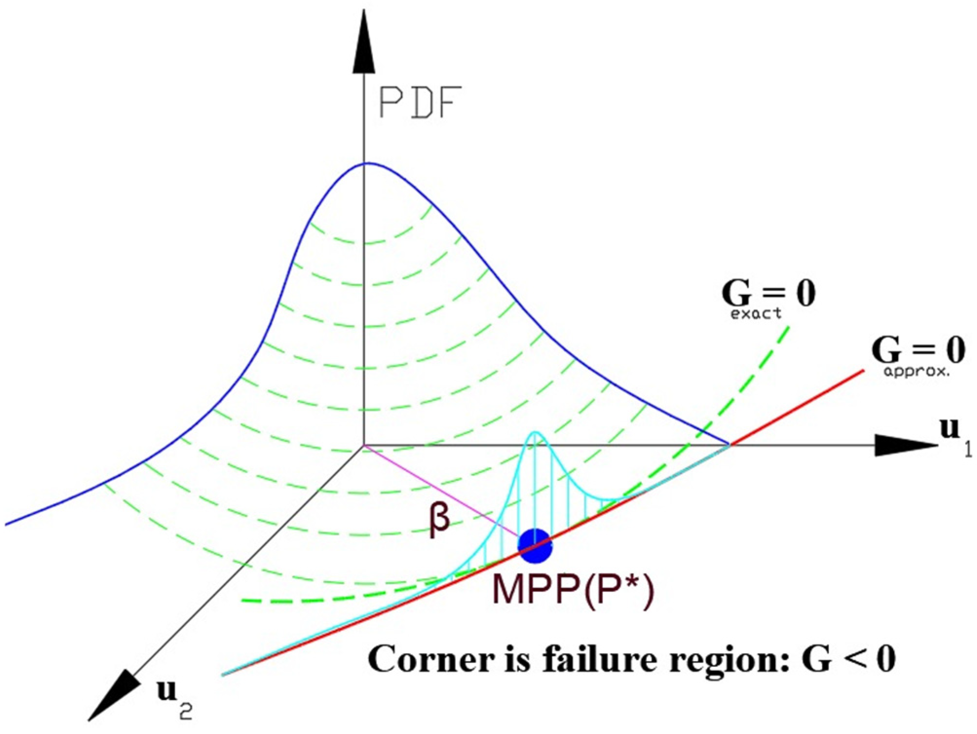
3. Reliability Analysis

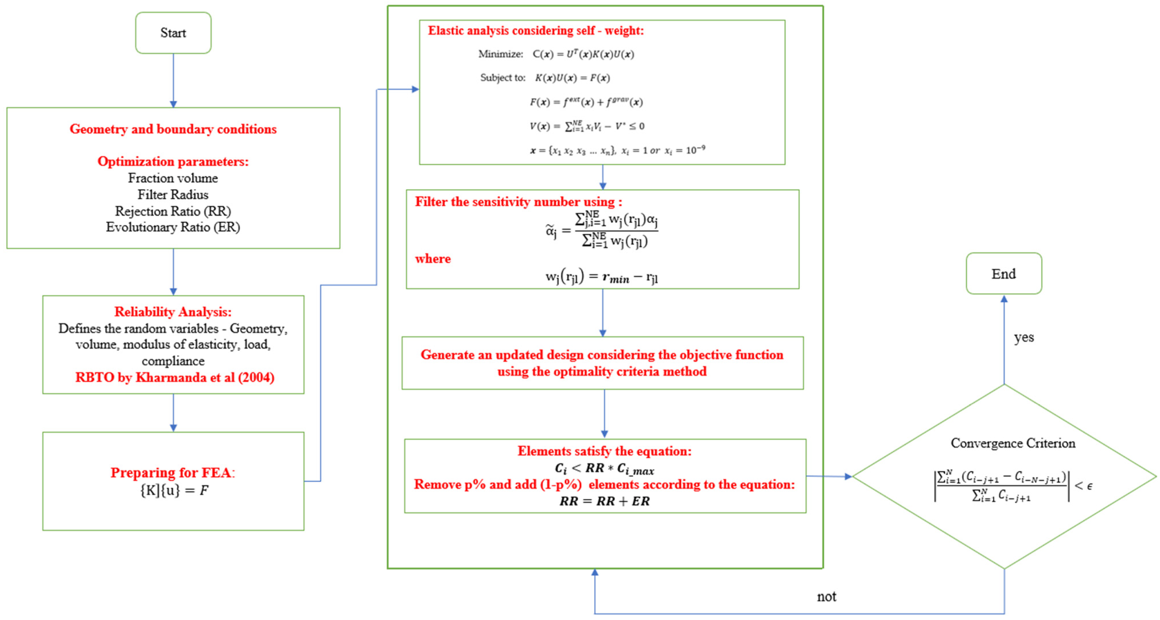
3.1. Formulation of the RBTO

Reliability analysis and design optimization are effective methods to ensure structural safety, as demonstrated by [27,28,29]. For the mathematical model of RBTO, it is sufficient to transform the stress constraint in Equation (6) as follows:

$$\begin{array}{cc}\mathrm{M}\mathrm{i}\mathrm{n}\mathrm{i}\mathrm{m}\mathrm{i}\mathrm{z}\mathrm{e}& V(x_i,{\mathit{X}}_j,\mathit{u})={\sum }_{i=1}^{NE}{x}_i{V}_i(x_i,{\mathit{X}}_j,\mathit{u})\\ \mathrm{s}\mathrm{u}\mathrm{b}\mathrm{j}\mathrm{e}\mathrm{c}\mathrm{t} \mathrm{t}\mathrm{o}& P_f=\mathrm{P}\left[G\left(x_i,{\mathbf{X}}_j\right)\le 0\right]=\int \dots {\int }_{G\left(x_i, X\right)\le 0}{f}_X\left(\mathbf{X}\right)dx\\ & \mathrm{K}(x_i,{\mathit{X}}_j,\mathit{u})\mathrm{U}(x_i,{\mathit{X}}_j,u)=\mathrm{F}({\mathit{X}}_j,\mathit{u})\\ & \beta \left(\mathit{u}\right)={\beta }_t\\ & x_i=1 or x_i={10}^{-9} \mathrm{w}\mathrm{i}\mathrm{t}\mathrm{h} i=1, \dots , NE and j=1, \dots , m \end{array}$$

(6)

with $x_i$ being the finite element, ${\mathit{X}}_j$ is the j-th random variable, V is the volume of the total structure, $P_f$ is the probability of failure, G is the limit state function, and NE is the number of variables and m the number of uncertain variables. To control the topologies obtained by the RBTO model, the reliability index $\beta \left(\mathit{u}\right)$, see [30], is introduced with a normalized vector $\mathit{u}$.

$$G\left(x_i,{\mathrm{X}}_j\right)=R-S={\sigma }^{\ast }-{\sigma }_e^{vm}(x_i,{\mathrm{X}}_j)$$

(7)

where $R$ denotes the structural strength and S denotes the load variable. In this paper, we consider the possibility that random variables may cause the von Mises stress to exceed the yield strength limit of the material, thus causing the failure of the structure. Here, R indicates the allowable stress for the material $\left({\sigma }^{\ast }\right)$ and S indicates the von Mises stress of the element ${\sigma }_e^{vm}(x_i,{\mathit{X}}_j)$. Thus, if $G>0$, the structure is reliable, if $G<0$, the structure fails, and if $G=0$, the structure is in the limit state.

3.2. Formulation of the RBTO Problem Considering the Self-Weight

The objective of analyzing strut-and-tie models using the TO strategy is to find a reinforcement arrangement within the design domain that minimizes the maximum von Mises stress of the structure for given loading and boundary conditions. Mathematically, the problem can be stated as

$$\begin{array}{cc}\mathrm{M}\mathrm{i}\mathrm{n}\mathrm{i}\mathrm{m}\mathrm{i}\mathrm{z}\mathrm{e}& V=\sum _{e=1}^{ne}{x}_e{V}_e \\ \mathrm{s}\mathrm{u}\mathrm{b}\mathrm{j}\mathrm{e}\mathrm{c}\mathrm{t} \mathrm{t}\mathrm{o}& K\left(\mathit{x}\right)U\left(\mathit{x}\right)=F\left(\mathit{x}\right)\\ & F\left(\mathit{x}\right)=f^{ext}\left(\mathit{x}\right)+f^{grav}\left(\mathit{x}\right)\\ & {\sigma }_e^{vm}-{\sigma }^{\ast }\le 0\\ & V\left(\mathit{x}\right)={\sum }_{i=1}^{NE}{x}_i{V}_i-\mathrm{V}\le 0\\ & \beta \left(\mathit{u}\right)={\beta }_t\\ & \mathit{x}=\left\{x_1{ x}_{2 }{x}_{3 }\dots x_n\right\}, x_i=1 or x_i={10}^{-9}\end{array}$$

(8)

where ${\beta }_t$ is the target reliability index and ${\sigma }_e^{vm}$ the von Mises stress on each element is calculated using Equation (9).

$${\sigma }_e^{vm}={\left[{\sigma }_x^2+{\sigma }_y^2+{\sigma }_z^2-{\sigma }_x{\sigma }_y-{\sigma }_x{\sigma }_z-{\sigma }_y{\sigma }_z+3{\tau }_{xy}^2+{3\tau }_{xz}^2{+3\tau }_{yz}^2\right]}^{1/2}$$

(9)

where $V$ is the volume of the whole structure, $V_e$ is the volume of the e-th element, $K$ is the stiffness matrix of the structure, $U$ is the displacements vector, $F$ is the force vector, ne is the total number of finite elements of the structure, ${\sigma }_e^{vm}$ is the von Mises stress of element e, ${\sigma }^{\ast }$ is an admissible stress, $x_e=0$ denotes empty material, and $x_e=1$ denotes solid material. This formulation shows that the optimization procedure aims to minimize the number of elements and therefore minimize the volume of the structure. This structure is subject to the equilibrium equations as well as a stress constraint for each element that must be less than or equal to the permissible stress.

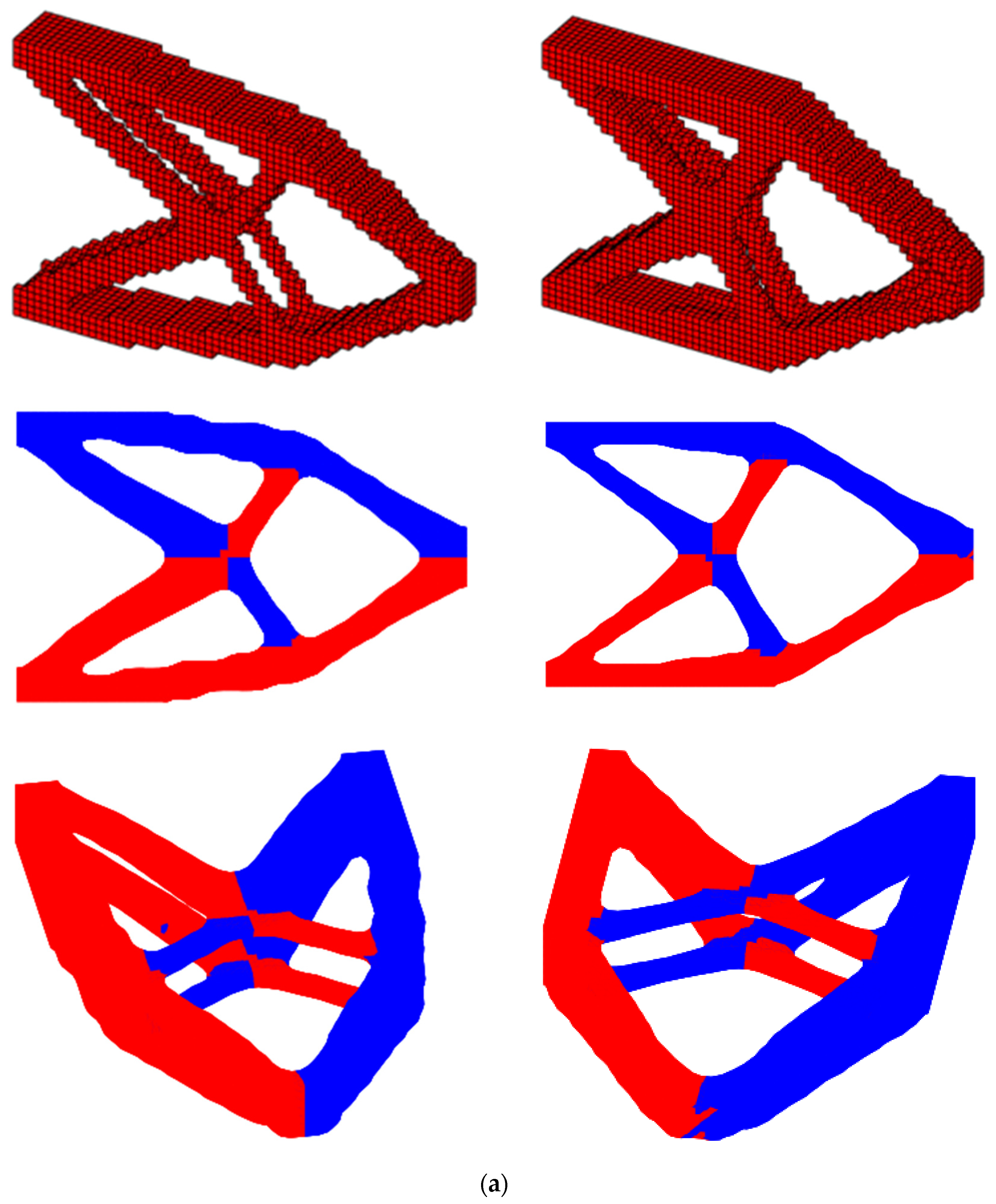
3.3. Sensitivity Analysis and Principal Stress for Determining Tensile and Compression Regions

3.3.1. Tensile and Compressive State

During the topological optimization procedure, the sum of the main stresses of each element will be used as a criterion to establish the predominant state of tension and compression. Thus, we have the following:

(1)

If ${\sigma }_1+{\sigma }_2+{\sigma }_3>0$ this indicates that the mean stress is positive, suggesting a predominantly tensile state.

(2)

If ${\sigma }_1+{\sigma }_2+{\sigma }_3<0$ this indicates that the mean stress is negative, suggesting a predominantly compressive state.

The above is as proposed by [31], where ${\sigma }_1$, ${\sigma }_2$, and ${\sigma }_3$ are the first principal stress, the second principal stress and the third principal stress of the element, respectively.

3.3.2. Derivative Sign Analysis: Sensitivity Analysis

Taking the local calculation of the derivative of the von Mises stress of the element with respect to the components of the stress vector described respectively as

$$\begin{array}{c}{\displaystyle \frac{\partial \left({\sigma }_e^{vm}\right)}{\partial {\sigma }_x}}={\displaystyle \frac{1}{{2\sigma }_e^{vm}}}\left(2{\sigma }_x-{\sigma }_y-{\sigma }_z\right)\\ {\displaystyle \frac{\partial \left({\sigma }_e^{vm}\right)}{\partial {\sigma }_z}}={\displaystyle \frac{1}{{2\sigma }_e^{vm}}}\left(2{\sigma }_z-{\sigma }_x-{\sigma }_y\right)\end{array}$$

(10)

For ${\displaystyle \frac{\partial \left({\sigma }_e^{vm}\right)}{\partial {\sigma }_x}}\ge 0$ (blue color—ties) to be non-negative, it is necessary that $2{\sigma }_x-{\sigma }_y-{\sigma }_z\ge 0$. This inequality will be satisfied when ${\sigma }_x$ is sufficiently greater than the average stresses ${\sigma }_y$ and ${\sigma }_z$. This indicates that, in a tensile state where ${\sigma }_x$ is the largest stress, as ${\sigma }_x$ increases, the von Mises stress also increases, reflecting greater energy distortion in the material.

For ${\displaystyle \frac{\partial \left({\sigma }_e^{vm}\right)}{\partial z}}<0$ (red color—strut) to be negative, it is necessary that $2{\sigma }_z-{\sigma }_x-{\sigma }_y\ge 0$. This inequality will be satisfied when ${\sigma }_z$ is sufficiently smaller (more negative) than the average stresses ${\sigma }_x$ and ${\sigma }_y$. This indicates that, in a compressive state where ${\sigma }_z$ is the largest stress in magntude (most compression) becomes more negative, the von Mises stress decreases, reflecting less energy distortion in the material.

4. Numerical Examples

In this article, we present the application of the BESO and SESO methods to generate models of optimal topologies in three-dimensional elastic structural systems, aiming to provide engineers with an automated tool to determine the regions of tension (highlighted in blue) and compression (highlighted in red), as illustrated in the figures. This approach brings something new because, in a three-dimensional regime, the traction and compression regions were defined by the partial derivatives of the von Mises stress tensor in the directions where traction and compression predominate. The following examples of structure engineering focus on TO based on minimizing compliance. The geometry and boundary conditions for numerical applications are represented in each case. All numerical examples were processed on a Core i7-2370, 8th Gen notebook, 2.8 GHz CPU with 20.0 GB (RAM).

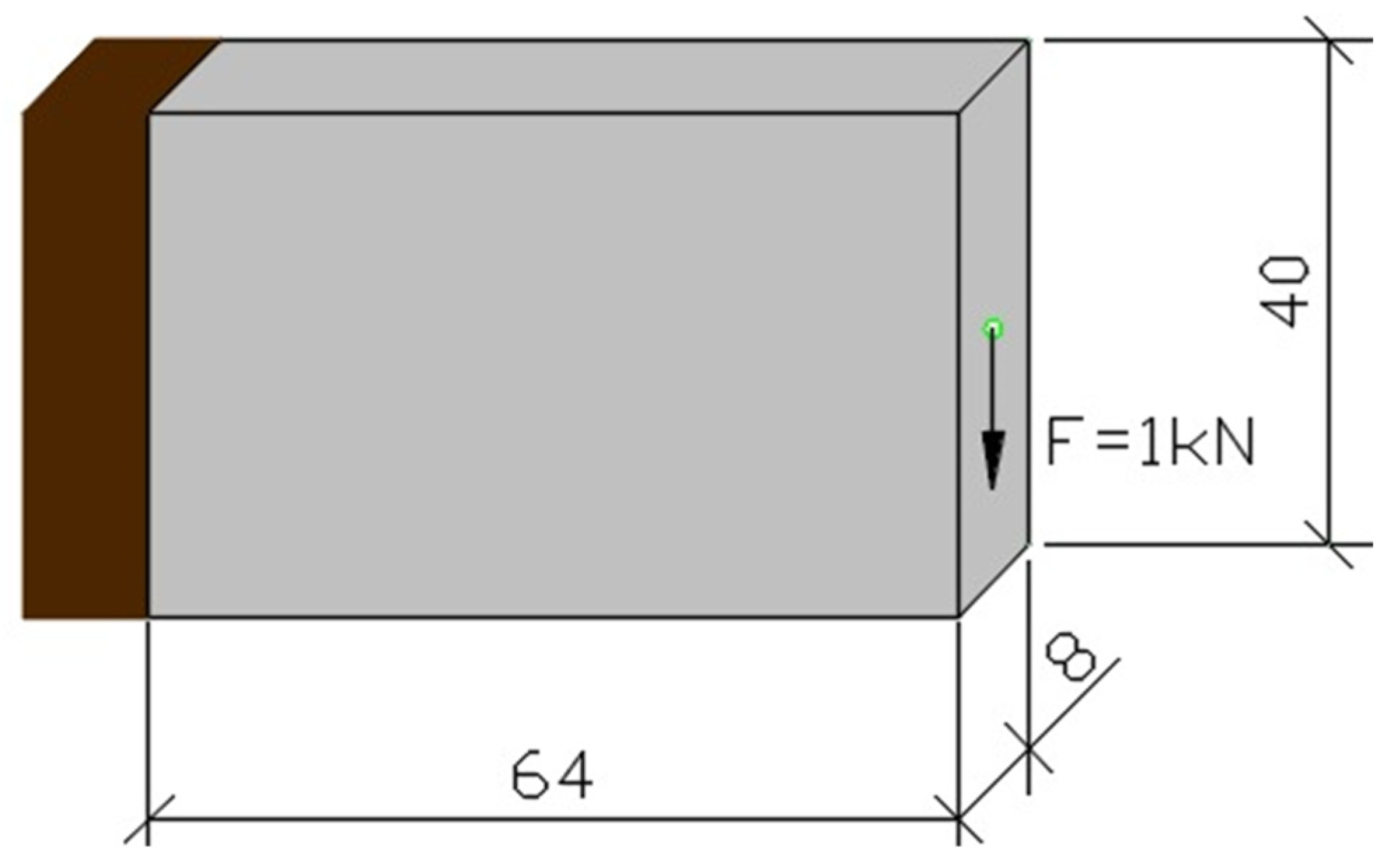
4.1. Cantilever Beam

This classic example from the literature is presented to validate the formulation presented in this article. The design domain, boundary conditions, and optimal topologies of a cantilever beam with a single, isotropic material are shown in Figure 2 and Figure 3. In Figure 3a, the cantilever is optimized using the BESO method, while Figure 3b shows the same cantilever optimized using the SESO method. The material properties are Young’s modulus E = 1 MPa and Poisson’s ratio μ = 0.3. The design domain and boundary conditions are displayed in Figure 2. The left end is fixed, and a concentrated load F = 1 kN is applied at the center of the free face. The optimization parameters used are prescribed volume fraction ${\mathbf{V}}_{\mathbf{f}}=0.20$ and filter radius $\mathbf{r}=1.5\mathrm{m}\mathrm{m}.$ The design domain is discretized into a 64 × 40 × 8 element mesh, totaling 20,480 hexahedral finite elements with 1 mm edge lengths.

The optimization procedure with the BESO method was carried out with an evolutionary ratio $ER=0.03$ with a computational cost of 47.8 min and compliance of 11.3334 N × mm. While in the SESO method, a rejection ratio $RR=0.01$ and an $ER=0.02$ were used with a computational cost of 32.5 min and compliance of 11.5428 N × mm. It can be seen that the upper part of the cantilever is in tension (blue color) while the lower part is compressed.

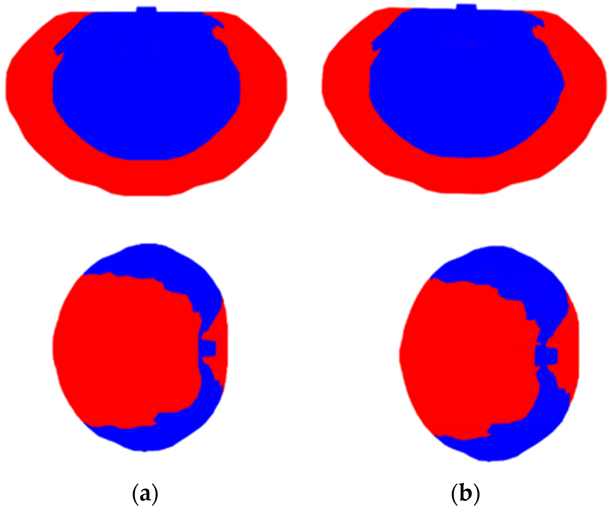
4.2. Example 2—Application of BESO and SESO to the Design of an Apple

One of the most intriguing questions about nature and structures that evolve naturally is “What is the reason for them to have the optimal configuration they do?” To answer this question and validate the implementation of the structure’s self-weight, the evolutionary optimization methods BESO and SESO, for three-dimensional structures, are applied in a natural optimization design. Figure 4 presents the design domain and boundary conditions of a structure that will only be subjected to the action of its weight. Thus, it would be possible to verify whether these methods could reproduce the same shape of an apple created by nature in order to determine whether its appearance was influenced by a genetic or structural perspective.

The design domain was subdivided using 8-node hexahedral elements, as proposed by [25], with dimensions of 1 × 1 × 1 mm. The applied load consists of a downward acceleration of 1 g, equivalent to −9.8 m/s². The assumed density for all elements was 2700 kg/m³, and the modulus of elasticity of the material was assumed to be 70 × 10³ MPa, as proposed by [10]. The prescribed final volume is $V_f=0.30$ and the filter radius is $r=2 \mathrm{m}\mathrm{m}$. The design domain illustrated in Figure 4 has 10,543 hexahedral finite elements. In the evolutionary optimization procedure, the evolutionary ratio used in BESO was $ER=0.03$, while in SESO $RR=0.01$ and $ER=0.02$ were considered. Poisson’s ratio was equal to 0.30. Figure 5 illustrates that the optimal configurations obtained by the methods presented in this article resemble the shape of a fruit, specifically that of an apple. This result is notable, as the final topology was achieved exclusively through structural constraints. This suggests that, at least for this domain, the final form was predominantly developed from a structural perspective rather than biological reasons.

In Figure 5, it is observed that both by the BESO method, Figure 5a,b, and by the SESO method, Figure 5, the influence of self-weight results in traction in the structure. This effect causes tension in the elements located close to the center of gravity, evidenced by the blue color. On the other hand, the elements closest to the ends of the structure are subject to compression, indicated by the color red.

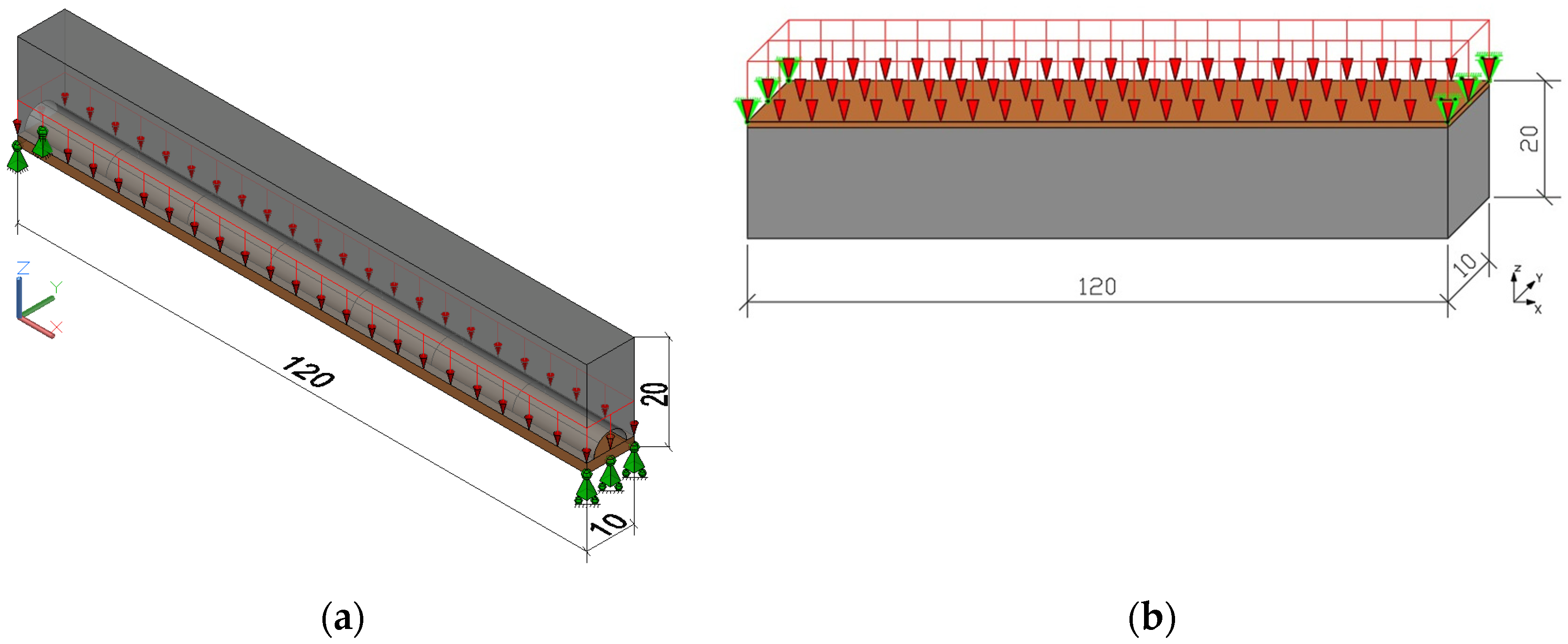
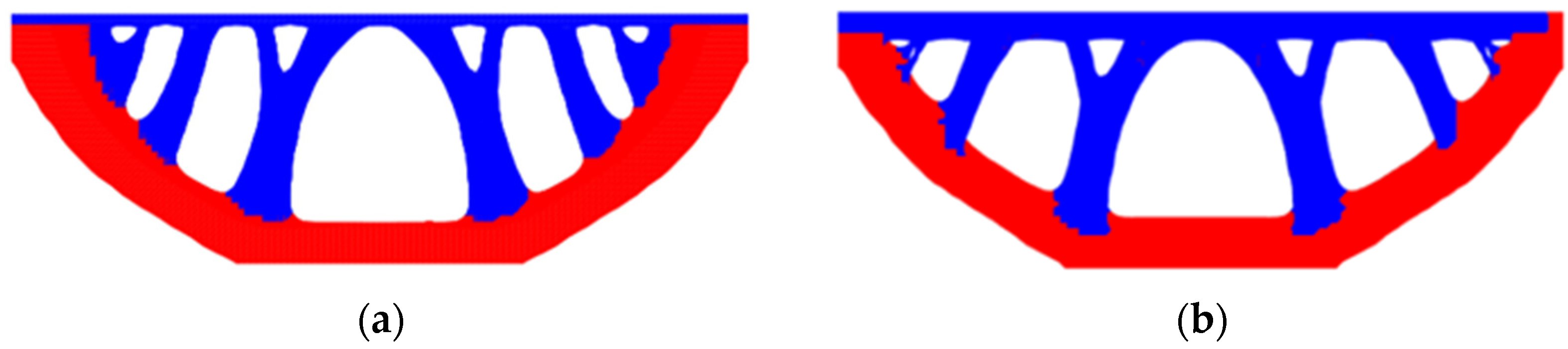
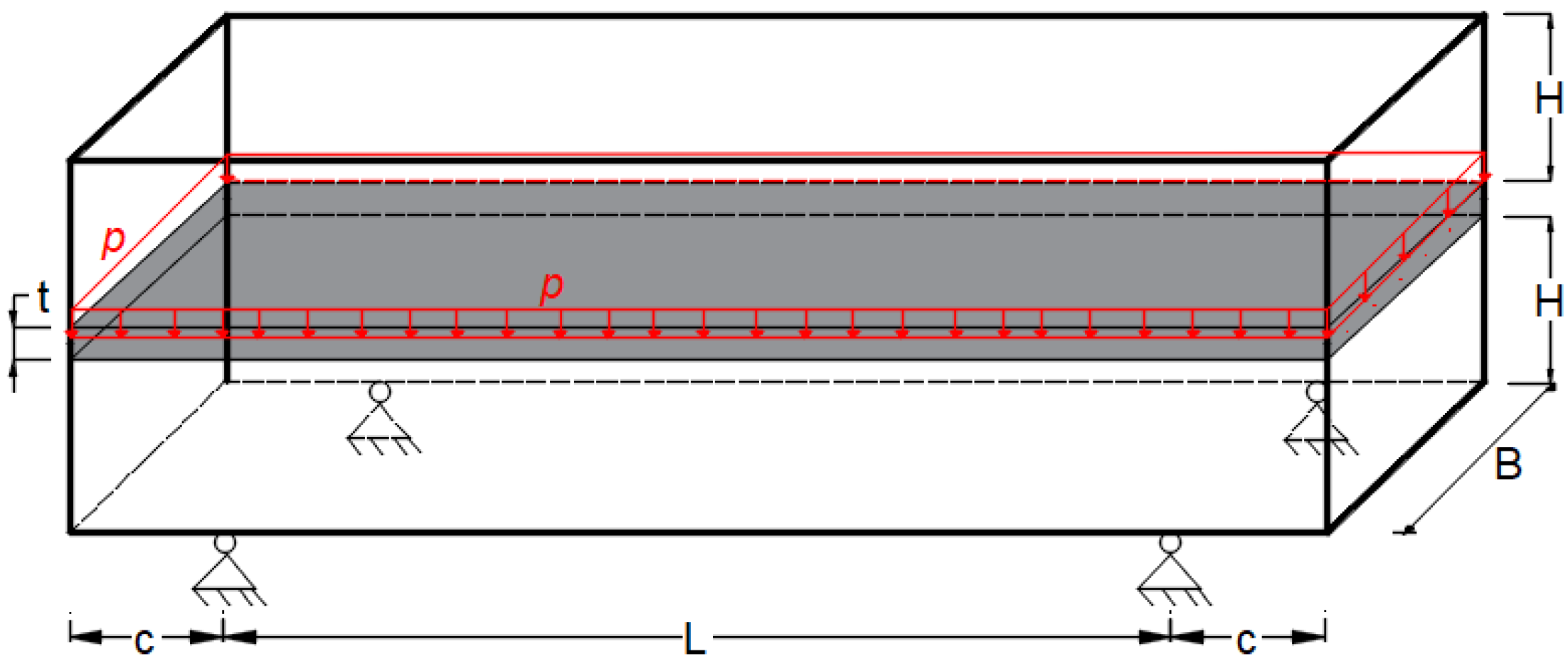
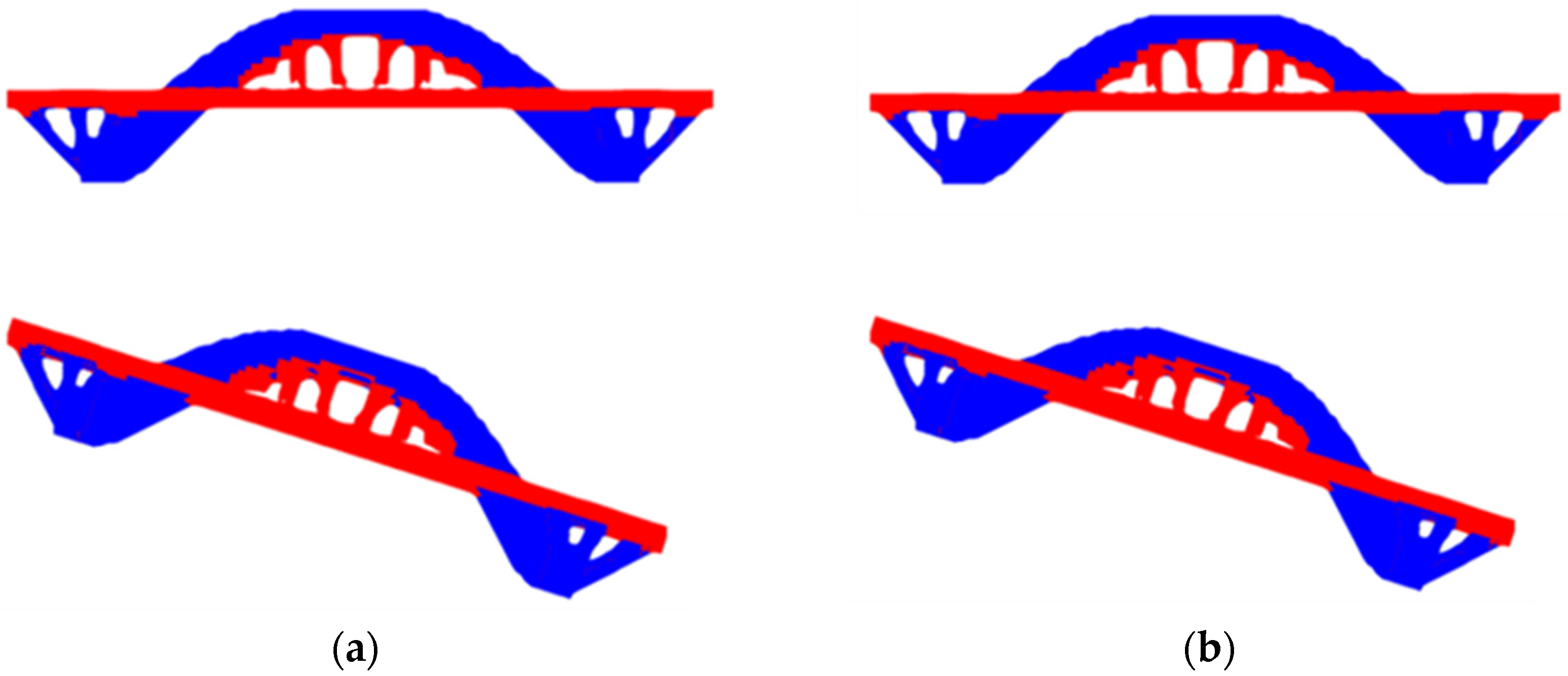
4.3. Example 3—Deterministic Analysis: Bridge Topology Optimization

The optimization procedure via BESO and SESO methods will be carried out for the examples of bridges shown in Figure 6a,b with a span of 120 m, a width of 10 m, and a height of 20 m. In Figure 6a, there is a bridge with a lower deck designed with a semicircular space in the x direction intended for traffic and will be considered a non-design domain. The lower left end of the board is fixed in all directions, while the right end allows movement in the x direction. The bridge illustrated in Figure 6b has an upper deck with the left end fixed in the x, y, and z directions, while the right end allows movement in the x direction. The load used in both designs is uniformly distributed with $F=1\times {10}^5 \mathrm{N}/{\mathrm{m}}^2.$ The prescribed final volume is $V_f=0.30$ and the filter radius is $r=3 \mathrm{m}$. The board is defined as a non-design domain region. In the evolutionary optimization procedure, the evolutionary ratio used in BESO was $ER=0.03$, while in SESO, $RR=0.01$ and $ER=0.02$ were considered.

In case (a), a bridge that has a hole in the x direction, the optimized structure resembles tied arch bridges, with concrete (blue color) shaping the arch above the deck, while steel is used in the tie rods and the deck (red), as seen in Figure 7a,b. Aesthetically, the cables take the form of catenaries due to the influence of gravity. In contrast, case (b), as seen in Figure 8a,b, presents a substantially different configuration, with the majority of the structure located below the bridge deck, as proposed by [31]. In this situation, an arch in the opposite direction to that in case (a) is formed, with the steel playing the main role by composing a brace that supports the main load of the bridge. Concrete, in turn, is used to build the deck and the small inclined columns that connect the deck to the belt. However, it is possible to observe that BESO presents a topology with the internal arc above the deck that is clearer than SESO, which presents a topology in the shape of two oblique cables.

In case (b), the deterministic optimal topologies presented in Figure 8a,b, the presence of regions that transmit efforts (blue) and regions that are compressed (red) is evident. In this article, allowable stress values for tension and compression were incorporated, and, in the case of rods subjected to compression, it is essential to consider the possibility of failures due to buckling (slenderness) when sizing the designs.

4.4. Example 4—Reliability-Based Topology Optimization without Considering Self-Weight

The optimization process in the example in Section 4.3 was developed based on the reliability analysis proposed by [30]. In this example, geometry, volume, modulus of elasticity, and compliance obtained from the deterministic analysis were considered as random variables. Coupling structural reliability analysis into the BESO-3D and SESO-3D methods demonstrated effectiveness and robustness when optimizing the bridges illustrated in Figure 6a,b. It is worth mentioning that the optimal configurations obtained are as slender as the previous ones, without significant differences in terms of structural design. For this analysis, a target reliability index ${\beta }_t=3.0$ was considered, which is equivalent to a probability of structure failure equal to $P_f=0.001358$.

The initial design parameters are presented in

Table 1. Coefficients in constitutive relations.

Distribution Parameter	Distribution Type	Mean ($\mathit{\mu }$)	Standard Deviation ($\mathit{\sigma }$)
nelx (mm)	Normal	120	0.1
nely (mm)	Normal	20	0.1
nelz (mm)	Normal	10	0.1
E (GPa)	Normal	1	0.1
$\mathit{\nu }$	Constant	0.30	0
F (1000 N/m2)	Normal	1	0.1
Volume (mm3)	Normal	0.30	0.1
Compliance (N.mm)	Normal	4.82 × 106	0.1

, where nelx (length), nely (height), and nelz (width) represent the geometry of the structure, F represents the distributed external load, E represents the modulus of elasticity, V represents the volume of the structure, and C represents compliance and are considered random variables with normal distribution, while Poisson’s ratio (ν) has a constant distribution.

Figure 9a,b illustrates, respectively, the optimal configurations obtained by the two methods presented in this article. It is noteworthy that both BESO and SESO converged with three FORM iterations and 81 topology iterations with computational costs, respectively, equal to 73.02 min and 50.41 min. It is noteworthy that the computational performance of SESO for all examples presented in this article is superior to BESO.

It is observed that the optimal configuration for both methods is equivalent. It is noteworthy that BESO has a configuration closer to SESO when considering the reliability analysis of the structure; the arc presented in Figure 6a tends here for inclined cables. It is noteworthy that the allowable stress used as a constraint in the examples is derived from the Deterministic Topology Optimization (DTO) procedure. The problem is initially solved using DTO, and the resulting von Mises stress from this optimization is utilized as the permissible stress. In this example, the value of ${\sigma }^{\ast }=153.84 \mathrm{N}\times \mathrm{m}$.

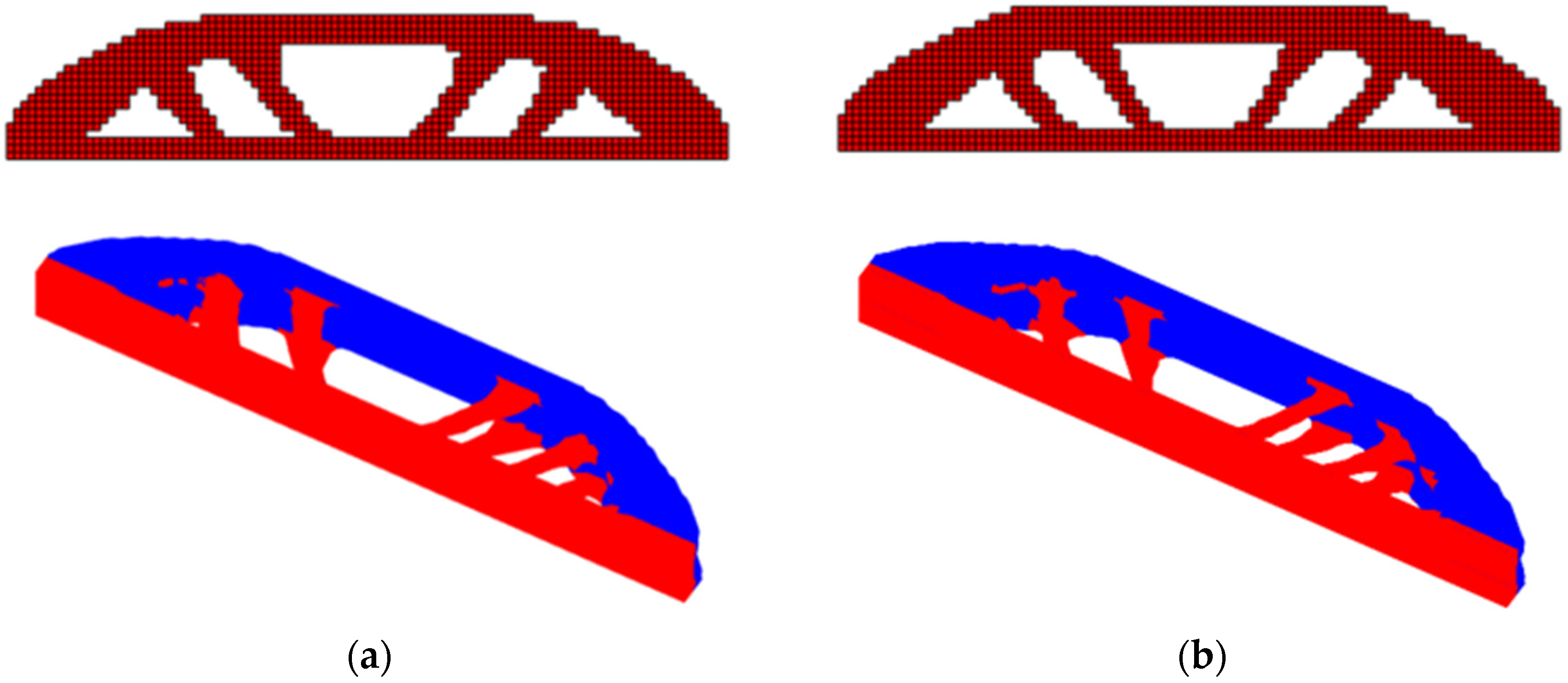
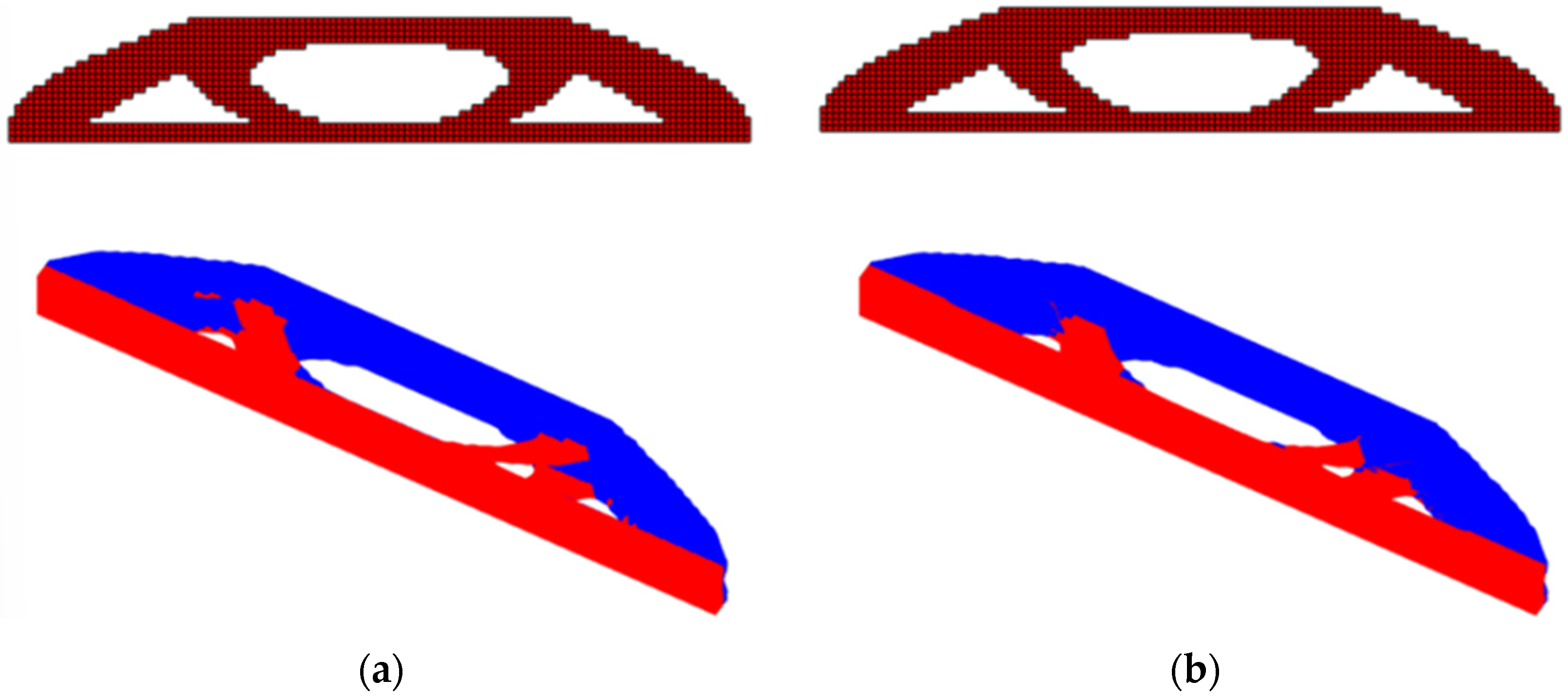
4.5. Example 5—Reliability-Based Topology Optimization Considering Self-Weight

The bridge shown in Figure 6a was analyzed by coupling the structure’s own weight in the optimization procedure with the aim of analyzing the influence of the self-weight on the optimal configuration. It is worth mentioning that the optimal configurations obtained by the RBTO-BESO_3D and RBTO-SESO_3D methods are different in terms of structural design. However, when examining the optimal configurations, considering the self-weight, as seen in Figure 10, we observed that the two models produced similar configurations with just a denser arc in the shape of a catenary. These changes in topology are attributable to the influence of gravitational force and have important implications for engineers. This is due to the fact that optimizing the structure while taking into account its self-weight can result in more efficient and safe solutions.

4.6. Example 6—Reliability Analysis—Effects of Boundary Conditions and Self-Weight on Bridge Topology

Figure 11 displays the design domain and boundary conditions of a bridge with three different support locations. The objective is to analyze the influence of the location of the supports on the optimal configuration for different reliability indices. Furthermore, we consider geometry, volume, loading, compliance, and elastic modulus as random variables with a normal distribution and a standard deviation equal to 0.1. In this study, we consider the self-weight of the structure during the optimization process. The material density was defined for a steel structure: $\mathsf{\rho }=7800\mathrm{k}\mathrm{g}/{\mathrm{m}}^3$. The volume fraction is set to $V=0.25$ and the filter radius is set to $r=1.5 \mathrm{m}$. In each case, the mesh is defined as 120 × 30 × 10, totaling 36,000 hexahedral finite elements with eight nodes according to Liu et al. (2014). The deck with a thickness $\mathrm{t}=1.0 \mathrm{m}$ is defined as a non-design domain area shown as the darker area in Figure 11, and $H=14.5 \mathrm{m}$, $L=90 \mathrm{m}$, $c=15 \mathrm{m}$, and $B=10.0 \mathrm{m}.$ Therefore, the region in the highlighted region will not be allowed to remove solid elements.

Figure 12 displays the deterministic optimal topologies obtained by the two methods covered in this article. Although the topologies are identical, the SESO method required a computational cost of 1.5 h, resulting in a compliance of $\mathrm{C}=6.479\times {10}^5\mathrm{N}.\mathrm{m}$, while the BESO method required $\mathrm{t}\mathrm{i}\mathrm{m}\mathrm{e}=1.6$ h of computational cost and resulted in a compliance of $\mathrm{C}=6.495\times {10}^5\mathrm{N}.\mathrm{m}$.

In the optimal configurations shown in the Figure 13a BESO and Figure 13b SESO, reliability analysis was considered with an equal reliability index ${\beta }_t=3$, but the structure’s weight was not considered. It is noted that the topologies are similar, with a final volume 15% smaller than in deterministic topologies and computational costs 8% lower for SESO. It is worth mentioning that the compliance presented by BESO is 0.2% lower than in SESO. Additionally, SESO introduced more tensile cables on tensile arch bridges to help support the bridge load and distribute it effectively. In a tensile arch bridge, the arch supports most of the load through compression, but the tensile cables help distribute some of this load laterally to the supporting piers and ends of the bridge. These tensile cables help to stabilize the bridge structure and prevent excessive deformation under load, thus ensuring the safety and stability of the bridge.

The example represented in Figure 11 was analyzed for different reliability indices, as shown in

Table 2. Influence of the reliability index ${\beta }_t$ on Topology Optimization.

Opt. Techniques	RBTO-BESO	RBTO-SESO	Time RBTO-BESO (Hours)/Compliance/Iteration FORM	Time RBTO-SESO (Hours)/Compliance/Iteration FORM
${\mathit{\beta }}_{\mathit{t}}=1$			Time = 2.22 $C=3.58\times {10}^7$ $iter=1$	Time = 1.86 $C=3.68\times {10}^7$ $iter=1$
${\mathit{\beta }}_{\mathit{t}}=2$			Time = 1.62 $C=2.61\times {10}^7$ $iter=3$	Time = 1.33 $C=2.77\times {10}^7$ $iter=3$
${\mathit{\beta }}_{\mathit{t}}=3$			Time = 1.37 $C=2.53\times {10}^7$ $iter=4$	Time = 1.19 $C=2.71\times {10}^7$ $iter=4$
${\mathit{\beta }}_{\mathit{t}}=4$			Time = 1.56 $C=2.45\times {10}^7$ $iter=6$	Time = 1.24 $C=2.67\times {10}^7$ $iter=6$
${\mathit{\beta }}_{\mathit{t}}=5$			Time = 1.58 $C=2.29\times {10}^7$ $iter=8$	Time = 1.25 $C=2.57\times {10}^7$ $iter=8$
${\mathit{\beta }}_{\mathit{t}}=6$			Time = 1.83 $C=2.15\times {10}^7$ $iter=9$	Time = 1.25 $C=2.38\times {10}^7$ $iter=9$

, for the two methods proposed in this article. The random variables follow the data in Table 1. It is noteworthy that the RBTO models provided a volume reduction in relation to the DTO models of approximately 9%. It can be seen that the optimal topologies presented while considering the structure’s weight are different from the deterministic optimal topologies without considering the self-weight. This is because the tensile arch is mainly responsible for supporting compression loads, while the bridge deck, which is under compression, is responsible for transmitting these loads to the supports. In this case, cables are not needed because the loads are being transferred directly through the arch and deck without the need for an additional tensile cable structure.

When considering the structure’s self-weight, a fully distributed load and the influence of gravity throughout the analyzed domain are taken into account. Therefore, it results in lighter and more efficient structures, as expected, according to [32].

The computational cost of SESO is significantly lower than that of BESO. However, BESO achieves lower compliance for the analyzed reliability indices. This behavior is illustrated in Figure 14 which also demonstrates that as the level of reliability increases (i.e., as the value of β increases), the stiffness of the structure decreases, as predicted by [30]). Furthermore, an increase in β, with the same boundary conditions, geometry, and random variables, does not significantly alter the optimal configurations, as shown in Table 2. Under these conditions, what changes is the solution of the problem known as the design point P*, as illustrated in Figure 15.

One approach to identify a good approximation point is to first transform the original random variable space into an independent Gaussian space. Then, the Most Probable Point (MPP) is identified as the approximation point for the g-function, as illustrated in Figure 15. In the transformed u-space, the MPP is the point of minimum distance from the origin to the g = 0 surface. This minimum distance β is called the reliability index, and in the FORM, the solution is usually referring to a linear approximation in the u-space, and it can show that the corresponding exact $P_f$ is given by

$$P_f=\mathsf{\Phi }(-\beta )$$

(11)

5. Conclusions

This article presents a qualitative comparison between the BESO and SESO methods, revealing that both are effective in generating optimal topologies for three-dimensional structural systems, considering compliance minimization and the influence of the structure’s self-weight. The analyzed examples demonstrate that these methods produce configurations that meet structural efficiency requirements, remaining robust even in the face of variations in boundary conditions and design parameters. Furthermore, the incorporation of the structure’s self-weight into both methods, along with reliability analyses, represents a significant contribution to the field of optimal topology for structural systems. Notably, SESO exhibits a lower computational cost in all examples, while BESO results in lower compliance. These approaches provide engineers with an advanced and reliable tool for the automated design of structures by distinguishing between tensile (blue) and compression (red) regions, ensuring greater efficiency in practical applications.

During the investigation, it was found that the sensitivity of the von Mises stress derivatives with respect to the x and z directions produces results similar to those presented in the literature for tensile and compression states that use principal stresses. However, the authors are developing a mathematical and geometric relationship to demonstrate this correspondence for a future publication.

References

1. Svanberg, K. Method of moving asymptotes—A new method for structural optimization. Int. J. Num. Meth. Eng. 1987, 24, 359–373. [Google Scholar] [CrossRef]
2. Bendsøe, M.P. Optimal shape design as a material distribution problem. Struct. Optim. 1989, 1, 193–202. [Google Scholar] [CrossRef]
3. Zhou, M.; Rozvany, G.I.N. The COC algorithm, Part II: Topological, geometrical and generalized shape optimization. Comp. Meth. Appl. Mech. Engrg. 1991, 89, 309–330. [Google Scholar] [CrossRef]
4. Eschenauer, H.A.; Kobelev, V.V.; Schumacher, A. Bubble method for topology and shape optimization of structures. Struct. Optim. 1994, 8, 42–51. [Google Scholar] [CrossRef]
5. Allaire, G.; Jouve, F.; Toader, A.-M. A level set method for shape optimization. C. R. Acad. Sci. Paris Série I 2002, 334, 1125–1130. [Google Scholar] [CrossRef]
6. Wang, M.Y.; Wang, X.; Guo, D. A level set method for structural topology optimization. Comput. Methods Appl. Mech. Engrg. 2003, 192, 227–246. [Google Scholar] [CrossRef]
7. Xia, Q.; Shi, T. Topology optimization of compliant mechanism and its support through a level set method. Comput. Methods Appl. Mech. Eng. 2016, 305, 359–375. [Google Scholar] [CrossRef]
8. Xie, Y.M.; Steven, G.P. Um procedimento evolucionário simples para otimização estrutural. Comput. Estrut. 1993, 49, 885–896. [Google Scholar] [CrossRef]
9. Xie, Y.M.; Steven, G.P. Evolutionary Structural Optimization; Springer: Berlin/Heidelberg, Germany, 1997. [Google Scholar] [CrossRef]
10. Querin, O.M.; Steven, G.P.; Xie, Y.M. Evolutionary structural optimisation (ESO) using a bidirectional algorithm. Eng. Comput. 1998, 15, 1031–1048. [Google Scholar] [CrossRef]
11. Yang, X.Y.; Xie, Y.M.; Steven, G.P.; Querin, O.M. Topology optimization for frequencies using an evolutionary method. J. Struct. Eng. 1999, 125, 1432–1438. [Google Scholar] [CrossRef]
12. Querin, O.M.; Young, V.; Steven, G.P.; Xie, Y.M. Computational efficiency and validation of bi-directional evolutionary structural optimisation. Comput. Methods Appl. Mech. Eng. 2000, 189, 559–573. [Google Scholar] [CrossRef]
13. Huang, X.; Xie, Y.M.; Burry, M.C. Advantages of bi-directional evolutionary structural optimization (BESO) over evolutionary structural optimization (ESO). Adv. Struct. Eng. 2007, 10, 727–737. [Google Scholar] [CrossRef]
14. Almeida, V.S.; Simonetti, H.L.; Neto, L.O. Comparative analysis of strut-and-tie models using Smooth Evolutionary Structural Optimization. Eng. Struct. 2013, 56, 1665–1675. [Google Scholar] [CrossRef]
15. Simonetti, H.L.; Almeida, V.S.; de Oliveira Neto, L. A smooth evolutionary structural optimization procedure applied to plane stress problem. Eng. Struct. 2014, 75, 248–258. [Google Scholar] [CrossRef]
16. Shobeiri, V.; Ahmadi-Nedushan, B. Bi-directional evolutionary structural optimization for strut-and-tie modelling of three-dimensional structural concrete. Eng. Optim. 2017, 49, 2055–2078. [Google Scholar] [CrossRef]
17. Shobeiri, V. Determination of strut-and-tie models for structural concrete under dynamic loads. Can. J. Civ. Eng. 2019, 46, 1090–1102. [Google Scholar] [CrossRef]
18. Huang, X.; Zuo, Z.H.; Xie, Y.M. Evolutionary topological optimization of vibrating continuum structures for natural frequencies. Comput. Struct. 2010, 88, 357–364. [Google Scholar] [CrossRef]
19. Zuo, Z.H.; Xie, Y.M. A simple and compact Python code for complex 3D topology optimization. Adv. Eng. Softw. 2015, 85, 1–11. [Google Scholar] [CrossRef]
20. Bi, M.; Tran, P.; Xie, Y.M. Topology optimization of 3D continuum structures under geometric self-supporting constraint. Addit. Manuf. 2020, 36, 101422. [Google Scholar] [CrossRef]
21. Habashneh, M.; Movahedi Rad, M. Reliability based geometrically nonlinear bi-directional evolutionary structural optimization of elasto-plastic material. Sci. Rep. 2022, 12, 5989. [Google Scholar] [CrossRef]
22. Eom, Y.S.; Yoo, K.S.; Park, J.Y.; Han, S.Y. Reliability-based topology optimization using a standard response surface method for three-dimensional structures. Struct. Multidiscip. Optim. 2011, 43, 287–295. [Google Scholar] [CrossRef]
23. Simonetti, H.L.; Almeida, V.S.; de Assis das Neves, F.; Del Duca Almeida, V.; de Oliveira Neto, L. Reliability-Based Topology Optimization: An Extension of the SESO and SERA Methods for Three-Dimensional Structures. Appl. Sci. 2022, 12, 4220. [Google Scholar] [CrossRef]
24. Simonetti, H.L.; Almeida, V.S.; Neves FdAd Almeida, V.D.D.; Cutrim, M.D.S. 3D Structural Topology Optimization Using ESO, SESO and SERA: Comparison and an Extension to Flexible Mechanisms. Appl. Sci. 2023, 13, 6215. [Google Scholar] [CrossRef]
25. Liu, K.; Tovar, A. An efficient 3D topology optimization code written in Matlab. Struct. Multidiscip. Optim. 2014, 50, 1175–1196. [Google Scholar] [CrossRef]
26. Han, Y.; Xu, B.; Wang, Q.; Liu, Y. Bi-directional evolutionary topology optimization of continuum structures subjected to inertial loads. Adv. Eng. Softw. 2021, 155, 102897. [Google Scholar] [CrossRef]
27. Meng, D.; Yang, H.; Yang, S.H.; Zhang, Y.; Jesus, A.M.; Correia, J.; Fazeres-Ferradosa, T.; Macek, W.; Branco, R.; Zhu, S. Kriging-assisted hybrid reliability design and optimization of offshore wind turbine support structure based on a portfolio allocation strategy. Ocean. Eng. 2024, 295, 116842. [Google Scholar] [CrossRef]
28. Meng, D.; Yang, S.; Yang, H.; De Jesus, A.M.; Correia, J.; Zhu, S.P. Intelligent-inspired framework for fatigue reliability evaluation of offshore wind turbine support structures under hybrid uncertainty. Ocean. Eng. 2024, 307, 118213. [Google Scholar] [CrossRef]
29. Yang, S.; Meng, D.; Wang, H.; Yang, C. A novel learning function for adaptive surrogate-model-based reliability evaluation. Philos. Trans. R. Soc. A 2024, 382, 20220395. [Google Scholar] [CrossRef]
30. Kharmanda, G.; Olhoff, N.; Mohamed, A.; Lemaire, M. Reliability-based topology optimization. Struct. Multidiscip. Optim. 2004, 26, 295–307. [Google Scholar] [CrossRef]
31. Li, Y.; Yuan, P.F.; Xie, Y.M. A strategy for improving the safety and strength of topologically optimized multi-material structures. Acta Mech. Sin. 2023, 39, 422134. [Google Scholar] [CrossRef]
32. Jain, N.; Saxena, R. Effect of self-weight on topological optimization of static loading structures. Alex. Eng. J. 2018, 57, 527–535. [Google Scholar] [CrossRef]
Figure 1. SESO Flowchart with own weight.
Applsci 14 06465 g001
Figure 2. Design domain and boundary conditions.
Applsci 14 06465 g002
Figure 3. Optimal topologies: (a) BESO and SESO principal stresses and (b) BESO and SESO Sensitivity Analysis.
Applsci 14 06465 g003aApplsci 14 06465 g003b
Figure 4. Design domain and boundary conditions.
Applsci 14 06465 g004
Figure 5. Optimal topologies: (a) SESO and (b) BESO.
Applsci 14 06465 g005
Figure 6. Design domain and boundary conditions: (a) Bridge with lower deck and semicircular opening in the x direction and (b) bridge with upper deck.
Applsci 14 06465 g006
Figure 7. Deterministic optimal topologies: (a) BESO and (b) SESO.
Applsci 14 06465 g007
Figure 8. Deterministic optimal topologies: (a) BESO and (b) SESO.
Applsci 14 06465 g008
Figure 9. RBTO: (a) BESO and (b) SESO.
Applsci 14 06465 g009
Figure 10. RBTO with own weight: (a) BESO and (b) SESO.
Applsci 14 06465 g010
Figure 11. Design domain and boundary conditions.
Applsci 14 06465 g011
Figure 12. Deterministic procedure topology optimization: (a) BESO and (b) SESO.
Applsci 14 06465 g012
Figure 13. RBTO considering self-weight: (a) BESO and (b) SESO.
Applsci 14 06465 g013
Figure 14. Graph—objective function by reliability index.
Applsci 14 06465 g014
Figure 15. The P*: Ideal g-function approximation point.
Applsci 14 06465 g015