Article

The Electrical Characteristics Generated by Resetting the Particle Organization Configuration of Rocks under Compressive Loads

1
School of Architecture and Transportation Engineering, Guilin University of Electronic Technology, Guilin 541004, China
2
Guangxi Key Laboratory of ITS, Guilin University of Electronic Technology, Guilin 541004, China
3
School of Computer Science and Information Security, Guilin University of Electronic Technology, Guilin 541004, China
4
Beihai Product Quality Testing Institute, Beihai 536000, China
*
Author to whom correspondence should be addressed.
Appl. Sci. 2024, 14(15), 6474; https://doi.org/10.3390/app14156474
Submission received: 7 July 2024 / Revised: 21 July 2024 / Accepted: 21 July 2024 / Published: 25 July 2024
(This article belongs to the Section Civil Engineering)

Abstract

:
Under compressive loading, rocks emit electromagnetic waves, and monitoring electromagnetic signals has become a key means of predicting dynamic rock disasters. To understand how dynamic potential is generated in rocks under compressive loading, the relationship between the compressive loading (P) and the stimulated potential (E) is seen as a circuit system (H(t)). A circuit analysis model has been established to study how rock particles restructure under compressive loading. Experimental tests were conducted to measure the input excitation (E) and output response (Uσ(t)) or (Iσ(t)) of the rock specimens, with four types of rocks being tested. The experiments revealed that voltage, current, frequency, and impedance changed during the particle reorganization process under compressive loading, showing that the electromagnetic radiation of the rock specimens mainly came from the current generated by the internal particle reorganization. The intensity of electromagnetic radiation was found to depend on the load size and dynamic impedance (Zσ), with the dynamic impedance (Zσ) consisting of the microelement total resistance (Rσ), capacitance (Cσ), and inductance (Lσ). The variation of dynamic impedance (Zσ) is related to the rock type. The research findings have contributed to elucidating the mechanism of electromagnetic radiation generated by rocks under load.

1. Introduction

In the design, construction, operation, and maintenance of tunnel, subgrade, rock slope, and mining projects, it is often necessary to fully utilize the compressive properties of rocks [1,2]. In-depth research on the mechanical laws and response characteristics of rocks under compressive loading is particularly crucial for averting geological disasters. Rocks exhibit nonlinear stress and strain changes and generate various physical signals when subjected to external compressive load [3,4,5,6,7]. By utilizing these physical signals to obtain dynamic precursor information of rock failure, geological disasters can be predicted, and the impact of geological disasters can be minimized to the greatest extent [8,9,10,11]. When rocks undergo changing compressive stress, free charges move and generate electromagnetic signals. The advantage of electromagnetic signals is their fast propagation speed, which makes the electromagnetic signal monitoring method a key means of predicting dynamic rock disasters [12].
To take advantage of the electromagnetic signals emitted by rocks under pressure, scholars began to explore the laws of these signals as rocks are subjected to external compressive loads. In the early stage, Brady et al. [13], Cress et al. [14], and Fukui et al. [15], respectively, reported the electromagnetic radiation (EMR) events of rock under external compression loads. Hajjcontis and Mavromatou [16] observed the changes in the electric field before complete failure of rock under uniaxial loading conditions with different strain rates. Yoshida et al. [17] detected EMR signals during granite fracture failure, and Rabinovitch et al. [18] confirmed that rocks radiate electromagnetic signals in a certain area before and after peak stress. In addition, Carpinteri et al. [19] also studied the acoustic emission (AE) and EMR characteristics of concrete and rock samples during laboratory compression tests, and verified that AE and EMR signals are the precursors of concrete and rock collapse. Yamada et al. [20] conducted experiments to record the electromagnetic radiation (EMR) and acoustic emission (AE) signals of granite samples under constant strain rate loading, finding that the onset time of EMR coincided with that of AE, and concluding that electromagnetic wave emissions were associated with microcracks in the samples. Frid et al. [21] noted that as cracks continued to propagate, EMR amplitude increased; when crack propagation ceased, EMR pulse amplitude decayed. Frid et al. [22] investigated a new technique for detecting high-frequency EMR signals emitted by rock microcracks to anticipate the initial stage of mine roof collapse. When analyzing the example results of EMR and low-frequency AE before the roof collapse in Moonee Colliery, it was found that abnormally high EMR was detected more than 1 h before the roof collapse, which had a significant time advantage compared with the first indicator of low-frequency AE. Qiu et al. [23] conducted tests on coal rocks to analyze the characteristics of low-frequency electromagnetic radiation signals (1 kHz) during sample fracture failure, and theoretically established the relationship between EMR signals and staged fractures. The above research confirms that rocks emit electromagnetic signals when subjected to pressure, and these signals are closely associated with the progression of rock damage. However, the mechanism of electromagnetic radiation from compressed rocks remains a perplexing issue.
Scholars have made great efforts to explore the underlying mechanisms behind the electromagnetic radiation emitted by rocks under the action of external compressive loading. Ogawa et al. [24] discovered the phenomenon of granite emitting electromagnetic waves in 1985 and discussed the process of generating electric dipole moments from the perspectives of contact electrification and piezoelectric electrification. Song et al. [25] performed three-point bending tests on rock samples with notches using real-time resistivity and acoustic emission testing technology, revealing changes in overall potential distribution characteristics due to crack initiation and propagation, which affected overall resistivity. Baddari et al. [26] investigated the rock loading process and observed that the non-uniform distribution of the spatial crystal structure of the rock resulted in variations in EMR and AE characteristics. They also noted that different stress levels led to distinct rock EMR and AE behaviors upon failure. Han et al. [27] conducted an experimental study on the EMR characteristics of rocks at various degrees of damage, and highlighted the influence of electric dipoles generated during different stages of crack propagation on the spectrum and amplitude changes of the EMR signal. Wei et al. [28] concluded that quartz content was not a determining factor for the strength of the EMR signal, but rather it was influenced by complex crack events induced by stress during loading. Li et al. [29] derived a theoretical model of loaded composite coal rocks with cracks, conducted uniaxial compression tests on composite coal rocks, and studied the influence of coal rock crack state on the time–frequency characteristics of EMR signals.
Xiao et al. [30] analyzed the measurement results of EMR and AE signals emitted by coal under uniaxial compression, and concluded that the research on the relationship between the electromagnetic radiation intensity and stress in the process of coal damage and failure can be carried out based on the idea of energy conversion. Nie et al. [31] proposed an electromechanical coupling model for coal under compression load, integrating strength statistical theory and damage mechanics theory, and indicated that electromagnetic radiation can characterize the damage stage of coal under compression load. Li et al. [32] carried out experimental research on electric potential (EP) signals from four types of samples under compression load, analyzed the EP response characteristics at different loading stages, and highlighted crack propagation as a significant mechanism in EP response, including electron escape due to stress concentration at the crack tip, charge separation caused by crack propagation, and discharge at the crack tip. Triantis et al. [33] and Wan et al. [34] discussed the temporal evolution of electrical activity in brittle materials and compared it with acoustic emission technology test results, revealing common qualitative characteristics among these sensing technologies.
Therefore, the electromagnetic signals generated by rocks under load can be used as characteristic information for predicting rock fracture and failure. There are many complex analytical models for the electromagnetic radiation of rock deformation and failure, and the dominant factors for different degrees of rock deformation and failure are different. In other words, there is no unified understanding of the cause of rock electromagnetic radiation. From the perspective of electromagnetics, the electromagnetic signals generated by rocks under pressure can take the form of direct current (DC), alternating current (AC), or non-periodic signals.
In order to establish a unified interpretation model, this paper starts from the perspective of resetting the particle organization structure of rocks, and establishes a unified analytical model for generating direct current, alternating current, and non-periodic electromagnetic signals in the deformation and failure process of rock materials. Based on the structure of the pressure machine and the physical properties of rocks, the response of the test piece under load and deformation and failure is regarded as an independent system, and the response pattern is solved by system excitation, establishing a multi-cause circuit analysis model that includes inductance (L), capacitance (C), and resistance (R) to reveal the electrical characteristics caused by the reset of the particle organization structure of rocks under pressure.

2. Materials and Methods

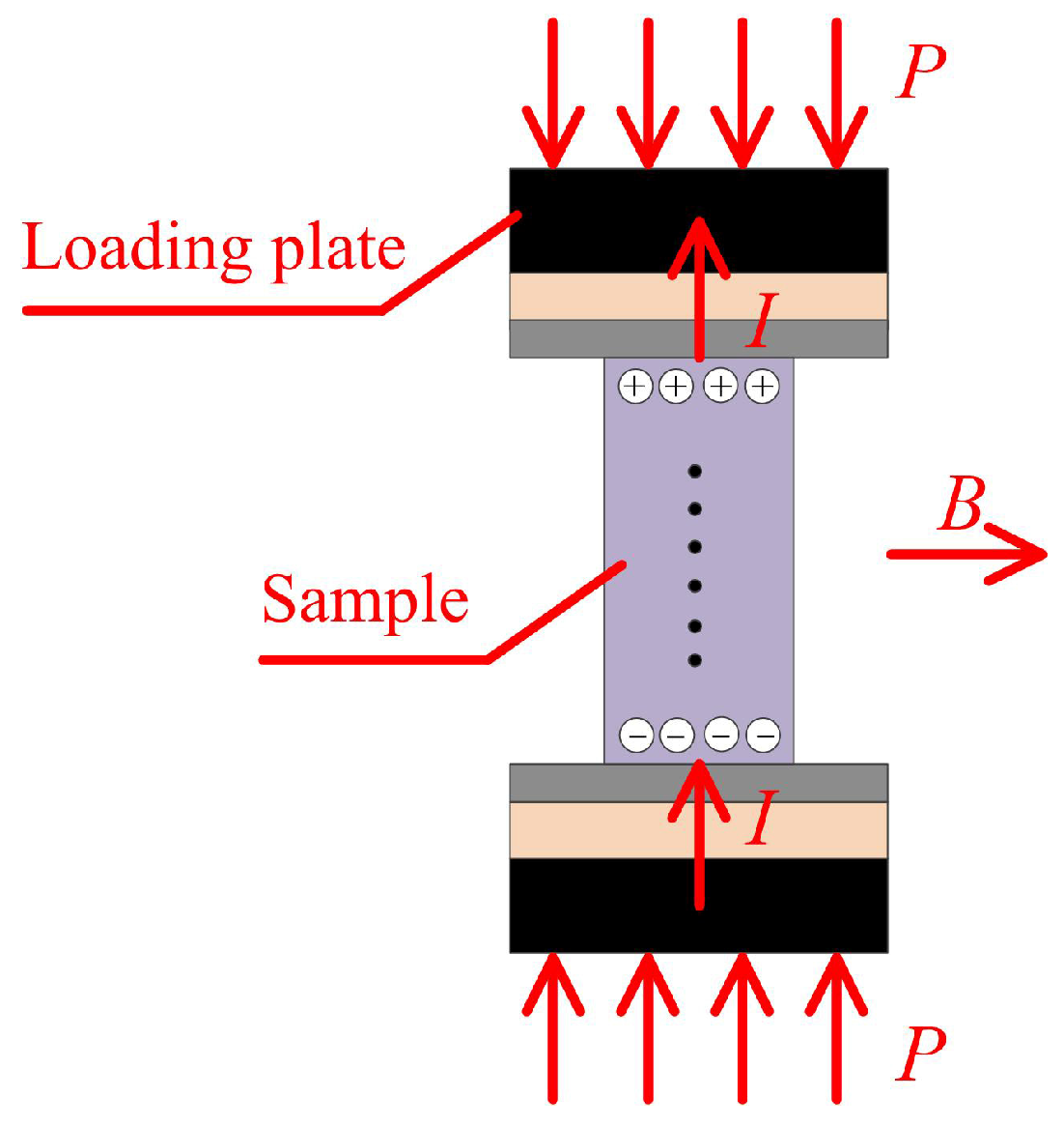
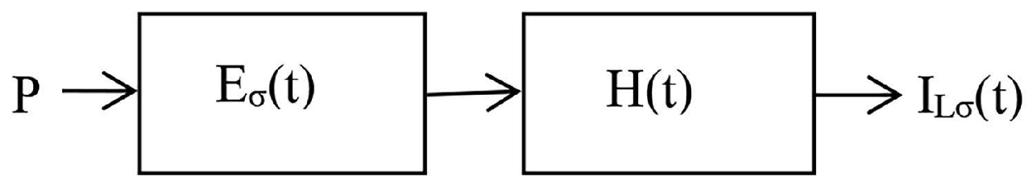
2.1. Electrophysical Analysis Model

Electromagnetic radiation will be produced in the process of compressive deformation and failure of rock. Figure 1 depicts a schematic diagram of a compression loading system with a rock specimen. The internal particles of the rock are not randomly distributed; rather, they are arranged in regular arrays, forming different structures. Both extrusion and shear deformation can change the structural configuration of the rock. Rock is cemented by mineral particles of different sizes, which are essentially composed of atoms. An atom consists of an atomic nucleus and electrons that orbit around it at high speed. In the absence of external forces, the rock appears uncharged and lacks electrical and magnetic properties. However, when an external compression load (P) is applied, the particles inside the rock are compressed or sheared, leading to a change in their structural configuration, known as particle structural configuration reset. During this process, the originally balanced electrons dissociate from the atomic nucleus and undergo polarization, as shown in Figure 2.
In Figure 2, the polarized electrons try to neutralize the positively charged cations in their free state. This physical phenomenon is the electric effect caused by the load on the specimen, which is called the piezoelectric effect. The schematic diagram of the current generation (I) is shown in Figure 2. Current (I) can be obtained by integrating the infinitesimal current density (i) on the cross-section of the specimen. It is expressed as:
I = i d S m
In Formula (1), Sm represents the microelement area of the cross-section in the specimen, measured in square meters (m2). The electromagnetic signal (B) emitted by the specimen is produced by current, measured in Teslas (T). The current, denoted as Iσ, is generated under the action of the load and is measured in amperes (A).
The electromotive force generated by the specimen, whether DC or AC, is expressed by Eσ, then
E σ = E d l
In Equation (2), E represents the electromotive force on a small length of the specimen under compression load, measured in volts (V). A potential difference, denoted as Uσ, exists at both ends of the specimen, as illustrated in the piezoelectric effect circuit model in Figure 3. The value of Uσ can be determined through measurement or calculation and is expressed in volts (V).
Since the loading device is a metal body, the electromotive force gathered at both ends of the specimen is equivalent to the short circuit of the conducting body, namely Uσ = 0 in Figure 4. During the loading process, displacement charge will continuously accumulate on the surfaces at both ends of the specimen. Under normal circumstances, the greater the pressure, the more displacement charge passes through the column of the loading device, and the greater the current flowing through the upper and lower plates, as shown in Figure 4 of the equivalent circuit model of the specimen under compression load. Assume that the current (Iσ) in Figure 4 flows from one end of the electromotive force (Eσ) and flows to the other end of the electromotive force (Eσ) through impedance (Zσ). The current (Iσ) will excite the magnetic field (B), that is, the electromagnetic signal radiated by the specimen. Therefore, in the field of electricity, this is clearly a problem of finding the system’s response at zero input. When there is no compression load (P), the input excitation (Eσ) of the circuit shown in Figure 4 is zero.

2.2. Materials and Processes

During the compression deformation process of rock samples, various types of electromagnetic radiation may be generated, including pulse electromagnetic radiation, low-frequency non-uniform amplitude oscillation electromagnetic radiation, and low-frequency uniform amplitude oscillation electromagnetic radiation. The purpose of this section’s experimental design was to analyze the changes in physical factors, such as voltage (Uσ), current (Iσ), impedance (Z), resistance (Rσ), capacitance (Z), and induced resistance (Z), caused by the compression deformation of rock samples. This analysis aimed to verify the electrical signal mode generated by the reset of particle structure.

2.2.1. Experimental Samples

Taking into account that the electrical physical parameters of different types of rocks may vary under the action of external loads, this experiment selected common sandstone, granite, and similar materials to make samples. Among them, two sources of granite material were chosen for the study: granite No. 8 from Fujian, China, and granite No. 9 from Henan, China (refer to Figure 5).
(1)
Rock samples
The sandstone and granite stone were processed into samples with dimensions of 70 mm × 70 mm × 70 mm. The end face of each sample was perpendicular to the axis with a deviation angle of less than 0.25°. The errors along the height and width of the sample were less than 0.3 mm. The surface roughness of the sample was 12.3 μm and the flatness was 0.1 mm.
(2)
Cement mortar sample
The rock-like samples were made using a mix of white cement, fine sand, and water in a mass ratio of 1:1.23:0.42. The fine sand used was sieved through a 1 mm mesh during the mixing process. The specimen had dimensions of 70 mm × 70 mm × 70 mm, with a surface roughness of 12.3 μm and a flatness tolerance of 0.1 mm.

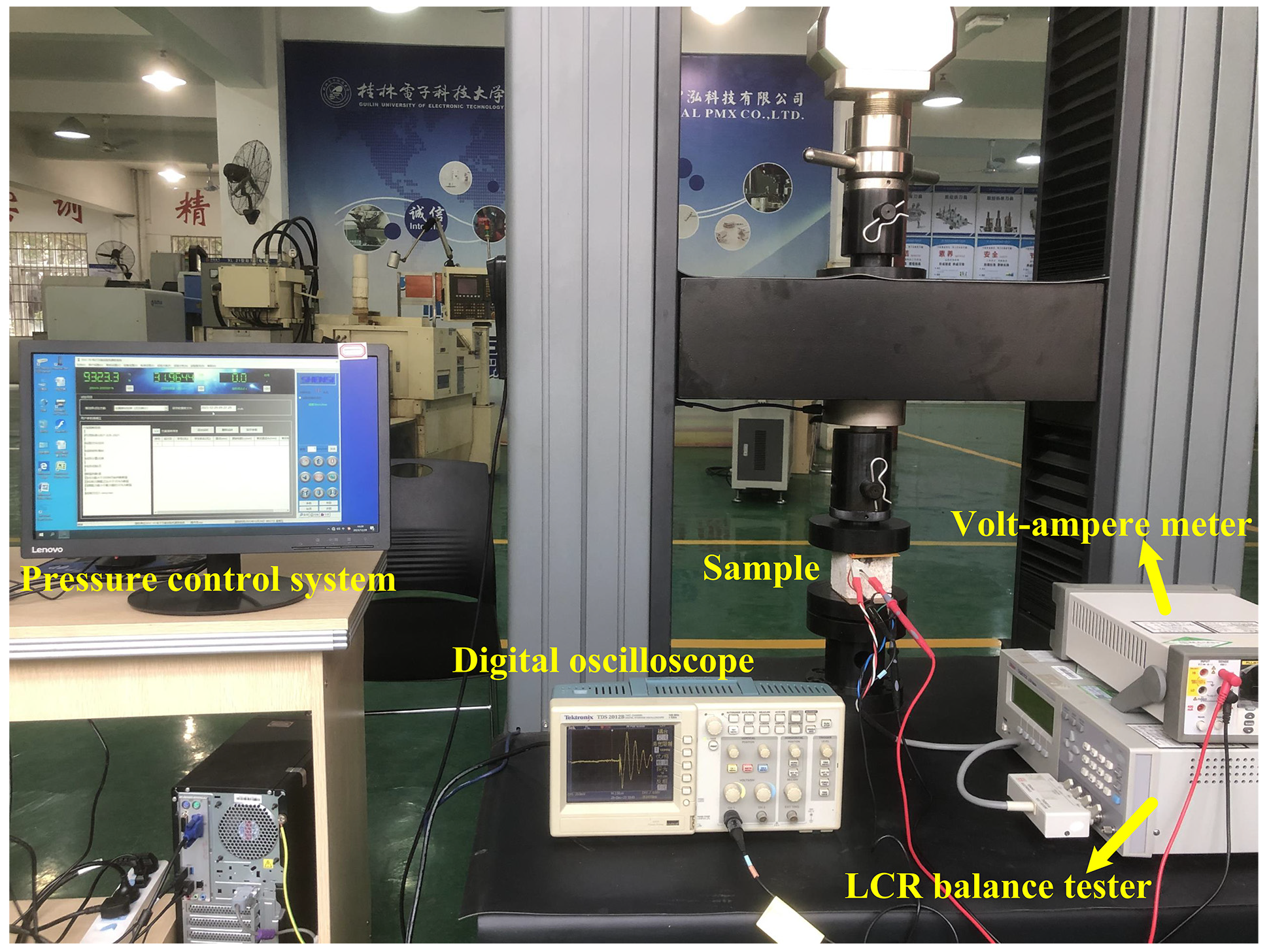
2.2.2. Experimental System

The measurement system, illustrated in Figure 6, consisted of a pressure testing machine, a digital oscilloscope, a 6.5-digit high-precision voltage and current meter (model: Fluke 8845a), an LCR balance tester, and a sample. The pressure testing machine had a load capacity of 30 tons, used to apply compressive load to the specimen. The digital oscilloscope observed the waveform of the voltage signal. The 6.5-digit high-precision voltage and current meter measured the open-circuit voltage and short-circuit current at the ends of the specimen. Lastly, the LCR balance tester measured the micro-element total resistance, capacitance, and inductance of the specimen under load.

2.2.3. Experiment Process

In Figure 6, the specimen was placed on the loading pad of the pressure testing machine and connected to the physical parameter measuring instruments. Then, the hydraulic testing machine was started, and various levels of compressive load were applied to the specimen. During this process, the open-circuit voltage (Uσ), short-circuit current (Iσ), microelement total resistance (Rσ), capacitance (Cσ), and inductance (Lσ) of the specimen were measured. The compressive loads applied were 2 kN, 4 kN, 6 kN, 8 kN, and 10 kN. The specific steps are outlined as follows:
(1) The specimen was placed on the loading pad and two electrodes were installed on its two end faces. The physical parameter measuring instruments were connected correctly.
(2) The initial physical parameters of the specimen, including total resistance, capacitance, inductance, voltage, and current, were recorded before applying the load (i.e., under zero load conditions).
(3) The experiment was conducted under normal temperature conditions at 20 °C, using a load-controlled method with a loading rate set to 100 N/s. Before the automatic loading program officially started, we manually initiated the loading device, adjusted the press head to approach the test specimen, and then stopped. Subsequently, the automatic loading program of the preset press was activated, and the load gradually increased from 0 to the predetermined load levels, at which point the automatic control system for load and displacement began recording the relevant data. The specific load levels were 2 kN, 4 kN, 6 kN, 8 kN, and 10 kN, with each test specimen undergoing this loading process five times. Each time the load reached the specified level, the corresponding electrical physical parameter values were recorded.
Furthermore, by applying different levels of load to the same specimen in this study, we were able to more accurately assess the mechanical behavior of the material under different stress levels. This method enhanced the comparability and reliability of the measurement results. It should be noted that when measuring the micro-element capacitance, inductance, and other physical parameters of the specimen under zero load conditions, the signal source reference frequency provided by the LCR impedance tester was set to 10 kHz. On the other hand, when measuring the open-circuit voltage and short-circuit current between the upper and lower electrodes of the pressure machine, the measuring instruments for voltage and current needed to be set to AC mode.

3. Results

In different load grade conditions, electrical parameter testing experiments were conducted on sandstone, granite, and similar rock material specimens, and the measured results of microelement total resistance, total inductance, total capacitance, voltage, current, and frequency are presented in Table 1.
Based on Table 1, the electrical signal pattern of the tested specimen showed periodic oscillation. The resistance (Rσ) and capacitance (Cσ) of the specimen were measured using an LCR impedance tester. When P = 0, the LCR impedance tester measured the inductance (Lσ) of the specimen as negative, indicating there was no inductance in the specimen. However, when P ≠ 0, the oscilloscope obtained a signal waveform showing attenuation oscillation. At this point, the dynamic total impedance (Zσ) of the specimen was obviously smaller than the resistance (Rσ). The total impedance (Zσ) was determined by using open-circuit voltage and short-circuit current. For instance, in the case of the 8# granite sample, when P = 2 kN, Zσ was measured to be 264.9 Ω (Zσ = Uσ/Iσ), whereas Rσ = 131,000.0 Ω. The inductance values in Table 1 were obtained using the formula 2πf = (LσCσ)−1/2. Further discussion will be needed to address the issue of the dynamic AC impedance Zσ being much smaller than the resistance Rσ.

4. Discussion

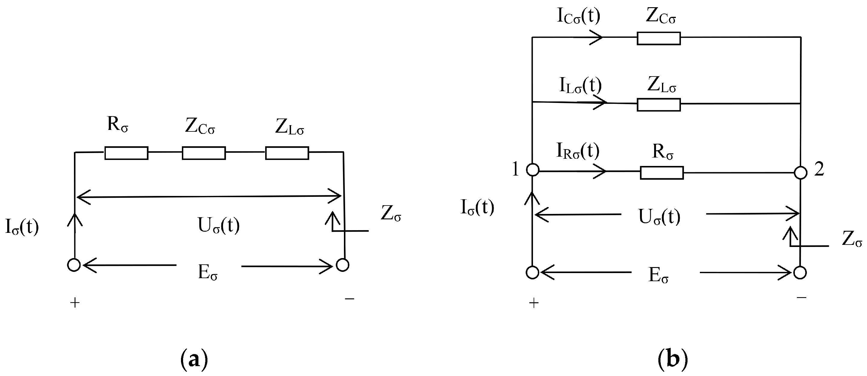
4.1. Passive Form of Signal Source and Circuit System Model

Considering the specimen as a system, the circuit shown in Figure 3 or Figure 4 is transformed into the circuit system (H(t)) shown in Figure 7, which is called a piezoelectric conversion system. In Figure 7, the compressive load (P) applied to the specimen is used as the excitation source of the circuit system (H(t)), which will cause the generation of an electric potential (Eσ(t)) within the specimen. The input excitation Eσ(t) of the circuit system (H(t)) is not generated by measurement instruments, so it is called a passive source. Analyzing the input excitation Eσ(t) and solving the output response of the circuit system (H(t)) is a very worthwhile issue. According to the experimental results, the existence of electric signals can be detected at very low load levels. This means that when a very low load is applied, the particle organization structure of the specimen is reset and electromagnetic radiation occurs. At a certain level of load, the typical waveform of the specimen is shown in Figure 8, which is the voltage waveform of 8# granite specimen under a load of 2 kN. This shows that the signal in the circuit system (H(t)) is attenuating and oscillating. Below is an analysis of this.
At t = 0, a compressive load (P) is applied, which leads to the excitation of the electric potential (Eσ(t)) and the beginning of charging the capacitance (Cσ). As time (t) increases and the compressive load (P) continues to act, the voltage (U(t)) across the capacitor’s terminals will also gradually increase. The voltage (U(t)) can be expressed as:
U C σ ( t ) = E σ ( t ) 1 e t / τ
In the formula, τ = RσCσ. When the load (P) rises to a predetermined value, U(t) increases to its maximum value, i.e., U(t) = Eσ(t). According to Formula (3), the charging curve exhibits an exponential monotonic increasing trend. Once the compressive load (P) is stopped, the capacitor begins to discharge, and the discharge pattern can be expressed as:
U C σ ( t ) = E σ ( t ) e t / τ
According to Expression (4), the discharge curve exhibits an exponential monotonic decay. Therefore, in the circuit system (H(t)), in addition to the energy-consuming element, resistance (Rσ), there are two different energy storage elements—inductance (Lσ) and capacitance (Cσ). Only when Lσ, Cσ, and Rσ all exist in the circuit system (H(t)) will the attenuation oscillatory discharge process occur. This shows that it is not comprehensive to study electromagnetic radiation by analyzing pure capacitor energy storage discharge (i.e., a single cause is the capacitor).

4.2. Identification of Circuit System Pattern

Figure 8 shows that the excitation and response of the circuit system (H(t)) is a dynamic attenuation second-order system composed of LCR elements. To determine whether the system is composed of series or parallel LCR elements, a circuit system model must be established and theoretical analysis must be conducted, as shown in Figure 9. Figure 9 includes second-order circuit systems (H(t)) composed of LCR elements in series or parallel. When the circuit is in its initial state (t = 0), the load P has Uσ(0) = Eσ at t = 0. The following mathematical model was established to solve for the impedance (Zσ), current (Iσ(t)), and voltage (U(t)). We assumed that “t = 0” denotes an instant just before t = 0.
(1)
The component of impedance and its mathematical model of output voltage response
When the specimen is not under external compressive loading, it is assumed that the initial impedance is Z0; the initial impedance (Z0) is composed of the microelement total resistance (R0) and the capacitive reactance (Z). However, when the specimen is subjected to external loading, its microstructural configuration changes with stress, and the impedance value of the specimen is no longer Z0, but a dynamic quantity composed of the microelement total resistance (R0), the capacitive reactance (Z), and the inductive reactance (Z), etc. The microelement total resistance (R0), the capacitive reactance (Z), and the inductive reactance (Z) are the components of the total impedance (Zσ).
The theoretical expression for the impedance (Z) in the frequency domain is:
Z C σ = 1 / ( j ω C σ )
In Equation (5), j represents the reactance, which is in the form of a complex number; ω represents the angular frequency of the measurement instrument’s signal source; and Cσ is the total capacitance of the specimen. When this component is subjected to the excitation shown in Figure 9, its voltage response model is as follows.
U C σ ( t ) = 1 C 0 t I C σ ( t ) d t
The theoretical calculation expression of inductive impedance (Z) in the frequency domain is:
Z L σ = ( j ω L σ )
In Equation (7), Lσ is the dynamic inductance, which is expressed as
L σ = μ μ 0 S N 2 / l
In Equation (8), μ′ represents the magnetic permeability, μ0 represents the permeability of the vacuum, S represents the cross-sectional area of the specimen, l represents the length of the specimen, and N represents the number of turns in the coil. Since the specimen does not have a coil structure, the inductance (Lσ) is zero when the load is zero; while when the load is applied, the inductance (Lσ) is solved jointly by the total impedance (Zσ) and the capacitive impedance (Z).
In the system shown in Figure 9, the voltage response model of the inductive reactance (Z) under the excitation of Uσ(t) is as follows:
U L σ ( t ) = L d I L σ ( t ) / d t
The last physical quantity that affects the total impedance (Zσ) is the microelement total resistance (Rσ), and the formula for Rσ is:
R σ = ρ l / S
In Equation (10), ρ′ represents the electrical conductivity, l represents the length of the specimen, and S represents the cross-sectional area of the specimen. The electrical conductivity of the rock specimen, ρ′, is difficult to determine accurately, so the specific numerical value of Rσ is usually obtained through actual measurement. Under the excitation of Uσ(t), the model of the response voltage (Uσ(t)) of Rσ in the system shown in Figure 9 is as follows.
U R σ ( t ) = R σ I σ ( t )
(2)
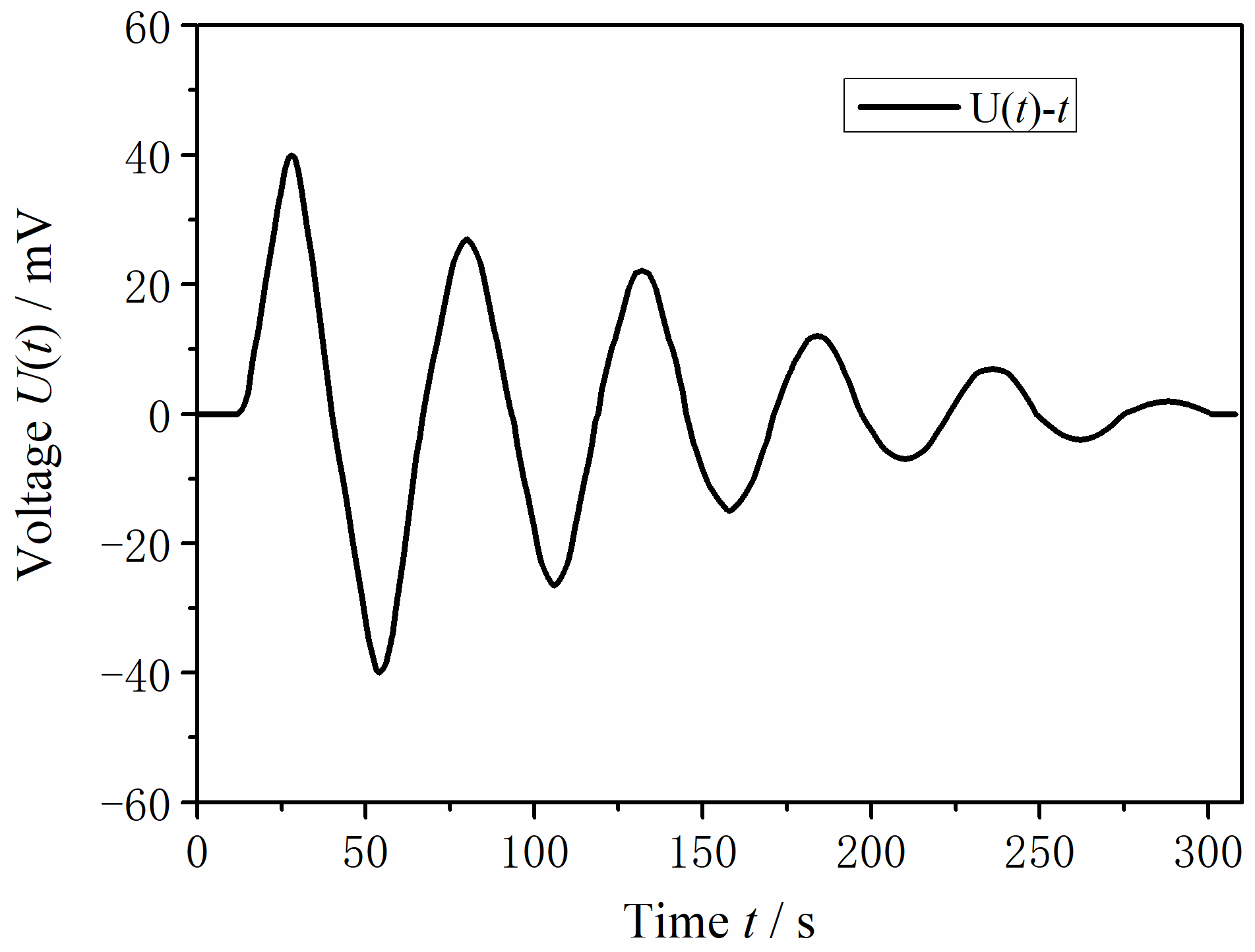
Identification of LCR series attenuating oscillation circuit
(1) Mathematical model of LC series second-order circuit system
The LCR components, representing the inductive impedance (Z), capacitive impedance (Z), and resistance (Rσ), are considered to be linked in series, as shown in Figure 9a. Based on Kirchhoff’s voltage law, the complex frequency domain mathematical model of the second-order system H(t) comprised of LCR components in series is given by:
U σ ( t ) = I σ ( t ) [ R σ + j ω L σ + 1 / ( j ω C σ ) ]
Converting Equation (12) to an equivalent model in the S-domain and simplifying it to obtain a mathematical model of the current in the S-domain, denoted as Iσ(S), then
I σ ( S ) = E σ / L σ S 2 + S R σ + 1 / ( L σ C σ )
Solve Equation (13) and obtain its characteristic roots as
P 1 = L σ 2 R σ + L σ 2 R σ 2 1 L σ C σ
P 2 = L σ 2 R σ L σ 2 R σ 2 1 L σ C σ
According to the above expression, after inverse transformation, the current equation flowing through the impedance (Zσ) is obtained, which is
I σ ( t ) = E σ L σ 1 P 1 P 2 e P 1 t e P 2 t
To determine whether the circuit in Figure 8 is a damped oscillation system, assuming α = L σ 2 R σ and ω 0 = 1 L σ C σ , then
P 1 = α + α 2 ω 0 2
P 2 = α α 2 ω 0 2
(2) The attenuation and oscillation conditions of LC series circuit and its determination
P1 and P2 are a pair of conjugated complex roots. When α < ω0 or Rσ < 2(LσCσ)1/2 (i.e., Rσ is small), the high-quality factor (Q) LσCσ circuit will satisfy Q = ω0/(2π), in which case, the circuit will undergo attenuated oscillation. The experimental results of the 8# granite specimen were used to verify the electrical decay oscillation system shown in Figure 8. When P = 2 kN, Rσ = 131 kΩ, f = 18.99 kHz, ω0 = 119.3 × 10³ rad/s, and when Cσ = 474 pF, Lσ = 148.2 mH, so α = Rσ/(2Lσ) = 441.97 × 10³. It can be seen that α > ω0, which contradicts the condition that α < ω0, so the circuit system (H(t)) cannot oscillate. That is, the circuit system (H(t)) is not the damped oscillation system presented in Figure 8, and the assumption of the LCR series attenuation oscillation circuit model is not valid.
(3)
Identification of LCR parallel attenuation oscillation circuit
(1) Mathematical model of LC parallel second-order circuit system
The components corresponding to inductive reactance (Z), capacitive reactance (Z), and resistance (Rσ) are denoted as LCR. The connection between LCR elements is in parallel, as shown in Figure 9b. To analyze the attenuation oscillation phenomenon (as shown in Figure 8) that occurs in the LCR parallel circuit system, an electromagnetic radiation-generating inductor response model I(t) at zero input state in the system needs to be established.
In accordance with Kirchhoff’s current law, the current entering node “1” in Figure 9b is equivalent to the current exiting the node, and can be described by the following relationship.
I σ ( t ) = I R σ ( t ) + I C σ ( t ) + I L σ ( t )
According to Equation (19), derive the characteristic equation of the second-order system, which is the impedance admittance.
U σ ( t ) Z σ = U R σ ( t ) R σ + U C σ ( t ) Z C σ + U L σ ( t ) Z L σ
Let 1/Zσ = Y, 1/Rσ = G, 1/Z = jωCσ, 1/Z = (jωLσ), substitute these values into Equation (20), and then simplify it according to the parallel circuit conditions.
Y = G + j ω C σ + 1 / ( j ω L σ )
Convert Equation (21) to an equivalent model in the S domain. Then, the characteristic equation of the zero-input response in the S domain is:
L σ C S 2 + G L σ S + 1 = 0
Solving Equation (22) yields the characteristic roots:
P 1 = 1 2 R σ C σ + 1 ( 2 R σ C σ ) 2 1 L σ C σ
P 2 = 1 2 R σ C σ 1 ( 2 R σ C σ ) 2 1 L σ C σ
If the damping coefficient of the circuit is α = 1/(2RσCσ) and the resonant frequency is ω20 = 1/(LσCσ), then
P 1 = α + α 2 ω 0 2
P 2 = α α 2 ω 0 2
According to the characteristic roots (P1, P2) of Equation (22), the solving equation for I(t) can be obtained through inverse transformation:
I L σ ( t ) = A 1 e P 1 t + A 2 e P 2 t
After undergoing time-domain and frequency-domain transformations, the current solution flowing through the impedance (Z) is obtained.
I L σ ( t ) = ( A 1 cos ω 0 t + A 2 sin ω 0 t ) e α t
In Equation (28), A1 and A2, respectively, represent the amplitudes of the currents, where A 1 = U C σ ( 0 ) L ( P 1 P 2 ) and A 2 = U C σ ( 0 ) L ( P 1 P 2 ) .
For specific rock materials that have not yet been deeply studied, the electromagnetic signals generated under compression are primarily manifested as direct current signals, signals with periodic variations, and signals with non-periodic variations. Regarding the Formula (28) that we have proposed, even when the rock material only generates a direct current signal, i.e., the frequency is zero, the sine term in the formula calculates to zero, yet the entire theoretical formula remains applicable. When the rock material generates a pulse signal under compression, we can decompose this signal into the fundamental wave and higher harmonics, and then substitute them into the theoretical formula for analysis, at which point the theoretical formula is still applicable. Furthermore, the theoretical analysis framework constructed in this study takes the example of a damped sinusoidal signal, and the derived theoretical formula naturally applies to such signals. Therefore, theoretically speaking, the results of our research can be extended to other types of geological materials. This indicates that our theoretical model has a wide applicability and can provide analysis and interpretation for the electromagnetic signals generated by different types of rock materials under compression.
At present, most studies tend to explore rock mechanics problems using individual physical quantities such as resistivity, dielectric constant (permittivity), and magnetic permeability. In contrast, our constructed model (see Equation (28) for details) integrates these physical quantities into a comprehensive analytical framework. From the perspective of integrating multiple physical factors to construct a theoretical analysis model, our model provides a unified method of physical analysis. Looking from the angle of signal types, the model we have established is capable of fully adapting to the analysis needs of different types of signals, whether these are direct current signals, signals with periodic change patterns, or signals with non-periodic change patterns, all are applicable. This indicates that the model we have constructed is a comprehensive tool for physical analysis. For specific rock materials that have not been deeply studied, the electromagnetic signals they generate under compression are also no more than manifestations of these types of physical signals. Therefore, we believe that this model is a truly unified physical analysis model, which can provide a solid theoretical foundation for in-depth research in rock mechanics.
(2) The attenuation and oscillation conditions of LC parallel circuit and its determination
To further analyze the oscillation transition process of the circuit system shown in Figure 9b in the underdamped state, the particular solution of I(t) was obtained. According to P1 = −α + (α2ω20)1/2 and P2 = −α − (α2ω20)1/2, its characteristic root is a pair of complex conjugate roots. When the condition α < ω0, (2RσCσ)−2 − (RσCσ)−1 < 0, or Rσ > 1/2(RσCσ)−1/2 < 0 is met, the circuit system in Figure 9b will exhibit oscillations in an underdamped state. Next, the experimental results of the 8# granite specimen were used to analyze whether the circuit in Figure 9b meets the damped oscillation condition. When P = 2 kN, Rσ = 131 kΩ, f = 18.99 kHz, then ω0 = 2πf = 119.3 × 10³ rad/s, and when Cσ = 474 pF, Lσ = 148.2 mH, then α = 1/(2LσRσ) = 8052 ΩF−1. It can be seen that the experimental results meet the condition of α < ω0, so the circuit system in Figure 9b can oscillate. That is to say, the circuit system in Figure 9b meets the damped oscillation transition requirements presented in Figure 8, and the assumption of the parallel circuit model is valid.

4.3. Variation of Impedance during Loading

Without any load applied, the total impedance (Zσ) equals the initial value (Z0). The initial value of Zσ may vary depending on the rock type, as indicated in Table 2. When a load is applied to the specimen and the electrodes at both ends are open circuit, the voltage Uσ(t) at both ends of the specimen is equal to the potential (Eσ(t)). If the relationship between Uσ(t), Iσ(t), and Zσ follows Ohm’s law of complex impedance, then
U σ ( t ) / Z σ = I σ ( t )
In Equation (29), Zσ represents the total microelement impedance of the specimen. The value of the total microelement impedance (Zσ) is closely related to the total resistance (Rσ), total capacitance (Z), and total inductance (Z) of the specimen. The total microelement impedance (Zσ) of the specimen directly measured using an LCR instrument is listed in Table 2. According to Table 2, as the load (P) increases, the total microelement impedance (Zσ) of the specimen shows a decreasing trend.
Table 2. Test results for dynamic impedance and resistance of various rock specimens under load.
Load
P (kN)
0246810
 8# Granite sample
Zσ(t) (kΏ)00.2640.1020.3260.3090.480
Zσ(0) (kΏ)374.0146.0129.0119.0112.0106.0
Rσ (kΏ)171.0131.0120.0113.0107.0102.0
 9# Granite sample
Zσ(t) (kΏ)00.6971.5971.4061.4971.296
Zσ(0) (kΏ)965.0887.0890.0862.0853.0841.0
Rσ (kΏ)730.0681.0652.0641.0637.0633.0
 11# Red sandstone sample
Zσ(t) (kΏ)01.8092.0241.4572.0311.943
Zσ(0) (kΏ)861.0114.069.056.047.044.0
Rσ (kΏ)56.045.032.029.027.025.0
 10# Cement mortar sample
Zσ(t) (kΏ)02.2335.1383.6792.0502.739
Zσ(0) (kΏ)3285.02790.02720.02660.02620.02580.0
Rσ (kΏ)3940.03020.02890.02810.02750.02690.0
The aforementioned types of rocks exhibit different dynamic impedance values when subjected to the same level of load (see Table 2). This indicates that the dynamic impedance characteristics of rocks are correlated with their types. Generally speaking, granite is primarily composed of quartz, feldspar, and mica, with a typically high content of quartz. Sandstone, on the other hand, is mainly composed of sand particles (usually quartz, feldspar fragments, or rock debris), with a sand content usually exceeding 50%. However, the quartz content in sandstone is not as significant as in granite. Research by Wei et al. [28] has shown that the quartz content does not stimulate the activity and intensity of the electromagnetic radiation (EMR) signals generated by rock fracture. Secondly, changes in dynamic impedance involve resistance, capacitance, and inductance. Generally, due to its higher porosity, sandstone typically exhibits higher capacitance values, which, in turn, results in higher dynamic impedance values [35,36]. This can be reflected in the capacitance measurements from Table 1 and the dynamic impedance measurements from Table 2. Regarding the orientation of minerals, minerals in granite have a certain degree of orientation, but this orientation is usually weak; the sand particles and cementing materials in sandstone may exhibit a stronger orientation, especially in the layered structures formed during the sedimentation process. When subjected to the same level of load, the mineral orientation in sandstone is more disturbed, leading to a more intense reset of the internal particle organization configuration, thereby exhibiting a greater dynamic impedance value. Although there are significant differences between different rock types, this study found that the dynamic impedance of different rock types shows a consistent overall downward trend, which can be generalized to a broader range of rock materials. However, to specifically reveal the correlation between the dynamic impedance characteristics of rocks and specific rock types and their microstructural properties, further research using techniques such as scanning electron microscopy (SEM) and X-ray micro-computed tomography (X-CT) will be required in the future.

4.4. The Variation of Voltage and Current Generated by the Specimen under the Action of Load

During the deformation and damage process of the specimen under load, in addition to direct-current pulsed electromagnetic radiation, there will also be low-frequency non-uniform attenuation oscillation. Below is an analysis of the variation patterns between open-circuit voltage (Uσ(t)), short circuit current (Iσ(t)), and load (P). Figure 10 illustrates the curve of the open-circuit voltage (Uσ(t)) with respect to load (P), where this voltage represents the electromotive force generated by the specimen under loading conditions. It should be noted that the prerequisite for measuring the open-circuit voltage is to isolate the sample’s two ends and the loading pad of the pressure machine through insulating boards. From this figure, it can be seen that electromotive force generally increases with higher loads but exhibits significant fluctuations.
The curve of the short-circuit current (Iσ(t)) versus the load (P) is shown in Figure 11. Here, the short-circuit current refers to the current that forms a natural loop circuit between the test piece and the pressure machine when the upper and lower plates of the pressure machine are not separated from the test piece by an insulating plate under the load. The overall trend of the current increases as the load increases, but it fluctuates greatly.
Based on the experimental results, it is clear that both cement mortar specimens and other rock specimens exhibit a reset in particle structure when subjected to small loads, leading to the generation of piezoelectric effects. This means that electromagnetic radiation is consistently produced as the specimen undergoes loading. Moreover, the current intensity generated by specimens of different rock types under various load excitations varies, resulting in differences in electromagnetic radiation intensity. The phenomenon of the current intensity not always increasing for the same specimen under different load excitations is associated with the reset state of the specimen’s internal microstructure configuration.
Furthermore, the voltage amplitude and current intensity are not always directly correlated. For instance, the 10# cement mortar specimen, when P = 4 kN, has a voltage amplitude of up to 400.8 mV, but only a current of 78 µA; when P = 4 kN, the voltage amplitude of the 8# granite specimen is only 9 mV, but it has a higher current of 88 µA. This discrepancy is associated with the rock type and internal microstructure configuration of the sample. It can be seen that it is feasible to analyze and continuously track the compressive deformation and damage of different rock samples by using the parallel circuit model consisting of dynamic physical quantities Uσ, Iσ, Cσ, Lσ, and Rσ.
Additionally, this study has selected common granite and sandstone as the subjects of research. However, the complexity of structural characteristics in the study subjects, such as samples with heterogeneous rock structures, and the discrepancies between the sample sizes in experimental conditions and actual engineering practices, have limited the applicability of the experimental results in assessing the electromagnetic radiation patterns of larger-sized samples under compression. In actual engineering applications, the methods of applying compressive loads are diverse and do not completely align with experimental conditions. Furthermore, since the loads applied in the experiments did not cause the samples to fail, there are limitations in the simulation of real-world load responses by the experimental load conditions. In practical engineering applications, the samples often involve larger sizes, and the amplitude of the radiation signal strength produced by these samples under compression presents a technical challenge that needs to be addressed.
Beyond the challenges faced in the practical application domain, this study actually holds significant practical importance. Theoretically, the established electrophysical model is capable of intuitively and accurately depicting the variations in electromagnetic signals of rocks under different compressive loads. The circuit analysis model, which incorporates inductance, capacitance, and resistance, further facilitates the transformation of electromagnetic signal detection into the detection of voltage or current, offering considerable convenience. Based on these physical parameters, subsequent work can apply the theory of damage mechanics to formulate a mathematical model that characterizes damage using the parameter of electromagnetic signals generated by the reconfiguration of particle organization in compressed rocks. This model has important applications in rock mechanics.
On the foundation of understanding the relationship between compressive load and electromagnetic signals, and with the aid of a substantial amount of actual experimental data, including data influenced by size effects, it is possible to acquire precursor information about the deformation and failure of rocks under compressive loads, thereby more accurately monitoring and predicting the deformation and failure processes of rocks. This is of great significance for the early identification of potential rock disasters, such as the instability of tunnel-surrounding rocks during excavation.
To realize the translation of its practical application, detection sensors can be developed based on the established electrophysical model to capture information on the electromagnetic signals of rocks. The objective is to establish an early warning system in the fields of rock mechanics, geophysics, and dynamic rock disaster early warning systems, which will predict potential rock disasters by monitoring the electromagnetic signals of rocks in real time.

5. Conclusions

In order to investigate the dynamic electrical signals generated by rocks, compression tests were conducted on samples of four different rock types under varying load levels. The resulting changes in dynamic physical parameters, including voltage, current, frequency, and impedance, due to particle structure reorganization under load were studied. Additionally, an electrical model for analyzing particle organization structure reorganization was developed and a theoretical analysis of the circuit system governing signal changes was conducted based on experimental results. The following conclusions were drawn:
(1) By transforming the deformation and damage analysis of the specimen under compressive load into an analysis of the circuit’s physical parameters, an electrical physical model was established for the reorganization of the particle organization structure of rock specimens under compressive load.
(2) Under compressive loading, the internal structure of the rock specimen undergoes reorganization, resulting in the generation of damped oscillating currents that act as a source of electromagnetic radiation signals. Throughout the loading process, there is a continuous current flow closely associated with both the loading and the reorganized state of the specimen’s internal structure. With increasing external compressive loading, there is an overall trend of increased current strength and correspondingly enhanced amplitude of electromagnetic radiation signals generated within the specimen.
(3) During the loading process, the physical parameters of the specimen, such as Rσ, the body resistance; Cσ, the body capacitance; and Lσ, the body inductance, are dynamically changing. When the external compressive load increases, the impedance (Z) corresponding to the body resistance (Rσ) and the body capacitance (Cσ) decrease, while the trend of the impedance (Z) corresponding to the body inductance (La) is not obvious. The changes of Rσ, Cσ, and Lσ dominate the current (Iσ(t)) and are related to the reorganization of particle structures within the specimen.
(4) A circuit system model was established for analyzing the parallel resistances (Rσ), capacitances (Cσ), and inductances (Lσ) of different rock materials, including granite, sandstone, and cement mortar. The analysis results obtained from the model were in agreement with the actual findings from experimental tests.
When a rock specimen is subjected to compressive deformation, the internal resistance (Rσ), capacitance (Cσ), and inductance (Lσ) of the specimen will inevitably change, causing fluctuations in energy dissipation. The next step of the study is to develop a mathematical model that represents rock damage using dynamic physical parameters based on the electrical physical model of the rock specimen deformation. This analysis aims to deeply understand the changes in electromagnetic energy dissipation during rock damage.

Author Contributions

Conceptualization, C.O. and B.M.; methodology, C.O. and B.M.; validation, C.O., X.Z. and H.C.; formal analysis, X.Z. and H.C.; investigation, X.Z., B.M. and H.C.; resources, C.O. and H.C. All authors have read and agreed to the published version of the manuscript.

Funding

This research was supported by the Specific Research Project of Guangxi for Research Bases and Talents (Grant No. AD23026103) and the Middle-Aged and Young Teachers’ Basic Ability Promotion Project of Guangxi (Grant No. 2023KY0203).

Institutional Review Board Statement

Not applicable.

Informed Consent Statement

Not applicable.

Data Availability Statement

The raw data supporting the conclusions of this article will be made available by the corresponding author on request.

Conflicts of Interest

The authors declare that they have no known competing financial interests or personal relationships that could appear to have influenced the work reported in this paper.

References

  1. Wang, Z.; Wang, M.; Zhou, L.; Zhu, Z.; Shu, Y.; Peng, T. Research on uniaxial compression strength and failure properties of stratified rock mass. Theor. Appl. Fract. Mech. 2022, 121, 103499. [Google Scholar] [CrossRef]
  2. Du, S.; Ma, J.; Ma, L.; Zhao, Y. Unconfined compressive strength and failure behaviour of completely weathered granite from a fault zone. J. Mt. Sci.-Engl. 2024, 21, 2140–2158. [Google Scholar] [CrossRef]
  3. Frid, V.; Goldbaum, J.; Rabinovitch, A.; Bahat, D. Electric polarization induced by mechanical loading of Solnhofen limestone. Phil. Mag. Lett. 2009, 89, 453–463. [Google Scholar] [CrossRef]
  4. Kaselow, A.; Shapiro, S.A. Stress sensitivity of elastic moduli and electrical resistivity in porous rocks. J. Geophys. Eng. 2004, 1, 1. [Google Scholar] [CrossRef]
  5. Jia, P.; Wang, Q.; Qian, Y.; Wang, Y. Variation characteristics of electric resistance in the quiet periods of acoustic emission of sandstone with different saturation. J. Cent. South Univ. 2023, 30, 1993–2003. [Google Scholar] [CrossRef]
  6. Wang, K.; Xia, Z.; Huang, Z.; Li, X. Damage Evolution of Sandstone under Constant-Amplitude Cyclic Loading Based on Acoustic Emission Parameters and Resistivity. Adv. Mater. Sci. Eng. 2021, 2021, 7057183. [Google Scholar] [CrossRef]
  7. Li, X.; Zhang, Q.; An, Z.; Chen, X.; Zhang, F. Experimental research on electrical resistivity variation of coal under different loading modes. Arab. J. Geosci. 2020, 13, 1068. [Google Scholar] [CrossRef]
  8. Qu, C.; Xue, Y.; Su, M.; Qiu, D.; Ma, X.; Liu, Q.; Li, G. Quantitative modeling of rock electrical resistivity under uniaxial loading and unloading. Acta Geophys. 2024, 72, 195–212. [Google Scholar] [CrossRef]
  9. Li, M.; Wang, H.; Wang, D.; Shao, Z. Experimental study on characteristics of surface potential and current induced by stress on coal mine sandstone roof. Eng. Geol. 2020, 266, 105468. [Google Scholar] [CrossRef]
  10. Li, W.; Fang, S.; Gao, X. Experimental investigation on the influence of wave impedance on dynamic mechanical response of granites undergone high temperature. ACS Omega 2023, 8, 42398–42408. [Google Scholar] [CrossRef] [PubMed]
  11. Negi, P.; Chakraborty, T.; Bhalla, S. Viability of electro-mechanical impedance technique for monitoring damage in rocks under cyclic loading. Acta Geotech. 2022, 17, 483–495. [Google Scholar] [CrossRef]
  12. Li, M.; Lu, Y.; Shi, S.; Wang, D.; He, S.; Ye, Q.; Li, H.; Zhu, S.; Wang, Z. The variation of micro-current in rock under loads and its microcosmic influence mechanism. Eng. Geol. 2022, 310, 106877. [Google Scholar] [CrossRef]
  13. Brady, B.T.; Rowell, G.A. Laboratory investigation of the electrodynamics of rock fracture. Nature 1986, 321, 488–492. [Google Scholar] [CrossRef]
  14. Cress, G.O.; Brady, B.T.; Rowell, G.A. Sources of electromagnetic radiation from fracture of rock samples in the laboratory. Geophys. Res. Lett. 1987, 14, 331–334. [Google Scholar] [CrossRef]
  15. Fukui, K.; Okubo, S.; Terashima, T. Electromagnetic radiation from rock during uniaxial compression testing: The effects of rock characteristics and test conditions. Rock Mech. Rock Eng. 2005, 38, 411–423. [Google Scholar] [CrossRef]
  16. Hadjicontis, V.; Mavromatou, C. Transient electric signals prior to rock failure under uniaxial compression. Geophys. Res. Lett. 1994, 21, 1687–1690. [Google Scholar] [CrossRef]
  17. Yoshida, S.; Uyeshima, M.; Nakatani, M. Electric potential changes associated with slip failure of granite: Preseismic and coseismic signals. J. Geophys. Res.-Solid Earth 1997, 102, 14883–14897. [Google Scholar] [CrossRef]
  18. Rabinovitch, A.; Frid, V.; Bahat, D.; Goldbaum, J. Fracture area calculation from electromagnetic radiation and its use in chalk failure analysis. Int. J. Rock Mech. Min. 2000, 37, 1149–1154. [Google Scholar] [CrossRef]
  19. Carpinteri, A.; Lacidogna, G.; Manuello, A.; Niccolini, G.; Schiavi, A.; Agosto, A. Mechanical and electromagnetic emissions related to stress-induced cracks. Exp. Tech. 2012, 36, 53–64. [Google Scholar] [CrossRef]
  20. Yamada, I.; Masuda, K.; Mizutani, H. Electromagnetic and acoustic emission associated with rock fracture. Phys. Earth Planet. Inter. 1989, 57, 157–168. [Google Scholar] [CrossRef]
  21. Frid, V.; Rabinovitch, A.; Bahat, D. Fracture induced electromagnetic radiation. J. Phys. D Appl. Phys. 2003, 36, 1620–1628. [Google Scholar] [CrossRef]
  22. Frid, V.; Vozoff, K. Electromagnetic radiation induced by mining rock failure. Int. J. Coal Geol. 2005, 64, 57–65. [Google Scholar] [CrossRef]
  23. Qiu, L.; Liu, Z.; Wang, E.; He, X.; Feng, J.; Li, B. Early-warning of rock burst in coal mine by low-frequency electromagnetic radiation. Eng. Geol. 2020, 279, 105755. [Google Scholar] [CrossRef]
  24. Ogawa, T.; Oike, K.; Miura, T. Electromagnetic radiations from rocks. J. Geophys. Res. Atmos. 1985, 90, 6245–6249. [Google Scholar] [CrossRef]
  25. Song, M.; Hu, Q.; Liu, H.; Li, Q.; Zhang, Y.; Hu, Z.; Liu, J.; Deng, Y.; Zheng, X.; Wang, M. Characterization and correlation of rock fracture-induced electrical resistance and acoustic emission. Rock Mech. Rock Eng. 2023, 56, 6437–6457. [Google Scholar] [CrossRef]
  26. Baddari, K.; Frolov, A.D.; Tourtchine, V.; Rahmoune, F. An integrated study of the dynamics of electromagnetic and acoustic regimes during failure of complex macrosystems using rock blocks. Rock Mech. Rock Eng. 2011, 44, 269–280. [Google Scholar] [CrossRef]
  27. Han, J.; Huang, S.; Zhao, W.; Wang, S.; Deng, Y. Study on electromagnetic radiation in crack propagation produced by fracture of rocks. Measurement 2019, 131, 125–131. [Google Scholar] [CrossRef]
  28. Wei, M.; Song, D.; He, X.; Li, Z.; Qiu, L.; Lou, Q. Effect of rock properties on electromagnetic radiation characteristics generated by rock fracture during uniaxial compression. Rock Mech. Rock Eng. 2020, 53, 5223–5238. [Google Scholar] [CrossRef]
  29. Li, X.; Li, H.; Yang, Z.; Li, Y.; Li, H.; Zhou, J. The influence of the internal structure of loaded composite coal-rock on the variation characteristics of electromagnetic radiation (EMR) signal. J. Appl. Geophys. 2023, 213, 105027. [Google Scholar] [CrossRef]
  30. Xiao, H.; He, X.; Wang, E. Research on transition law between EME and energy during deformation and fracture of coal or rock under compression. Rock Soil Mech. 2006, 27, 1097–1100. (In Chinese) [Google Scholar] [CrossRef]
  31. Nie, B.; He, X.; Wang, E.; Li, G.; Liu, W. Coupled stress-electricity model and its parameters computation method of coal or rock. J. China Univ. Min. Technol. 2007, 36, 505–508. (In Chinese) [Google Scholar]
  32. Li, Z.; Zhang, X.; Wei, Y.; Ali, M. Experimental study of electric potential response characteristics of different lithological samples subject to uniaxial loading. Rock Mech. Rock Eng. 2021, 54, 397–408. [Google Scholar] [CrossRef]
  33. Triantis, D.; Pasiou, E.D.; Stavrakas, I.; Kourkoulis, S.K. Hidden affinities between electric and acoustic activities in brittle materials at near-fracture load levels. Rock Mech. Rock Eng. 2022, 55, 1325–1342. [Google Scholar] [CrossRef]
  34. Wan, G.; Li, X.; Hong, L. Piezoelectric responses of brittle rock mass containing quartz to static stress and exploding stress wave respectively. J. Cent. South Univ. 2008, 15, 344–349. [Google Scholar] [CrossRef]
  35. Hafez, A.; Castagna, J.P. Distinguishing gas-bearing sandstone reservoirs within mixed siliciclastic-carbonate sequences using extended elastic impedance: Nile Delta—Egypt. Interpret.-J. Subsurf. Charact. 2016, 4, T427–T441. [Google Scholar] [CrossRef]
  36. Kirichek, A.; Chassagne, C.; Ghose, R. Predicting the dielectric response of saturated sandstones using a 2-electrode measuring system. Front. Phys. 2019, 6, 148. [Google Scholar] [CrossRef]
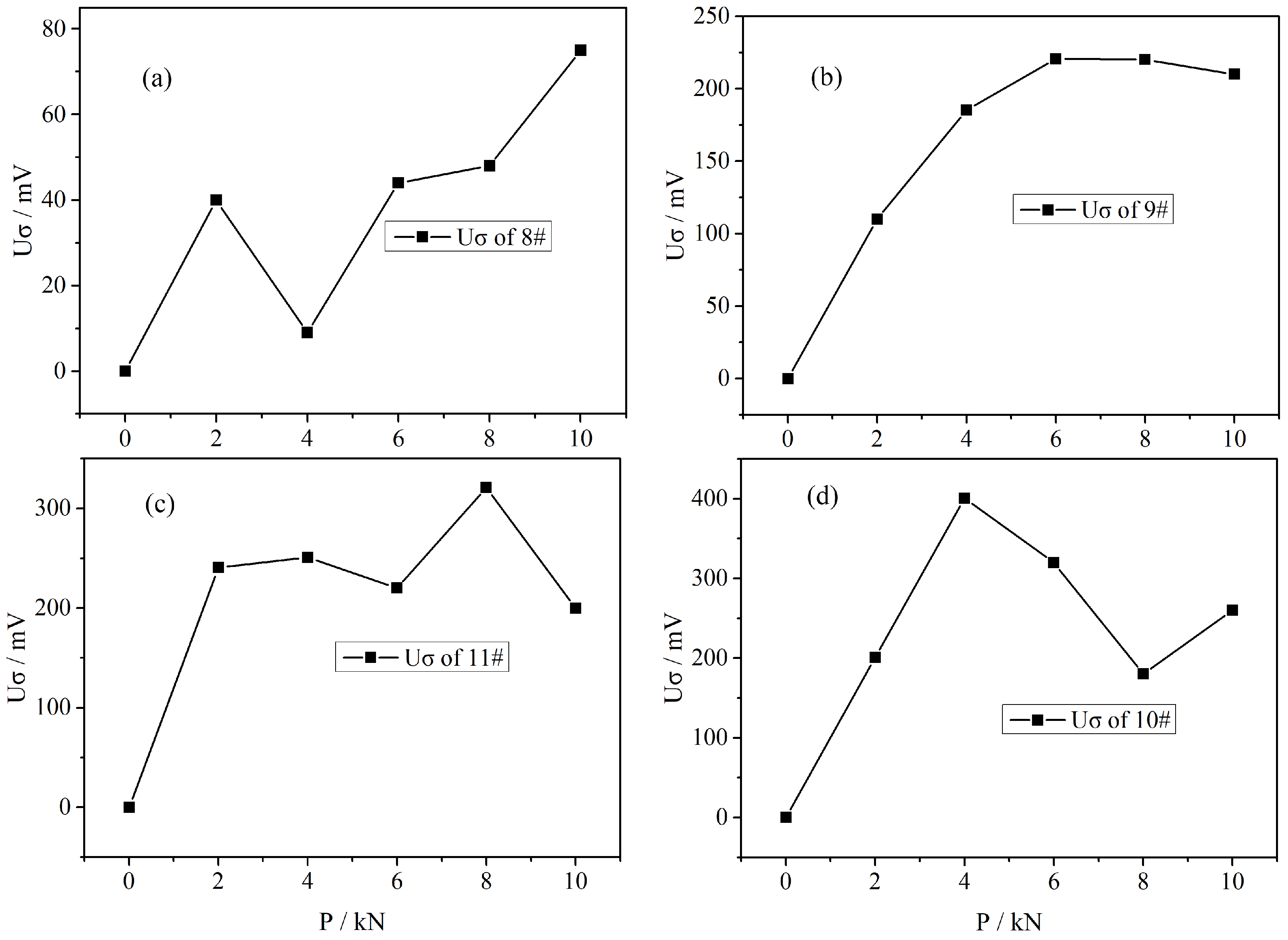
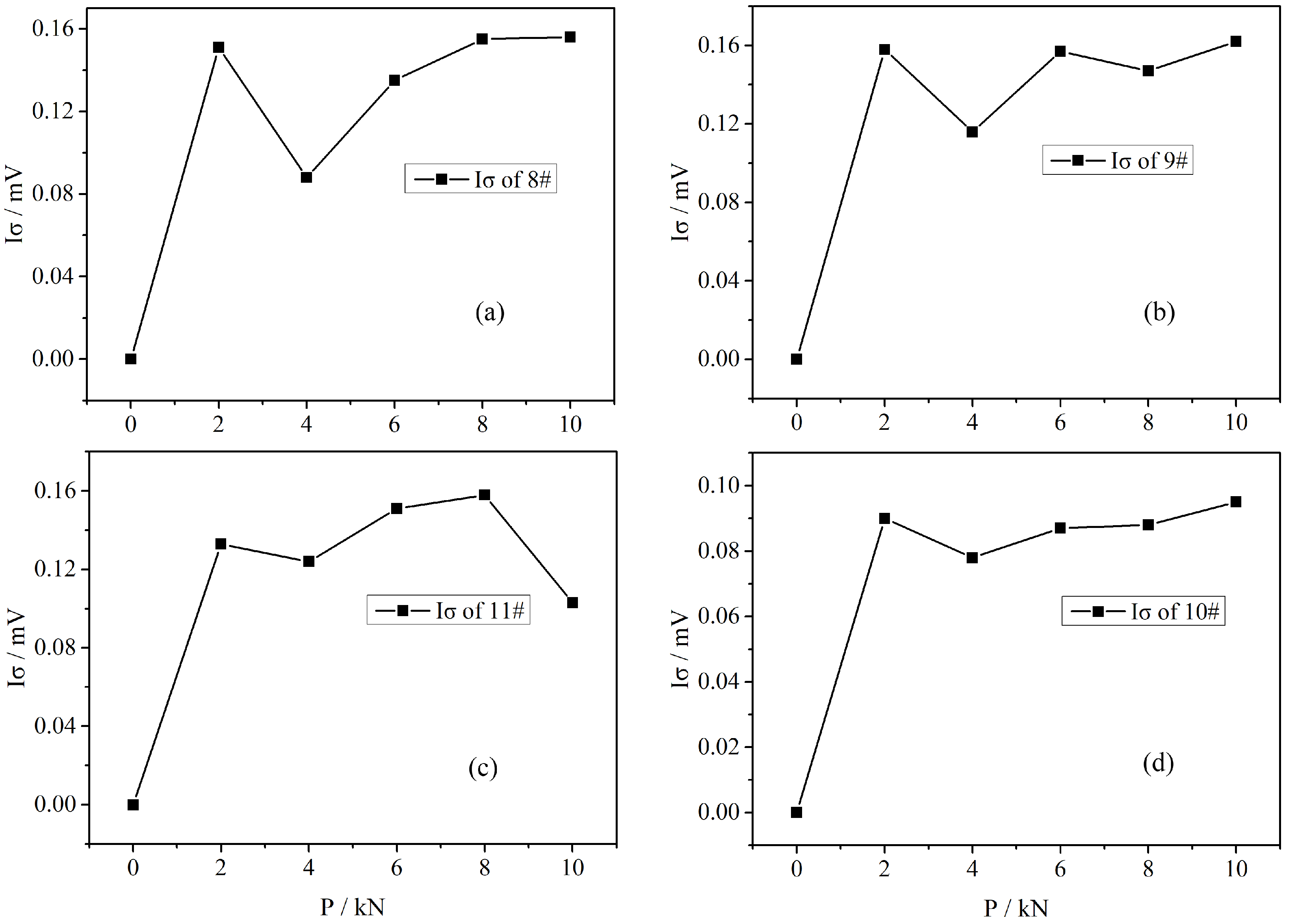
Figure 1. Schematic diagram of loading sample (1. framework of pressure testing machine; 2. loading plate; 3. insulation plate; 4. electrode; 5. sample).
Applsci 14 06474 g001
Figure 2. Physical model of loaded sample.
Applsci 14 06474 g002
Figure 3. Circuit model of piezoelectric effect.
Applsci 14 06474 g003
Figure 4. Equivalent circuit model of compressed sample.
Applsci 14 06474 g004
Figure 5. Granite sample (example image).
Applsci 14 06474 g005
Figure 6. Experimental system.
Applsci 14 06474 g006
Figure 7. Piezoelectric conversion system.
Applsci 14 06474 g007
Figure 8. Voltage waveform of granite sample 8#.
Applsci 14 06474 g008
Figure 9. A second-order circuit system composed of LCR components in series or parallel: (a) series connection of LCR components, (b) parallel connection of LCR components.
Applsci 14 06474 g009
Figure 10. Relationship between voltage (Uσ) and load (P): (a) 8# granite specimen, (b) 9# granite specimen, (c) 11# red sandstone sample, (d) 10# cement mortar sample.
Applsci 14 06474 g010
Figure 11. The relationship between current (Iσ) and load (P): (a) 8# granite specimen, (b) 9# granite specimen, (c) 11# red sandstone sample, (d) 10# cement mortar sample.
Applsci 14 06474 g011
Table 1. Measurement results of rock specimens’ physical parameters under compressive load.
Load
P (kN)
Resistance
Rσ (MΏ)
Inductance
Lσ (mH)
Capacitance
Cσ (pF)
Voltage
Uσ (mV)
Current
Iσ (mA)
Frequency
f (kHz)
 8# Granite sample
00.1710507.0000
20.131148.20474.040.00.15118.99
40.120161.40454.09.00.08818.60
60.1130.93437.044.00.135249.70
80.10713.26408.048.00.15568.44
100.10211.87401.075.00.15673.10
 9# Granite sample
00.7300104.0000
20.6814.7287.0110.10.158248.48
40.6525.0182.5185.30.116247.76
60.64141.0180.0220.70.15787.91
80.63744.8377.9220.20.14785.21
100.63352.9976.7210.00.16278.98
 11# Red sandstone sample
00.0560185.5000
20.04540.781162.0240.60.13323.13
40.03218.562060.0251.00.12425.75
60.02912.292360.0220.10.15129.56
80.02710.262843.0321.00.15829.48
100.0259.872895.0200.10.10329.78
 10# Cement mortar sample
03.940 27.0 000
23.02189.3721.0201.00.0979.85
42.89158.9419.8400.80.07889.76
62.811870.6718.9320.10.08726.78
82.751964.2018.0180.40.08826.78
102.691354.8117.0260.20.09533.18
Disclaimer/Publisher’s Note: The statements, opinions and data contained in all publications are solely those of the individual author(s) and contributor(s) and not of MDPI and/or the editor(s). MDPI and/or the editor(s) disclaim responsibility for any injury to people or property resulting from any ideas, methods, instructions or products referred to in the content.

