Abstract
When structures are subjected to dynamic loading, such as that caused by an earthquake or working machinery, the rocking behavior of objects located on parts of the loaded structure plays an important role in addressing the protection and stability of non-structural components. In this work, the free rocking of a rigid block on a flexible beam and rigid base was investigated using numerical simulations. To this end, a numerical code based on the non-smooth contact dynamics method was developed for this particular problem, and numerical simulations are compared to experimental tests when a rigid base is considered. The purpose of the study was to investigate the predictive capabilities and limitations of the numerical model and address the effect of introducing beam flexibility on the rocking response. The investigated flexibilities were such that the beam deflection under the static weight of the block remains within the common limit of 1/250 of the beam span. For a rigid base, qualitatively good correlation with the experiments was obtained, and good convergence in terms of the time-step is displayed. With the increase in beam base flexibility, it was observed that the simulation results tend to become more sensitive to mesh density and time-step size. Furthermore, we identify a limited flexibility with respect to which unreliable predictions of the overall free rocking are obtained, which corresponds to the stiffness resulting in the beam deflection under the block weight of beam-span/2500. For stiffnesses higher than that, no significant effect of beam flexibility in comparison to the rigid base was noticed in terms of tilt angle and rocking duration, which indicates the adequacy of a rigid base approximation for beams with low flexibility.
1. Introduction
In this paper, the classic problem of the rocking of a rigid block subject to an infinitesimal pulse, modeled in the seminal work of Housner [1], is generalized to rocking on a flexible structure. In engineering practice, rocking on a rigid base is important in the analysis of discontinuous structures such as graphite cores in nuclear power plants (to avoid extensive thermal stresses) [2,3] or in gravity-based traditional constructions in which no mortar or other binding agent is used, as in some monument or dry-wall structures [4]. An extensive overview of monolithic masonry walls modeled as rigid blocks on rigid foundations is provided in [5]. Controlled rocking motions are being extensively researched as a beneficial mechanism for the dissipation of seismic energy during earthquakes [6]. The principal complexity taking place in modeling rocking, regardless of whether the slipping and bouncing of the rocking body are accounted for or not, lies in its inherent discontinuity in boundary conditions. As a result, the equations of motion are not uniquely defined throughout the time domain.
After Housner’s work on pure in-plane rocking of a rigid rectangular block on a rigid base with collisions between the block and the base described by a restitution coefficient [1], a number of authors addressed rocking in a linear regime (when rotations of the block can be considered small) using an analytical approach [7,8,9,10,11]. These analyses were usually limited to simple ground motions. Some analyses were conducted using a fully nonlinear equation of motion [11,12,13]. Such a solution usually requires the use of a chosen method for the numerical integration of the equation of motion [14,15]. The restitution coefficient, which usually represents the ratio between the angular velocities immediately after and just before the impact, has been modified to improve Housner’s original assumption that the impact impulse acts at the very edge of the block [14,16,17] and takes the material dissipation into account. However, the description of rocking by an equation of motion with a single degree of freedom—the rotation of the block—cannot account for the slipping and jumping of the block [18,19], which is present in bulky blocks [12]. To tackle this, alternative approaches to modeling rocking, such as the discrete element method (DEM) [20,21] and the non-smooth contact-dynamics method (NSCD) [22], have been employed. Moreover, rocking fragility analyses for given intensity measures can be used to predict the properties of rocking motion (e.g., peak rotation angle) [23], where an intensity measure that considers excitation characteristics and geometric properties of the rigid block is proposed. Recently, the rocking of rigid blocks was also analyzed using a neural network architecture [24]. In order to protect rigid block-like structures against seismic hazards, protection methods are being developed and investigated [25].
Less investigated are problems of the rocking of rigid blocks lying on a flexible structure, although they possess substantial engineering relevance, such as marble exhibits in museums [26], non-rigidly anchored electrical cabinets in nuclear plants [27], free-standing bookshelves in libraries, furniture, or machinery that is not rigidly connected to its foundation [28]. One of the most important questions is whether the additional flexibility is beneficial or detrimental to the overall rocking stability of the block, which can represent non-structural components.
In recent years, a 3D rocking model of a block on an elastic foundation (modeled with a concentrated spring at the corners, as well as with Winkler’s spring model) was introduced in [29].
In order to deal with problems of non-smooth contact dynamics, two categories of methods have been developed over the years: event-tracking time-stepping schemes and event-capturing time-stepping schemes. Event-driven schemes [30] involve the accurate detection of events that cause discontinuities. For this reason, in more complex problems, where many different contacts may be established or the density of contacts with respect to time is high, event-driven schemes may quickly lead to time-steps in a time-integrating procedure that are far too small for the analysis to proceed with reasonable efficiency. On the other hand, event-capturing algorithms [31,32,33] turn out to be more appropriate. Effectively, these algorithms stem from the physical fact that even though an instantaneous contact force is infinitely large, its impulse is finite. In a numerical time-integration scheme necessarily involving finite time-step sizes, this naturally leads to a finite algorithmic contact force. Therefore, in event-capturing time-stepping schemes, the time-step may be kept constant throughout the simulation, even when a contact is detected, which makes them efficient and robust for complex problems involving a multitude of contact events. As originally developed, the accuracy of these algorithms is limited to the first order, which leaves ample space for further improvement, as shown, e.g., in [34,35,36]. Experiences with such advanced schemes in complex practical applications can be significantly expanded, and their performance accordingly analyzed, which leaves room for the identification of potentially needed improvements. The rocking-on-a-beam problem is representative of more complex rigid–flexible mechanical systems, for which an event-capturing algorithm is preferred.
In this work, the non-smooth contact dynamics method described in [32,33,37] is applied to the problem of a rigid block rocking on a beam structure. The simulations are performed using a code developed in Matlab, and the algorithm for the contact interaction solution is an event-capturing type of numerical scheme. For the flexible beam structure, the finite element method (FEM) is used for space discretization [38,39]. The convergence of the event-capturing algorithm employed is analyzed in terms of the block’s rotation angle, measured in laboratory experiments. The objective is to simulate a realistic scenario of a rigid body rocking on a flexible structure, which is here represented as an elastic beam. Details regarding the numerical solution procedure for this specific problem are presented. Numerical simulations are performed for a rigid and flexible beam structure. Rigid base rocking results are validated against experimental data. Possible algorithm application ranges and limitations are identified.
The studied problem is described in Section 2, which is followed by the numerical solution approach to the problem in Section 3. Details regarding the calculation of the contact forces in the setting laid out in the previous two sections are provided in Section 4. In Section 5, the experimental setup is described. In Section 6, we proceed with the experimental and numerical tests’ description, validation, and analysis. In Section 7, conclusions are drawn and future work is outlined.
2. Problem Description
In this section, the mathematical description of a rigid block rocking on an elastic beam is presented. A sketch of the problem is given in Figure 1. We start by describing the motion of the beam and block due to arbitrary loading and then the constraints imposed by contact are given.
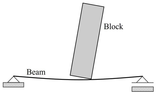
Figure 1.
Rigid block rocking on an elastic beam.
Figure 2 shows a simply supported beam of unit mass per length m, cross-sectional area A and second moment of area I, Young’s modulus E, and a damping coefficient per unit of length c, loaded with arbitrary loading in the x and y directions and . The displacements of the beam axis in the x and y directions are denoted as and . By applying Newton’s second law to an infinitesimal segment of the beam and assuming Bernoulli’s beam theory, the equations of motion for the beam are obtained as follows [40]:
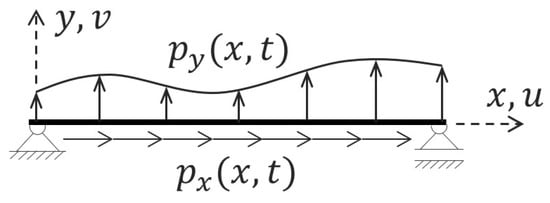
Figure 2.
Simply supported beam loaded with arbitrarily distributed loading in the x and y directions.
Figure 3a shows a rigid block at an arbitrary position in the plane. The block position is determined by the triplet , , and that represents, respectively, the x and y coordinates of the block’s centre of gravity and the rotation angle of the block. Furthermore, and denote, respectively, the x and y components of the resultant of all forces acting on the block’s centre of gravity, while is the moment with respect to the centre of gravity caused by all loads acting on the block (Figure 3b). We denote the block mass and moment of inertia as and . Now, by Newton’s second law, the equations of motion for the block are
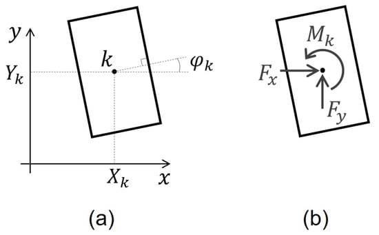
Figure 3.
(a) Block position coordinates; (b) forces acting on the block’s centre of gravity.
Regarding the contact between the block and the beam, in this work, a simplification is introduced by assuming that contact is happening only between the block vertices and the beam axis. Both normal and frictional contact are considered. Figure 4 shows the forces and developed during contact and acting on each body.
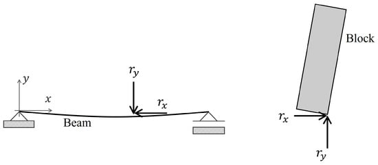
Figure 4.
Contact forces acting on the beam and block at the contact point.
We now rewrite Equations (1)–(5) including the contact forces:
For the block, the contact forces have been reduced to the centre of gravity; therefore, a moment of and with respect to the centre of gravity is added in (10) and the index k in (8) and (9) indicates the force is acting at k (Figure 3a). In the contact formulation, it is convenient to express the contact forces in a local reference frame with unit vectors and as depicted in Figure 5, in which points b and d form a contact pair. The origin of the local frame of reference is at the beam’s contact point b. The unit normal vector is normal to the beam axis at b and is directed toward the block, while the tangential axis (unit vector ) is rotated counter-clockwise with respect to and is orthogonal to .
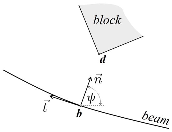
Figure 5.
Arbitrary contact pair and its local frame of reference.
In this work, a frictional contact model is used, and in order to formulate it, we need the following quantities:
- -
- g—gap function between the contacting bodies defined as , i.e., the distance between b and d;
- -
- —contact force exerted on the block by the beam expressed in the local frame, where is the normal component and is the tangential component;
- -
- —relative velocity of point d with respect to point b expressed in the local frame, with being the normal component and the tangential one.
In the non-smooth contact dynamics method [32] used in this work, it is assumed that there is no penetration between the block and the beam, the contact force is repulsive, and when the bodies are not in contact, the contact force equals zero.
All this is encompassed with the following set of unilateral constraints, known as the Signorini condition [32]:
When contact with deformable bodies is concerned, the contact constraint can be formulated at the velocity level [41]:
where is the normal component of the velocity immediately after impact. Condition (12) is referred to as the velocity Signorini condition. In order to complete the model, an impact law is necessary. Newton’s impact law can be used, which relates the normal velocity just before the impact to the velocity just after the impact as , where e is the coefficient of restitution ranging from 0 to 1, and is the velocity immediately before impact. In this work, the impact is assumed to be plastic, which implies a value of , and the velocity Signorini condition is used. To account for frictional forces, the Coulomb law is used, which states the following:
where is the coefficient of friction and is the relative tangential velocity of d with respect to b during contact. From the last two equations, we see that has a limiting value and its direction is opposite to the sliding velocity.
3. Numerical Solution
In this section, the numerical procedure for the solution of the equations of motion and the discrete form of the Signorini conditions are laid out. We then outline how to obtain the mean impulse of the contact force.
3.1. Beam Space Discretization
The equations of motion of the beam are fourth-order partial differential equations in which the unknown functions, displacement u and v, are functions of space and time. The solution of those equations is obtained by the finite element method (FEM). The finite element form of (7) and (6) involves transforming the equations into their weak form, splitting the domain into smaller segments (finite elements) and introducing approximation functions for the displacement fields. This procedure leads to a set of ordinary differential equations with respect to time, which is written in a matrix form as
For more details, the reader can refer to [38,39]. In the equation above, is the mass matrix, is the damping matrix, is the stiffness matrix, is the vector load, and is the vector of contact forces, and they all appertain to the beam. Within the finite element method, the displacements of the nodal points are obtained. The vectors , and collect, respectively, the displacements, velocities, and accelerations of the nodal points, which are obviously functions of time. For the analysed beam, each node of the beam has three displacement components (or degrees of freedom) [42], namely, the displacements in the x and y directions and a rotation.
3.2. Time Integration
The time integration of the equations of motion of the whole system is performed as proposed in [32], where the method [43] was used for integrating the equations of motion. First, the equations of motion for the block (8)–(10) are rewritten in matrix form:
where
The motion of the block is described by the position vector and its derivatives with respect to time are denoted by the dots over the vector. In the equations above, is the block mass matrix, is the acceleration vector, is the vector of external loads, and is the vector of the contact force. The index k indicates a reference to the block.
We consider some arbitrary time interval of length . Integrating (16) over , the velocity at the end of the time interval follows as
The position at is evaluated as
Hereafter, approximations of all quantities at time instants and are referred to through the indices i, and , e.g., , , and so on.
The contact force variation with time is unknown; therefore, only the impulse of the force is calculated. More precisely, in contact dynamics, the mean value of the impulse is sought:
which basically corresponds to a constant contact force over the interval , and therefore, we refer to it as the contact force. Applying the method in (18) and (19) results in discretized expressions for the velocity and position at
where is some parameter between 0 and 1. With (21) and (22), an approximate discrete solution for the block position is obtained.
For the beam, we repeat the procedure. We integrate (15) and approximate the integrals with the method, which gives
Now, after approximating the positions at , and grouping all the terms with on the left side of the equation, the approximate velocities and positions at the end of the time-step are
In (24), is
Equations (21), (22), (24) and (25) can be collected together and written in the following way:
with
Equations (27) and (28) describe the motion of the entire system consisting of the block and the beam structure. The displacement vector for the entire system is , and is the vector of all forces. The first two terms on the right-hand side of (27) represent the velocity at the next time-step when there is no contact force, and by denoting this velocity as , (27) is rewritten as
3.3. Discrete Form of the Contact Constraints
As already mentioned, the constraints induced by the contact are taken into account through the velocity Signorini conditions (12). Based on the non-smooth contact dynamics method, for a discrete model, the velocity Signorini conditions are
The above conditions can be also written in the following form:
Coulomb law follows as
4. Contact Force Calculation
Contact forces are calculated when a contact is detected. That means that for each time instant a check if the bodies overlap is performed. When overlapping (contact) is detected, a contact pair is determined, and the local frame of reference is set up (see Figure 5). The contact pair is a set of two points that will touch each other when contact occurs.
We first analyze the case when a contact takes place only at one point as in Figure 5. The contact force is calculated by determining its normal () and tangential () components in a local frame of reference. To this end, we need the velocity of the block’s vertex d relative to the contact point b on the beam (see Figure 5). To obtain the relative velocities and forces in the local frame, a transformation matrix is used to provide
By applying transformation matrix , an equation relating the relative velocities and contact forces of the contact pair is obtained:
where
in which defines a position of the system at some instant within the interval . Equation (41) is used to calculate the contact forces. Conditions (12) then imply . The value of is initially assumed to be zero, implying sticking contact conditions. Now with equation (41) allows us to proceed with the evaluation of the contact forces. In this process, the Coulomb law is considered, from which we can tell if contact is of the sticking or sliding type, and the value of the tangent contact force is determined accordingly. This involves checking if remains below its limit value, in which case sticking contact takes place; otherwise, the value of is set to its limit and (sliding) takes place.
The solution for contact forces is provided in [32,44].
When several contacts occur simultaneously, more impulse forces act at the same time and (41) takes the following form:
where h refers to a particular contact and j refers to all other remaining contacts. In this case, the solution is looked for iteratively. For each iteration, every contact is solved according to (44) in which the previously obtained values for the other contact forces are used. This procedure is repeated until newly obtained values of the contact forces do not change from the previous more than a predefined amount. Details about this procedure are provided in [32]. For the beam-block problem, a maximum of two simultaneous contacts can occur (assuming contact only at block vertices) and the solution is obtained by using (44) as described.
4.1. Transformation Matrix
For the block it was said that only its vertices are assumed to contact with the beam. An arbitrary vertex d is considered as shown in Figure 6, where the block at some arbitrary position and with some rotational velocity is depicted. We denote the angle between the x axis (of the global reference frame) as and the velocity vector of point d caused only by the block’s rotational velocity , as shown in Figure 6, while the block’s half diagonal is s. The velocity of some vertex d is given as
or in compact form
In order to be able to evaluate at any instant, we first evaluate it at some reference position, here taken to be at and for . Under these conditions, for each vertex is shown in Figure 6b. Now, for any vertex can be evaluated at each instant in time as
and the vertex velocity given in (45) can be determined.
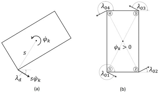
Figure 6.
(a) Arbitrary position of the block with some rotational velocity ; (b) angles of the velocity vectors at the block vertices caused only by block rotation at the reference configuration .
To express the vertex velocity in a local reference frame , we will use the transformation matrix that expresses vectors from the global reference frame to the local frame:
where is the angle between the local and global reference frame as shown in Figure 5. The inverse transformation, i.e., from local to the global reference frame, is given by the inverse of , which equals its transpose because is orthogonal. Now, the velocity of vertex d in local coordinates is
where
The normal and tangential components in the local frame are, respectively, denoted as and .
The velocity of an arbitrary point b on some finite element a of the beam is given as
where () are the velocities of nodal displacements of the finite element. In a compact form, we write (52) as
Expressing this velocity in a local frame, we obtain
where and are given as
and denote the normal and tangential components of the velocity of point b, respectively. Now, having obtained the velocities in the local frame, we can express the relative velocity as the difference between the block and beam contact point velocity. We drop the time variable below for simplicity reasons. The components of the block vertex velocity relative to the beam point in the local frame are obtained by subtracting their velocities in the local frame:
which, by making use of (49) and (54), yields
where is the relative velocity in the normal direction and is the relative velocity in the tangential direction. By knowing the transformation from global velocities to local relative velocites, the opposite transformation, i.e., the form of global to local velocities, is given as and is used to obtain global contact forces from the impulse forces in the local frame.
4.2. Contact Pair Detection
In order to define the local reference frame shown in Figure 5, the point on the beam contacting with the block has to be determined. Let us assume that during the evaluation of the positions at the new time-step, the bodies overlap, as shown in Figure 7. The block vertex d is identified as the contact point on the block and forms one element in the contact pair. The contact point on the beam is chosen to be the point closest to vertex d in the considered configuration.
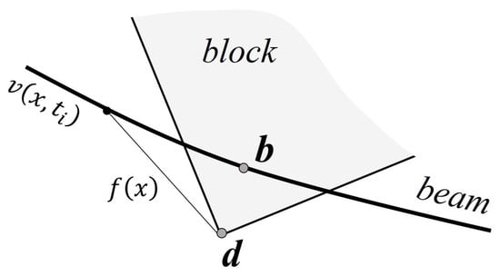
Figure 7.
Enlarged sketch of the block and beam in an overlapping configuration: —beam deformed axis; b—point of contact on the beam; d—block vertex that impacts the beam; —distance between vertex d and beam axis.
This means that the point on the beam closest to the block vertex d has to be found. In order to do so, we need the distance function between the beam and block vertex d whose position is known.
The displacement of the beam is given as
which, for the Euler–Bernoulli beam, is a third-degree polynomial. Labels with are the local degrees of freedom of the beam element considered. Now, by denoting the x and y coordinates of vertex d as the distance function between the vertex d and the beam displacement curve is given as
where is the beam displacement function at some instant . The distance function given in (60) will have its minimum value at the coordinate x that corresponds to the point on the beam that is nearest to vertex d:
which gives
Equation (62) is a fifth-degree polynomial, and its roots are computed numerically using a Matlab built-in function. After finding the roots, the real values are inserted into the distance function and the root giving the minimal value of is chosen as the x coordinate of the contact point b, denoted hereafter as , i.e., the coordinates of b are . It is also required that the contact point lies between the beam nodes , where and are the x coordinates of the beam nodes. If this condition is not satisfied, then the contact search is performed on the corresponding neighboring element. Once the contact pair is determined, the local reference frame inclination angle is evaluated as
5. Experimental Setup
In order to validate the developed numerical algorithm, an experimental program focused on measuring the free rocking response was designed and conducted. All the experiments were conducted in the Structural Laboratory of the Faculty of Civil Engineering in Rijeka. The experimental setup is shown in Figure 8. Each block was initially tilted at an angle of and released from rest in such a position (Figure 8b). This followed the procedure previously suggested by Čeh et al. [14]. The rocking response was monitored by a contactless optical measuring system ZEISS Aramis 4M (ZEISS, Baden-Württemberg, Germany), with two cameras, each with resolution 2400 × 1728 pixels, and a measuring frequency of 150 fps (Figure 8a).
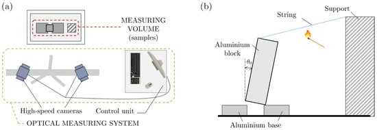
Figure 8.
Experimental setup: (a) top view of the optical measuring system and measuring volume, (b) front view of the measuring volume.
The experiment is performed on a rigid base to focus entirely on validating the contact treatment in the developed algorithm, without introducing the effects of the elasticity of the beam. Therefore, the experimental validation is performed for the case when the base in the numerical code is rigid, which was obtained by setting the beam Young modulus to a high value.
The mass and dimension of the tested blocks are given in Table 1. Each block has a rectangular base of dimensions b × b, mass m, height h, angle between the block’s vertical edge, and the diagonal and length of the semi-diagonal s. The rocking of a block was physically constrained so that only the rotation of the block was possible, while any sliding and/or jumping of the block was prevented (as shown in Figure 9a, according to [14]). This was obtained by using tape strips, marked with blue and green in Figure 9a, which are attached to the block and base. The tape strips do not allow the slipping of the block in the x direction, but since they posses no flexural stiffness rotation is allowed.

Table 1.
Geometric characteristics and masses of the tested blocks.
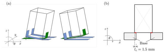
Figure 9.
Experimental setup according to [14]: (a) system of tapes to assure pure rocking, (b) edge contact between the base and the block.
Since the developed algorithm assumes a contact point between the bodies, the experiment were designed so that the contact between the block and the body beneath it occurs along 1.5 mm of the surface near the block’s edge. In this way, the assumption used in the algorithm is validated.
6. Results and Discussion
In this section, we investigate if a correlation between rocking on a rigid and flexible base exists. First, the case of rocking on a rigid base is presented, for which convergence analyses and experimental validations are performed. Then, the base flexibility is gradually increased and its influence on rocking and on the algorithm predictions is tested. In that process, the influence of mesh density and time-step size are checked. Moreover, comparisons between the numerical predictions of free rocking on a flexible beam and rocking on a rigid base are provided.
The structural base on which the block is rocking is implemented as a simply supported beam. For this type of boundary conditions, the simplification that contact is happening only at the block vertices adequately represents the real case since the beam will bend downward in a convex shape. Other boundary conditions and complex loading excitations could require the generalization of the contact algorithm in order to model more generic contact conditions, such as contact occurring between the block edge and beam. In all examples, it is assumed that the beam has a span of 30 cm, cross-section width and height of 40 mm and mm, respectively, Poisson’s ratio of , and density of . In order to introduce damping effects, as they are present in real structures, Rayleigh damping was used, with the values of damping ratios (for the first natural frequency) and (for the third natural frequency) [42,45]. The friction coefficient was set to . This value was obtained as an average from several simple tests involving a block laying on a beam. The beam was initially in a horizontal position, and then its inclination was gradually increased until the sliding of the block occurred. The inclination angle at which the block starts to slide was measured, and the coefficient of friction is obtained as the tangent of this angle. The weight of the beam is taken into account throughout the simulation, and the beam is given an initial displacement under its own weight and the block’s weight, which corresponds to the actual initial conditions. For time integration, the -parameter was set to 1, leading to the backward Euler method. The block material and geometry characteristics are reported in Table 1. The Young’s modulus value is provided in the specific examples since the value is varied in order to change the bending stiffness of the beam structure. All analyzed stiffnesses are such that the beam displacement caused by the block weight is less than of the beam span. This value is chosen in accordance with most building codes that limit the maximum value of the deflection as to of the span length [46]. Moreover, this limitation justifies the application of linear beam theory that has been implemented in the numerical code. Nonetheless, we point out that the NSCD approach can be applied also to problems in which large displacements and deformations occur [32].
6.1. Convergence Analysis
Convergence analyses regarding the time-step and mesh density are performed for the block rocking on a rigid base. The rigid base is obtained by setting the beam Young’s modulus to a very high value, in this case taken to be equal to Pa. The block’s initial conditions are set to be equal to the experimental ones for the B6M block (which will be presented in the following section). In Figure 10, the results of four simulations with different time-steps ranging from s to s are shown. It is observed that convergent behaviour is displayed as the time-step is decreased. With time-steps s and smaller, no significant change in the block behaviour (in terms of block rotation) is observed. The time-step s appears to be too large, causing the results to differ from the smaller time-steps after approximately s. A time-step of s is chosen for the following analyses.
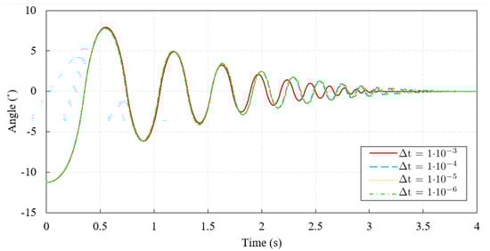
Figure 10.
Analysis of the influence of time-step size on the rocking response.
In Figure 11, results from simulations with different beam FEM meshes, composed of 3, 6 and 12 elements, are shown. No difference is observed in the results between the meshes. We point out that due to the code architecture, the block should not touch the two elements at the ends, and therefore, the mesh of 6 elements is used in further analyses.
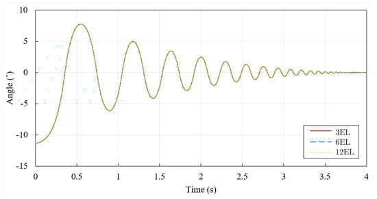
Figure 11.
Analysis of the influence of FEM mesh density on the rocking response.
6.2. Free Rocking on a Rigid Base
Based on the previously performed convergence tests, herein, the mesh of six elements and the time-step of s are used. In each test, an arbitrary inclination angle is chosen since it has no significant influence on the rocking behaviour, and the reported value was measured from the experiment’s initial conditions. Obviously, it was considered that the initial angle does not exceed the value , in which case immediate overturning would occur. First, we consider the example involving block B6M with a slenderness ratio of 4.5, which corresponds to slender rocking bodies. In the initial configuration, the block is inclined around one of its corners touching the base at an angle of −11.268° with respect to the stable vertical position and is released from rest and left to move under the action of gravitational force.
Rotation time histories obtained experimentally and numerically are given in Figure 12. It can be seen that after the first impact, a delay is present in the numerical result with respect to the experimentally obtained ones. The experimentally measured block angle after the first impact was −6.92°, while the simulation predicted an angle of −7.76°. Nonetheless, good overall behaviour is predicted by the simulation, in terms of both tilt amplitude and decay. Both time histories reach a rest state around 3.5 s. The corresponding angular velocity time histories for this block are shown in Figure 13, and observations similar to the ones made for the block angle can also be noticed when analyzing angular velocities.
Since an slenderness ratio equal to 4 is usually taken as the limit to considering slender rocking bodies, the analysis of block B6M () is complemented by an analysis of two additional blocks: one considered bulky (block B3M with ), and one considered significantly slender (block B8M with ).
Figure 14 gives a comparison between numerical and experimental results for the block with the smallest slenderness ratio —. The initial rotation angle is −14.839°. This block is considered bulky, and inverted-pendulum-based models (e.g., Housner’s [1]) are considered unable to simulate its behaviour accurately enough. From Figure 14, we can notice that the overall time history of the block rotation angle is qualitatively well predicted by the numerical analysis. The smaller number of vertex impacts is successfully predicted. In the simulation, a faster decrease in the rocking period (the time between two impacts at each rocking half-cycle) is obtained with respect to the experiment. The numerically predicted block rotation angle is similar to the one measured in the experiment; they are, respectively, −8.28° and −8.35°.

Figure 12.
Block B6M—experimental and numerical results for the block rotation angle in time.
Figure 12.
Block B6M—experimental and numerical results for the block rotation angle in time.


Figure 13.
Block B6M—experimental and numerical results for the block angular velocity in time.
Figure 13.
Block B6M—experimental and numerical results for the block angular velocity in time.


Figure 14.
Block B4M—experimental and numerical results for the block rotation angle in time.
Figure 14.
Block B4M—experimental and numerical results for the block rotation angle in time.

The last block from the experimental campaign is the B8M block. This is the most slender of the three, and therefore, it exhibits shorter rocking periods, as can be seen in Figure 15. The initial rotation angle was −7.731°. For this example, differences start to appear already after the first impact (somewhere around 0.5 s), with the simulation predicting a maximum angle of −6.18° after the first impact, while in the experiment, an angle of −5.16° was measured. The delay of the numerical results with respect to the experiment increases with time. However, we can note that the overall behaviour is predicted well, particularly the decay rate of the inclination angle when a larger number of impacts occur.
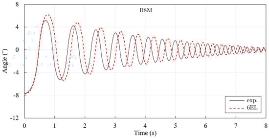
Figure 15.
Block B8M—experimental and numerical results for the block rotation angle in time.
Based on this analyses, we take the elastic modulus value of Pa as the reference value corresponding to a rigid base, since good time-step convergence was obtained (at s) and the mesh was not sensitive to the analysis.
In order to ensure that no slipping was happening, as was the case in the experiments, test simulations with friction coefficients of 0.7 and 1.0 were run, and no effect on the simulation results was observed. For this reason, the value initially chosen () was kept throughout all the analyses.
6.3. Free Rocking on a Flexible Beam Structure
Numerical results for the elastic beam structure are presented and discussed. The goal is to investigate the effect of beam flexibility on the rocking of the block and on the numerical algorithm’s prediction capability. The effect of beam flexibility on the rocking response is also analyzed by comparing it with the rocking on a rigid base; therefore, the experimental results for the rigid base rocking are also displayed in the following figures together with the numerical results.
We will refer to as the Young’s modulus for which the beam deflects for L/2500 under the block’s weight concentrated at the beam centre. Young’s modulus in the following analyses is set as , where n is varied in order to change the beam’s bending stiffness. The geometrical characteristics of the beam and all other material properties used in the model are provided at the beginning of Section 6. Figure 16 shows a set of simulations where the mesh and time-step from the rigid base model are kept while increasing the flexibility of the beam (i.e., reducing its Young’s modulus). It is observed that as the flexibility is increasing, the numerical predictions start to differ, in particular when the stiffness drops from to .
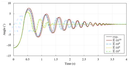
Figure 16.
Block angle time history for flexibility increase in the rigid base model.
In Figure 17, the time interval containing the first two impacts from Figure 16 is extracted. It can be seen that differences start to appear after the impacts between the block and the beam base. Since the mesh discretization and time-step are unchanged, it can be observed that the impulse occurring during contact is also affected by the beam stiffness.
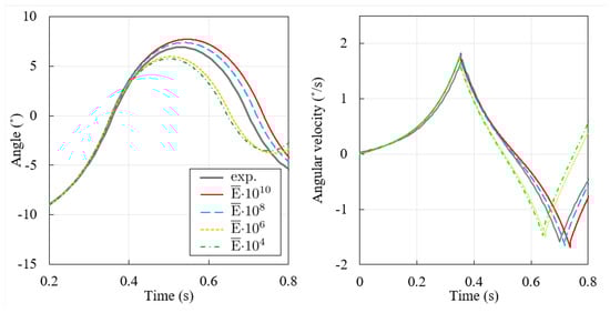
Figure 17.
Zoomed image of the block rotation angle between the first two impacts.
In the following, mesh and time-step effects on the numerical results are analyzed. Figure 18 shows the results obtained with different meshes. It is observed that the mesh initially displays fast convergence, while for flexibility obtained with , the prediction of the block’s rotations becomes sensitive to the mesh.
A similar observation is made by analyzing the time-step effect in Figure 19, but the time-step influence can be noticed for much higher bending stiffness (already for ). A decrease in the time-step shows a convergent trend for all analyzed values of Young’s modulus until , but it appears that rather small time-steps become necessary. However, the simulations clearly indicate that the rocking behaviour still qualitatively replicates rocking on a rigid base, i.e., smooth decay of the rotation angle until a rest state is reached and a similar time to reach it. This trend appears to happen up to the stiffness corresponding to a deflection of under the block weight, where L is the beam span. The value corresponds to the engineering limit for beam deflection in structures.

Figure 18.
Mesh density effect on the rocking behaviour when increasing the flexibility.
Figure 18.
Mesh density effect on the rocking behaviour when increasing the flexibility.

For further increases in flexibility, it was observed that convergence is lost after a few impacts, both in terms of mesh and time-step, as shown in the last graph of Figure 19. This is observed for the beam with stiffness giving a static displacement under the block weight of roughly . Therefore, below this limit, the predictions do not provide convergent and reliable results for the entire simulation time.


Figure 19.
Time-step size effect on the rocking behaviour when increasing the beam flexibility.
Figure 19.
Time-step size effect on the rocking behaviour when increasing the beam flexibility.


7. Conclusions
In this work, the non-smooth contact dynamics (NSCD) method was applied in a numerical procedure for simulating the rocking of a rigid block on an elastic beam structure. An in-house numerical code was developed using the finite element method (FEM) to discretize the beam, the NSCD approach to solve the contacts between the block and the beam, and the method for time-stepping. Governing equations for the specific application and constraint conditions are summarized. Details about the transformation matrices, which required in NSCD to obtain relative velocities and impulse force in the local frame of reference, are provided for the investigated problem. Furthermore, the procedure for the detection of contact points is presented. Rocking of a rigid block on top of a non-rigid beam was investigated using a combined numerical-experimental approach. A focused experimental program aimed at a detailed investigation of free rocking was conducted using contactless measuring equipment and a digital image correlation approach. Numerical performance regarding the application of NSCD to the aforementioned problem was investigated. The convergence properties were tested and the capability to reproduce experimental tests were validated.
In the analysis of rocking on a rigid base, three blocks with different slenderness were analyzed, and numerical data were compared against experimental tests. Predictions of the block rotation angle by the simulations were observed to qualitatively reproduce the trend of rotation time histories recorded in the experiments under the same initial conditions. A similar decay of rotation angle and actual values of the angle were observed. However, most of the simulations exhibited a shift in the time history of the block rotation angle, which becomes noticeable for a higher number of impacting contacts.
The effect of the flexibility of the base structure on the rocking and on the predictive capabilities of the algorithm was investigated by gradually introducing flexibility into the beam. This was carried out simply by decreasing the value of Young’s modulus. The analyses showed that as the beam structure becomes more elastic the effect of the time-step and mesh density on the results increases. However, it is shown that up to the stiffness of , the mesh density has little effect on the results (mesh convergence is rapidly reached), and a convergent trend for the time-step is displayed. Up to this limit, the simulations indicate that block rotation is qualitatively very similar to rocking on a rigid base, meaning that the beam has negligible influence on the block’s stability during the free rocking regime, and rigid base approximations could be applied for such cases. With further flexibility, an increase the effect of both the time-step and mesh density on the rocking response becomes more significant, and the algorithm does not reach convergence. When beam flexibility is such that the block’s weight causes a static displacement of 1/2500 of the beam span, convergence is lost, and the results of the numerical procedure become different and unpredictable. The divergence in results starts after just a few impacts of the block with the beam. This indicates that the next steps should aim at improving the numerical algorithm in order to successfully simulate systems with beams of lower stiffness, complemented with appropriate experimental validation.
All of the performed analyses provide insight into the predictive capability of the numerical NSCD method when applied to a specific problem concerning the free rocking of a rigid block, both on a rigid base and on an elastic beam structure.
Further work will involve investigations of and improvements to the NSCD procedure applied herein in order to accurately reproduce the rocking motion on a more flexible structure. Moreover, experimental testing for rocking on flexible structures would provide insight into the block behaviour and benchmark data for numerical validations.
Author Contributions
T.M.: conceptualization, methodology, software, validation, formal analysis, investigation, writing—original draft preparation, writing—review and editing, funding acquisition. N.Č.: conceptualization, methodology, formal analysis, data curation, investigation, writing—original draft preparation, writing—review and editing, funding acquisition. S.H.: methodology, software. M.A.: writing—review and editing, supervision, project administration, funding acquisition. All authors have read and agreed to the published version of the manuscript.
Funding
This research was conducted as a part of the projects Parameter analysis and calibration for the numerical modeling of a rigid block rocking on an elastic beam—the non-smooth contact dynamics approach (uniri-mladi-tehnic-22-72 2859) and Dynamic characterisation of rigid blocks with cohesive contacts (uniri-iskusni-tehnic-23-280 3274) and financially supported by University of Rijeka, as well as the project Joint Training on Numerical Modelling of Highly-flexible Structures for Industrial Applications—THREAD (Horizon2020 MSCA No. 860124), which was financially supported by an EU commission. Experimental investigation was carried out within a bilateral collaboration Rigid body rocking on a flexible structure—non-smooth contact-dynamics approach and experimental validation and Integration schemes with fixed time step size for non-smooth dynamical systems with contact and friction between University of Rijeka, Faculty of Civil Engineering (Croatia) and Martin-Luther-University Halle-Wittenberg (Germany), Institute of Mathematics, supported by Croatian Ministry of Science and DAAD—Deutscher Akademischer Austauschdienst.
Institutional Review Board Statement
Not applicable.
Informed Consent Statement
Not applicable.
Data Availability Statement
The original contributions presented in the study are included in the article, further inquiries can be directed to the corresponding author.
Acknowledgments
The authors whish to thank Gordan Jelenić for his valuable discussions and insights.
Conflicts of Interest
The authors declare no conflicts of interest.
References
- Housner, G.W. The behavior of inverted pendulum structures during earthquakes. Bull. Seismol. Soc. Am. 1963, 53, 403–417. [Google Scholar] [CrossRef]
- Dihoru, L.; Crewe, A.; Taylor, C.; Horgan, T. Shaking Table Experimental Programme; Technical Report; Aston University: Birmingham, UK, 2011. [Google Scholar]
- Voyagaki, E.; Kloukinas, P.; Dietz, M.; Dihoru, L.; Horseman, T.; Oddbjornsson, O.; Crewe, A.J.; Taylor, C.A.; Steer, A. Earthquake response of a multiblock nuclear reactor graphite core: Experimental model vs simulations. Earthq. Eng. Struct. Dyn. 2018, 47, 2601–2626. [Google Scholar] [CrossRef]
- Smoljanović, H.; Živaljić, N.; Nikolić, Ž.; Munjiza, A. Numerical Simulation of the Ancient Protiron Structure Model Exposed to Seismic Loading. Int. J. Archit. Herit. 2021, 15, 779–789. [Google Scholar] [CrossRef]
- Casapulla, C.; Giresini, L.; Lourenço, P.B. Rocking and Kinematic Approaches for Rigid Block Analysis of Masonry Walls: State of the Art and Recent Developments. Buildings 2017, 7, 69. [Google Scholar] [CrossRef]
- Makris, N. A half-century of rocking isloation. Earthquakes Struct. 2014, 7, 1187–1221. [Google Scholar] [CrossRef]
- Makris, N.; Zhang, J. Rocking Response and Overturning of Anchored Equipment under Seismic Excitations; Pacific Earthquake Engineering Research Center, University of California: Berkeley, CA, USA, 1999. [Google Scholar]
- Shi, B.; Anooshehpoor, A.; Zeng, Y.; Brune, J.N. Rocking and overturning of precariously balanced rocks by earthquakes. Bull. Seismol. Soc. Am. 1996, 86, 1364–1371. [Google Scholar] [CrossRef]
- Smoljanović, H.; Živaljić, N.; Nikolić, Ž. A combined finite-discrete element analysis of dry stone masonry structures. Eng. Struct. 2013, 52, 89–100. [Google Scholar] [CrossRef]
- Spanos, P.D.; Koh, A.S. Rocking of rigid blocks due to harmonic shaking. J. Eng. Mech. 1985, 110, 1627–1642. [Google Scholar] [CrossRef]
- Zhang, J.; Makris, N. Rocking Response of Free-Standing Blocks under Cycloidal Pulses. J. Eng. Mech. 2001, 127, 473–483. [Google Scholar] [CrossRef]
- Dimitrakopoulos, E.; DeJong, M. Overturning of Retrofitted Rocking Structures under Pulse-Type Excitations. J. Eng. Mech. 2012, 138, 936–972. [Google Scholar] [CrossRef]
- Makris, N.; Konstantinidis, D. The Rocking Spectrum and the Shortcomings of Design Guidlines; Technical Report; University of California: Berkeley, CA, USA, 2001. [Google Scholar]
- Čeh, N.; Jelenić, G.; Bićanić, N. Analysis of restitution in rocking of single rigid blocks. Acta Mech. 2018, 229, 4623–4642. [Google Scholar] [CrossRef]
- Čeh, N.; Jelenić, G. Numerical and experimental investigation of rocking stability of rigid blocks during single sine-wave excitation. Eng. Rev. 2022, 42, 149–162. [Google Scholar] [CrossRef]
- Kalliontzis, D.; Sritharan, S.; Schultz, A. Improved Coefficient of Restitution Estimation for Free Rocking Members. J. Struct. Eng. 2016, 142, 6016002. [Google Scholar] [CrossRef]
- Chatzis, M.N.; Garcia Espinosa, M.; Smyth, A.W. Examining the Energy Loss in the Inverted Pendulum Model for Rocking Bodies. J. Eng. Mech. 2017, 143, 4017013. [Google Scholar] [CrossRef]
- Ishiyama, Y. Motions of Rigid Bodies and Criteria for Overturning By Earthquake Excitations. Earthq. Eng. Struct. Dyn. 1982, 10, 635–650. [Google Scholar] [CrossRef]
- Sinopoli, A. Earthquakes and large block monumental structures. Ann. Geofis. 1995, XXXVIII, 737–751. [Google Scholar] [CrossRef]
- Winkler, T.; Meguro, K.; Yamazaki, F. Response of rigid body assemblies to dynamic excitation. Earthq. Eng. Struct. Dyn. 1995, 24, 1389–1408. [Google Scholar] [CrossRef]
- Andreaus, U.; Casini, P. On the rocking-uplifting motion of a rigid block in free and forced motion: Influence of sliding and bouncing. Acta Mech. 1999, 138, 219–241. [Google Scholar] [CrossRef]
- Zhang, H.; Brogliato, B. The Planar Rocking-Block: Analysis of Kinematic Restitution Laws, and a New Rigid-Body Impact Model with Friction de Recherche; Inria: Le Chesnay-Rocquencourt, France, 2011. [Google Scholar]
- Liu, H.; Huang, Y.; Liu, X.; Yu, X.; Su, J.; Zhang, X.; Liu, H.; Huang, Y.; Liu, X. An Intensity Measure for the Rocking Fragility Analysis of Rigid Blocks Subjected to Floor Motions. Sustainability 2023, 15, 2418. [Google Scholar] [CrossRef]
- Banimahd, S.A.; Giouvanidis, A.I.; Karimzadeh, S.; Lourenço, P.B. A multi-level approach to predict the seismic response of rigid rocking structures using artificial neural networks. Earthq. Eng. Struct. Dyn. 2024, 53, 2185–2208. [Google Scholar] [CrossRef]
- Basili, M.; De Domenico, D.; Di Egidio, A.; Contento, A. Improvement of the Dynamic and Seismic Behaviour of Rigid Block-like Structures by a Hysteretic Mass Damper Coupled with an Inerter. Appl. Sci. 2022, 12, 11527. [Google Scholar] [CrossRef]
- Yim, C.S.; Chopra, A.K.; Penzien, J. Rocking Response of Rigid Blocks to Earthquakes. Earthq. Eng. Struct. Dyn. 1980, 8, 565–587. [Google Scholar] [CrossRef]
- Cho, S.G.; Salman, K. Seismic demand estimation of electrical cabinet in nuclear power plant considering equipment-anchor-interaction. Nucl. Eng. Technol. 2022, 54, 1382–1393. [Google Scholar] [CrossRef]
- Aslam, M.; Scalise, D.T.; Godden, W.G. Earthquake Rocking Response of Rigid Bodies. J. Struct. Div. 1980, 106, 377–392. [Google Scholar] [CrossRef]
- Chatzis, M.; Smyth, A. Modeling of the 3D rocking problem. Int. J. Non. Linear. Mech. 2012, 47, 85–98. [Google Scholar] [CrossRef]
- Pfeiffer, F.; Glocker, C. Multibody Dynamics with Unilateral Contacts; John Wiley & Sons: Hoboken, NJ, USA, 1996. [Google Scholar] [CrossRef]
- Acary, V. Projected event-capturing time-stepping schemes for nonsmooth mechanical systems with unilateral contact and Coulomb’s friction. Comput. Methods Appl. Mech. Eng. 2013, 256, 224–250. [Google Scholar] [CrossRef]
- Jean, M.; Jean, M. The non-smooth contact dynamics method. Comput. Methods Appl. Mechan-Ics Eng. 1999, 177, 3–4. [Google Scholar] [CrossRef]
- Moreau, J.J. Numerical aspects of the sweeping process. Comput. Methods Appl. Mech. Eng. 1999, 177, 329–349. [Google Scholar] [CrossRef]
- Acary, V. Higher order event capturing time-stepping schemes for nonsmooth multibody systems with unilateral constraints and impacts. Appl. Numer. Math. 2012, 62, 1259–1275. [Google Scholar] [CrossRef]
- Schindler, T.; Rezaei, S.; Kursawe, J.; Acary, V. Half-explicit timestepping schemes on velocity level based on time-discontinuous Galerkin methods. Comput. Methods Appl. Mech. Eng. 2015, 290, 250–276. [Google Scholar] [CrossRef][Green Version]
- Brüls, O.; Acary, V.; Cardona, A. Simultaneous enforcement of constraints at position and velocity levels in the nonsmooth generalized-α scheme. Comput. Methods Appl. Mech. Eng. 2014, 281, 131–161. [Google Scholar] [CrossRef]
- Bagi, K. The Contact Dynamics Method. In Computational Modeling of Masonry Structures Using the Discrete Element Method; IGI Gobal: Hershey, PA, USA, 2016; Chapter 5; pp. 103–122. [Google Scholar] [CrossRef]
- Zienkiewicz, O.C.; Taylor, R.L. The Finite Element Method for Solid and Structural Mechanics, 6th ed.; Elsevier Butterworth-Heinemann: Oxford, UK, 2005; p. 631. [Google Scholar]
- Bathe, K.J. Finite Element Procedures, 2nd ed.; Prentice-Hall: Upper Saddle River, NJ, USA, 1996. [Google Scholar]
- Clough, R.W.R.W.; Penzien, J. Dynamics of Structures, 2nd ed.; CBS Publishers & Distributors Pvt Ltd.: Delhi, India, 2015; p. 738. [Google Scholar]
- Moreau, J.J. Unilateral Contact and Dry Friction in Finite Freedom Dynamics. In Nonsmooth Mechanics and Applications; Moreau, J.J., Panagiotopoulos, P.D., Eds.; Springer: Vienna, Austria, 1988; Volume 302, pp. 1–82. [Google Scholar] [CrossRef]
- Cook, R.D.; Malkus, D.S.; Plesha, M.E.; Witt, R.J.W. Concept and Applications of Finite Element Analysis; John Wiley & Sona, Inc.: Hoboken, NJ, USA, 2002; p. 733. [Google Scholar]
- Fusco, A. Numerical Analysis for Engineers—Volume II; Centro Internacional de Metodos Numericos en Ingenieria: Barcelona, Spain, 1993. [Google Scholar]
- Klarbring, A. Examples of non-uniqueness and non-existence of solutions to quasistatic contact problems with friction. Ingenieur-Archiv 1990, 60, 529–541. [Google Scholar] [CrossRef]
- Chopra, K.A. Dynamics of Structures: Theory and Applications to Earthquake Engineering, 5th ed.; Pearson Education Limited: London, UK, 2020. [Google Scholar]
- Leet, K.; Uang, C.M.; Lanning, J.; Gilbert, A.M. Fundamentals of Structural Analysis, 5th ed.; McGraw Hill: New York, NY, USA, 2017; p. 780. [Google Scholar]


Disclaimer/Publisher’s Note: The statements, opinions and data contained in all publications are solely those of the individual author(s) and contributor(s) and not of MDPI and/or the editor(s). MDPI and/or the editor(s) disclaim responsibility for any injury to people or property resulting from any ideas, methods, instructions or products referred to in the content. |
© 2024 by the authors. Licensee MDPI, Basel, Switzerland. This article is an open access article distributed under the terms and conditions of the Creative Commons Attribution (CC BY) license (https://creativecommons.org/licenses/by/4.0/).