
Stress Wave Propagation in a Semi-Infinite Rayleigh–Love Rod under the Collinear Impact of a Striker Rod with Different General Impedances


Abstract
:1. Introduction
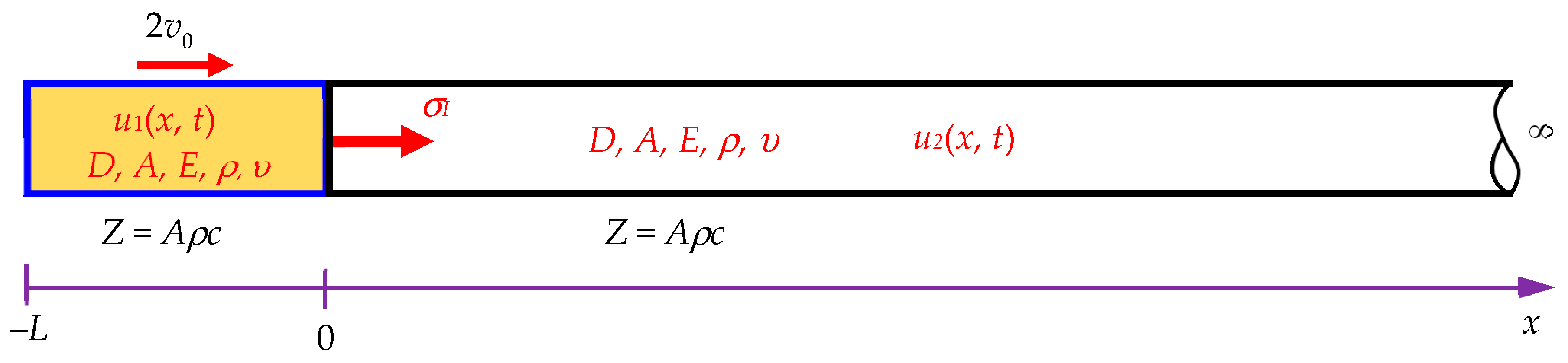
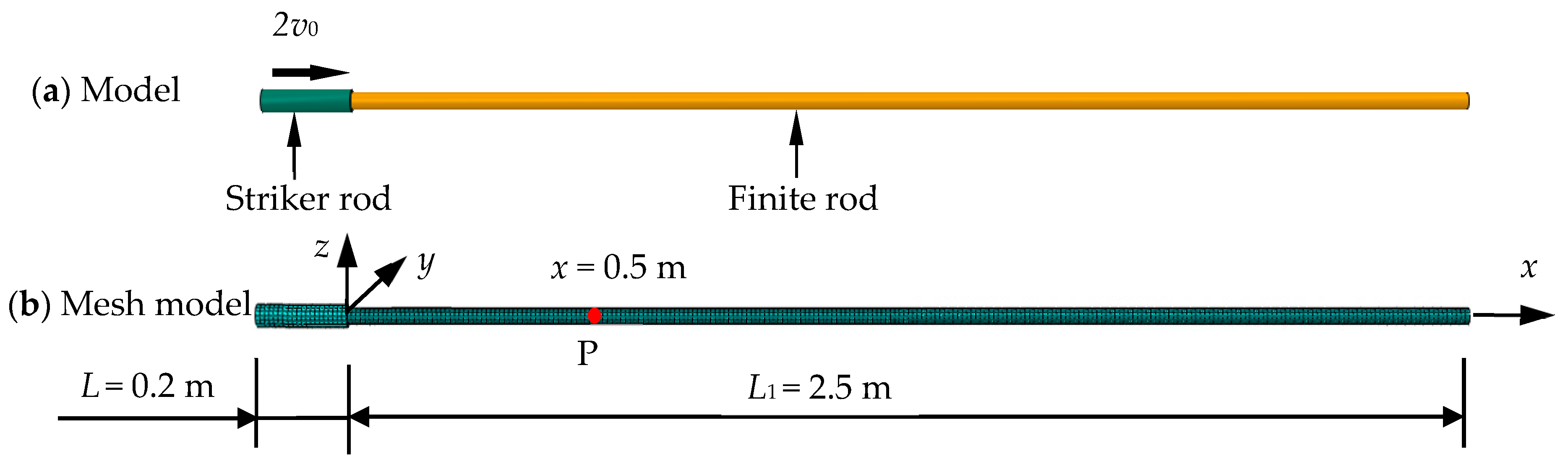
2. Materials and Methods
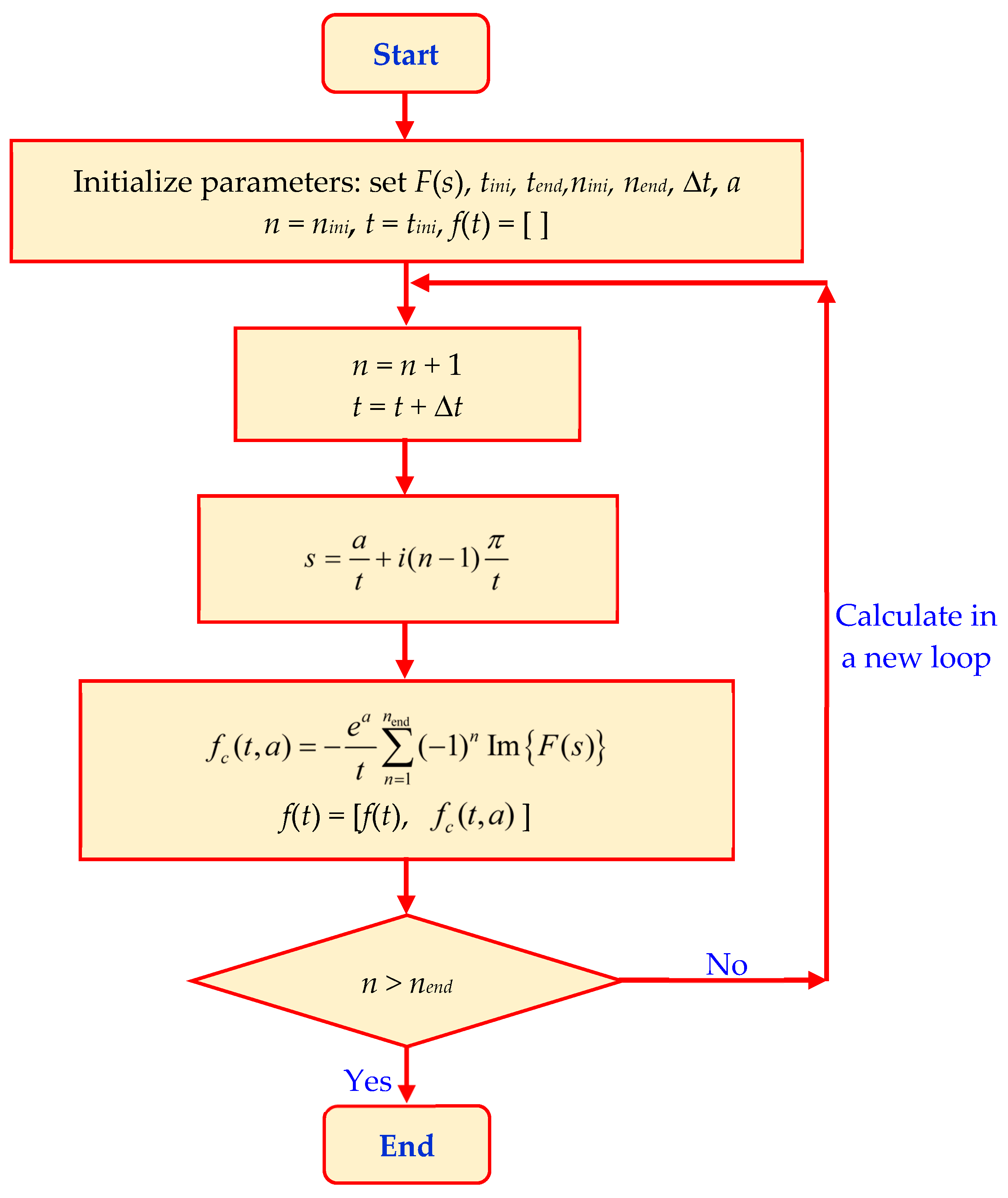
3. Inverse Laplace Transform
- F(s) is regular for Re{s} > 0.
- .
- F*(s) = F(s*), where the asterisk denotes the complex conjugate value.
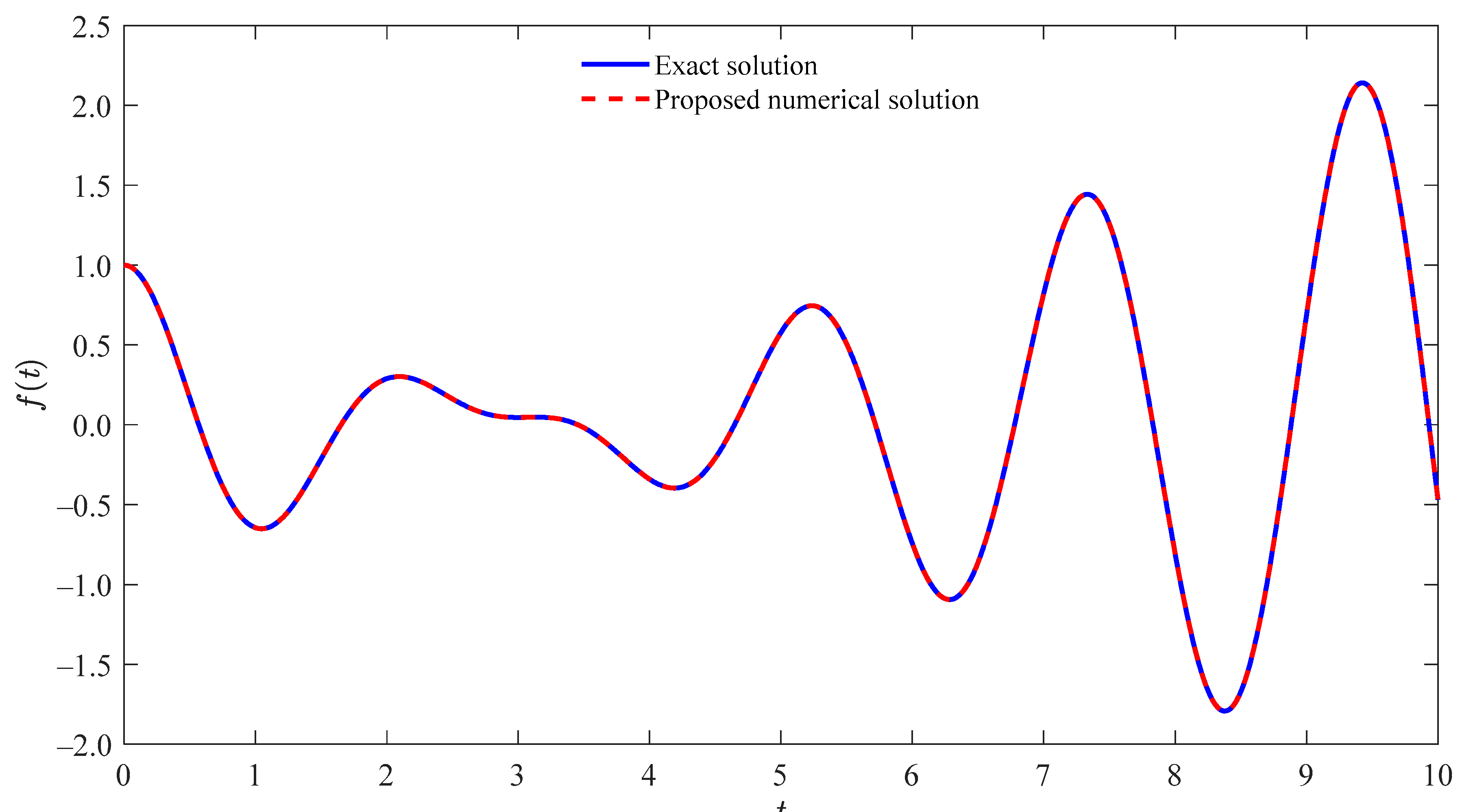
4. Validation of the Proposed Numerical Algorithm for the Inversion of Laplace Transformation
4.1. Exampe 1
4.2. Exampe 2
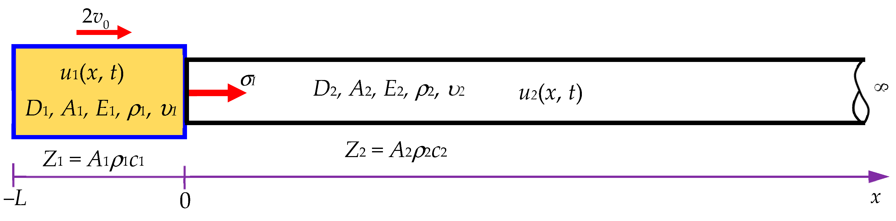
5. Investigation of Wave Propagation in a Rayleigh–Love Rod under the Collinear Impact of a Striker Rod with Different Impedances
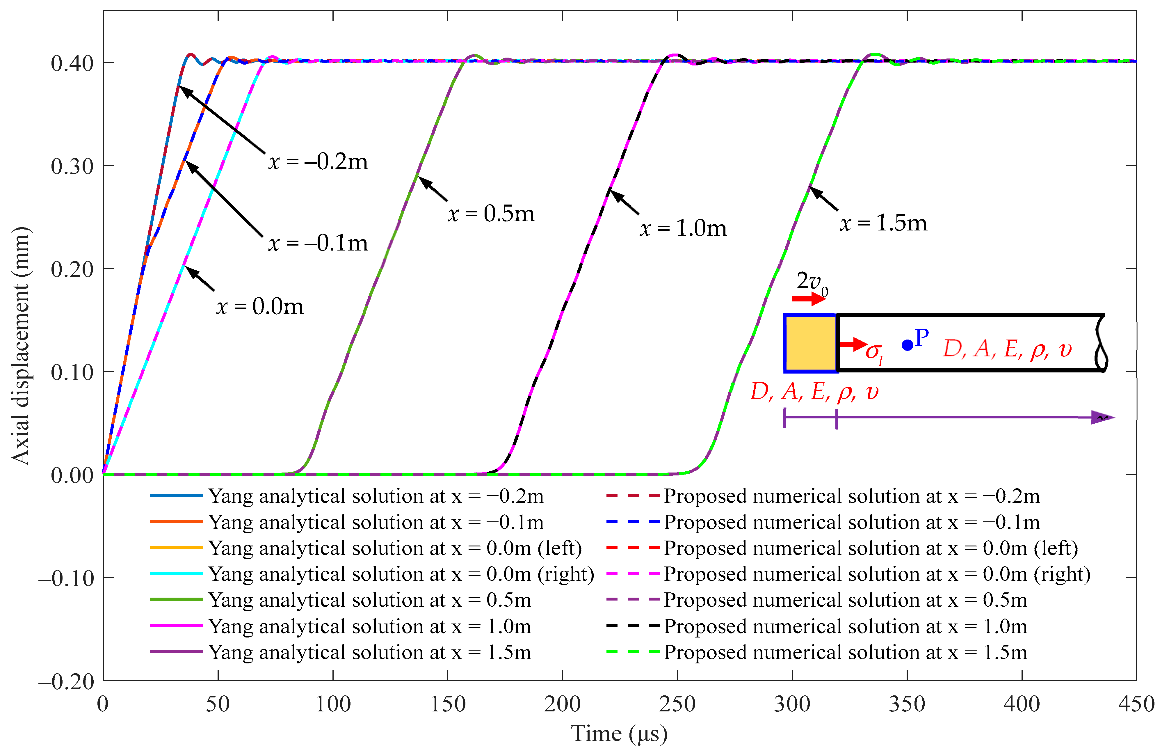
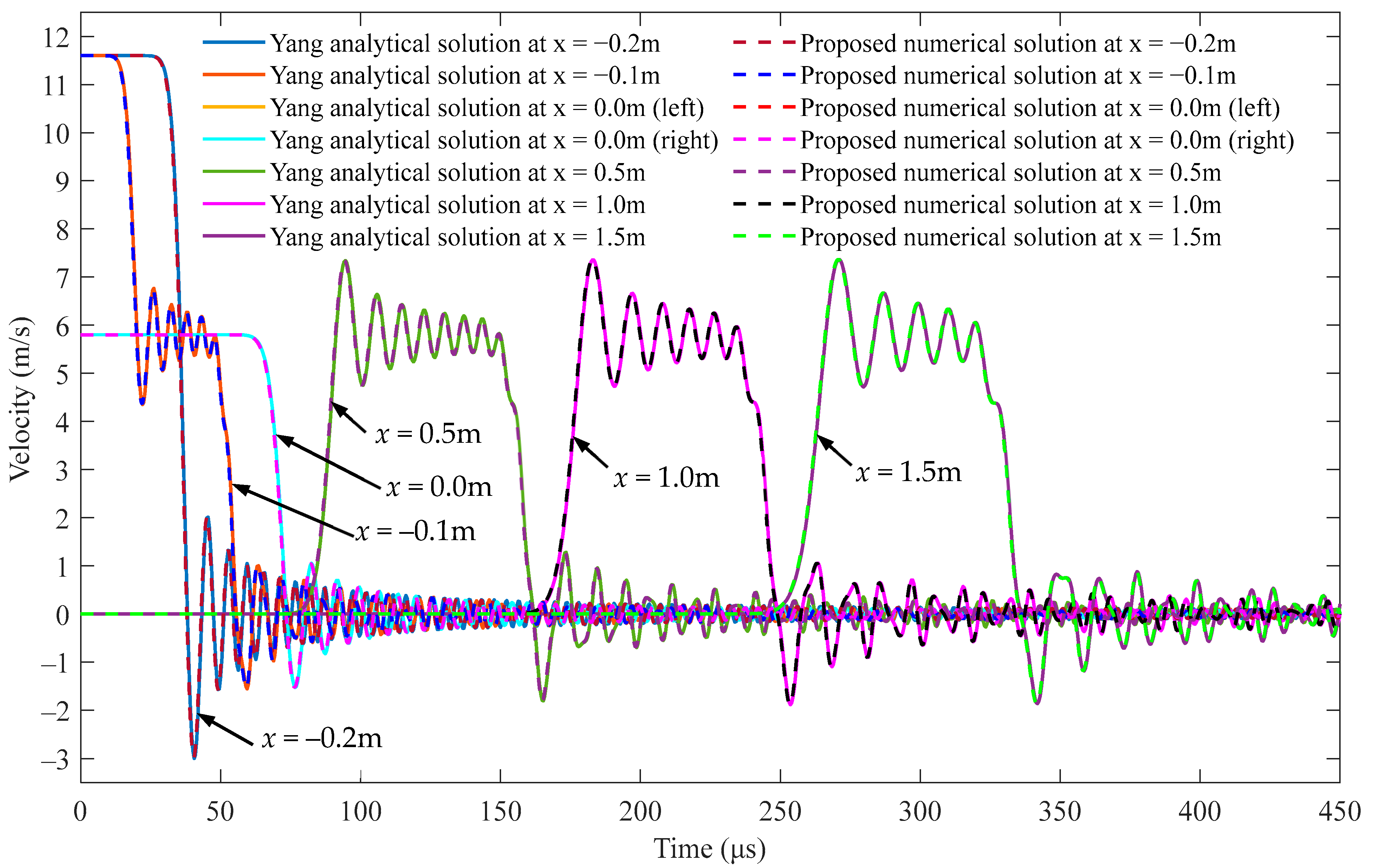
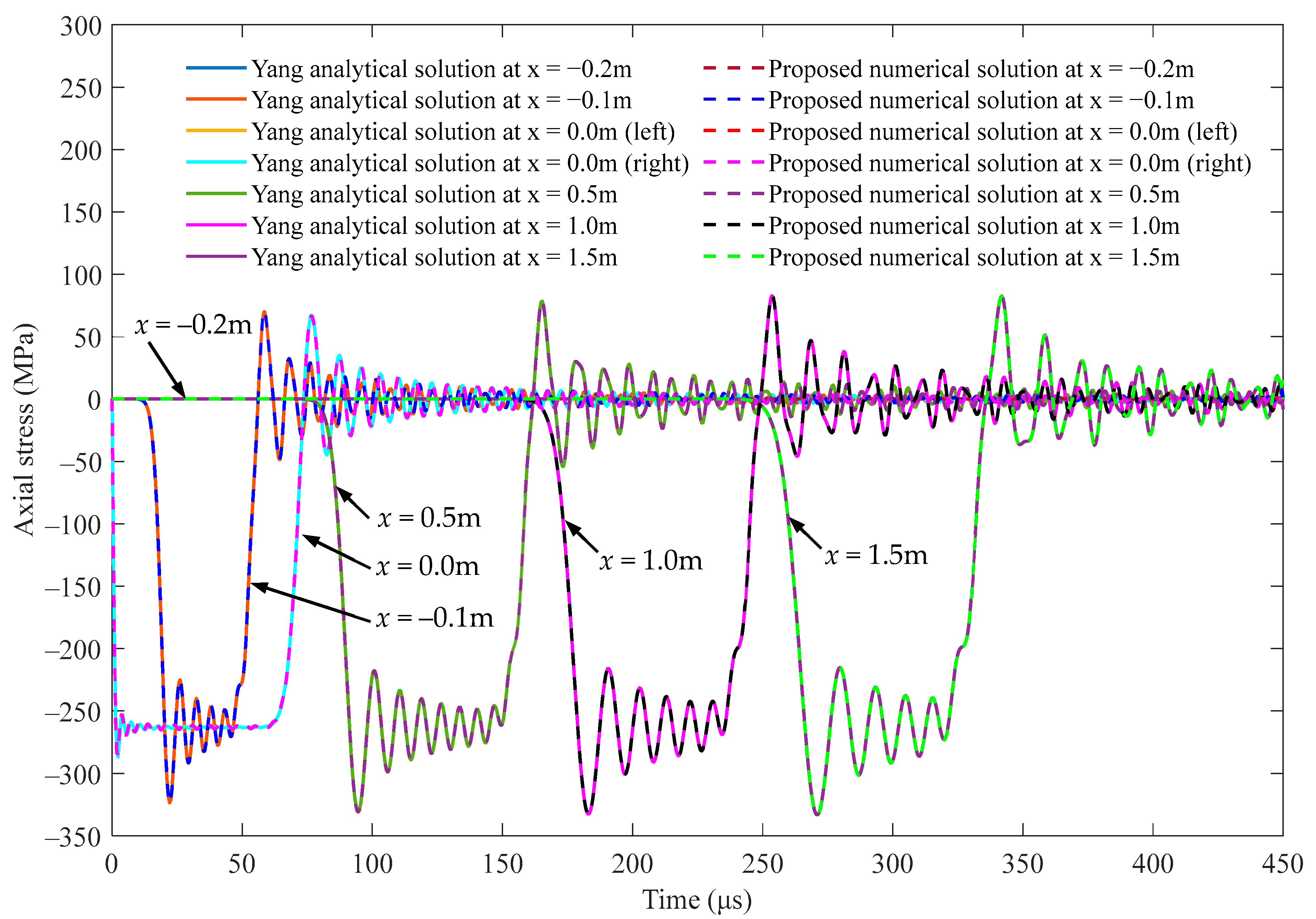
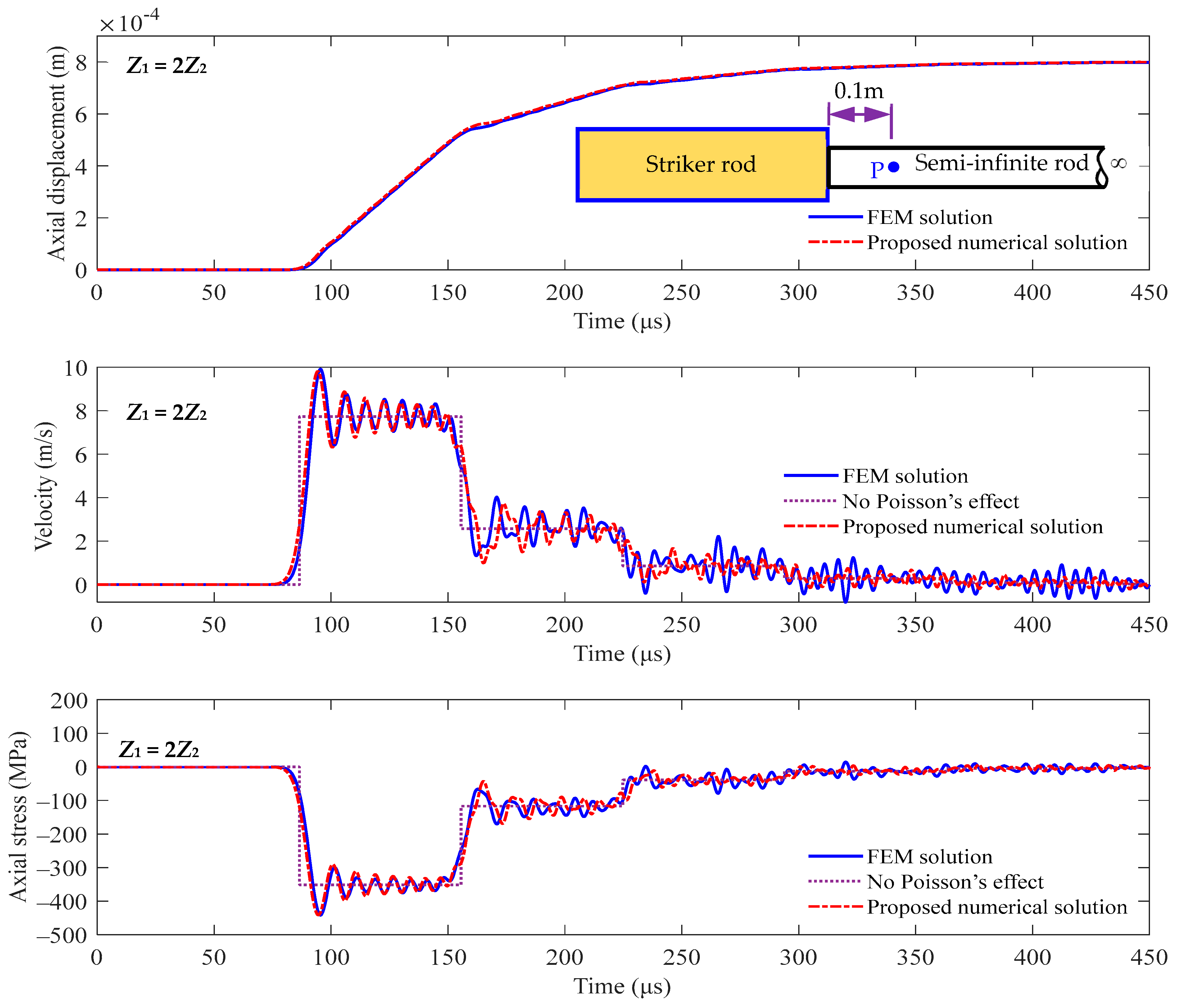
5.1. Investigation of Stress Wave Propagation in a Semi-Infinite Rod and a Striker Rod at the Interface x = 0 m
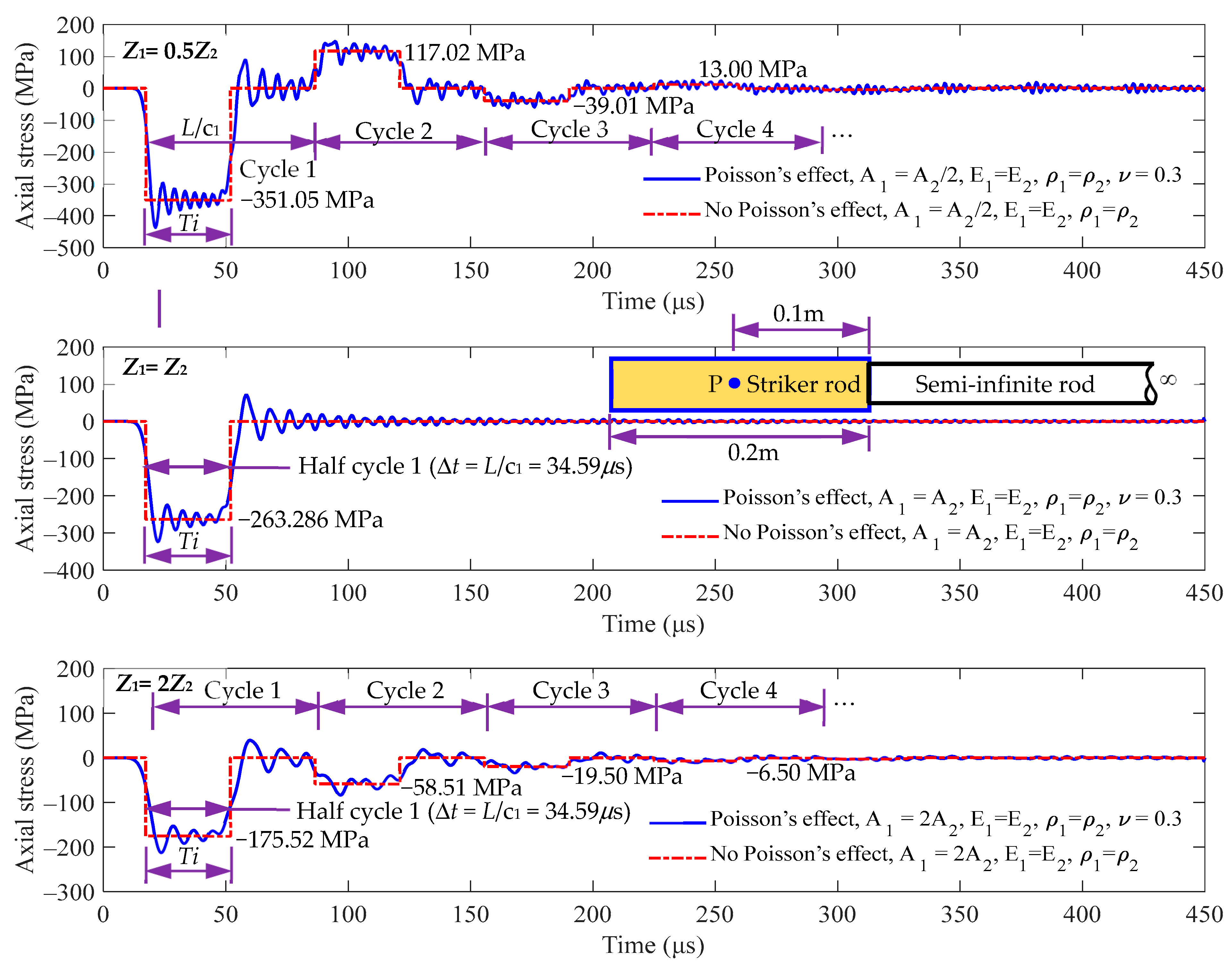
5.2. Investigation of Stress Wave Propagation in a Striker Rod at x = −0.1 m
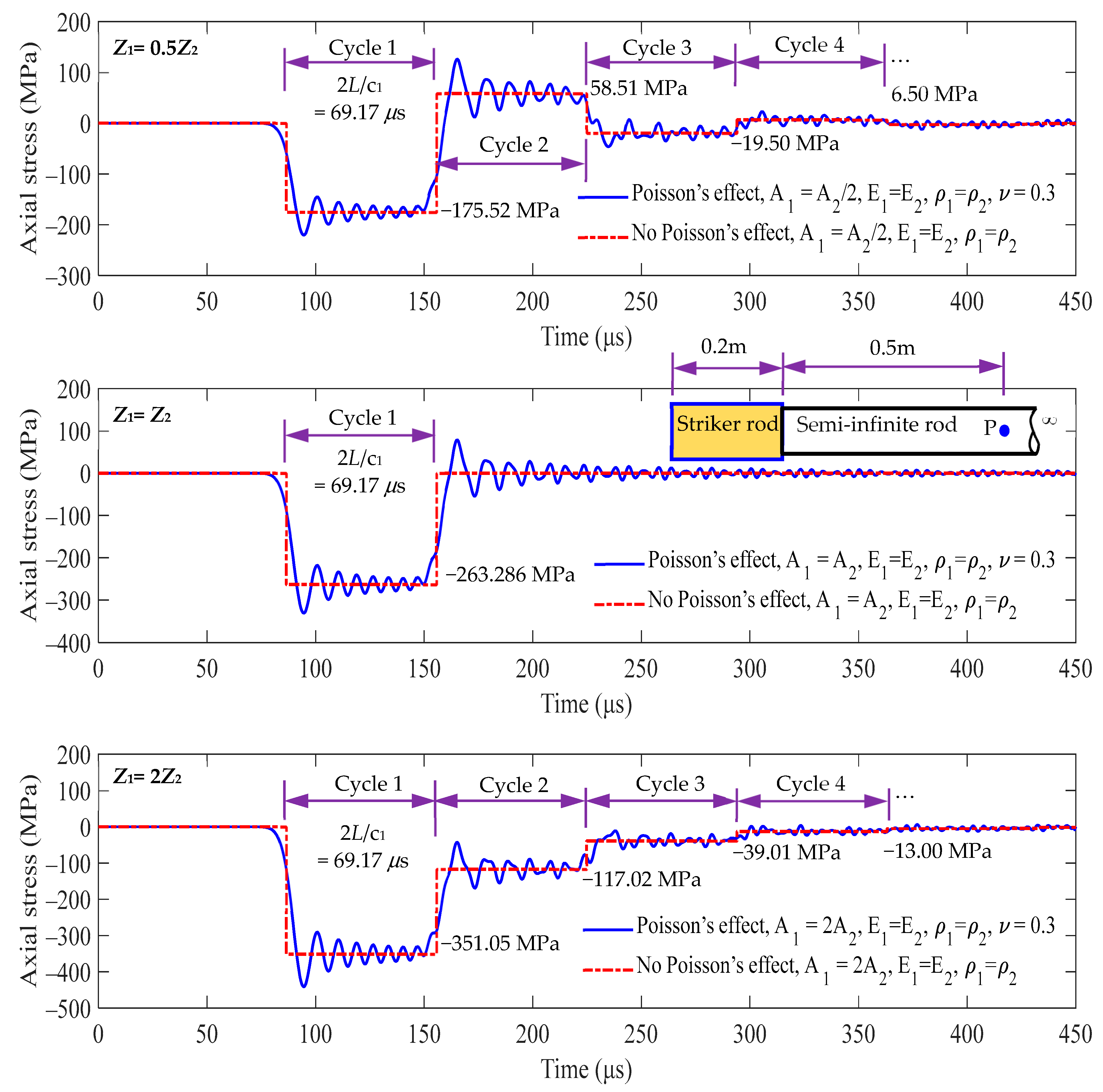
5.3. Investigation of Stress Wave Propagation in a Semi-Infinite Rod at x = 0.5 m
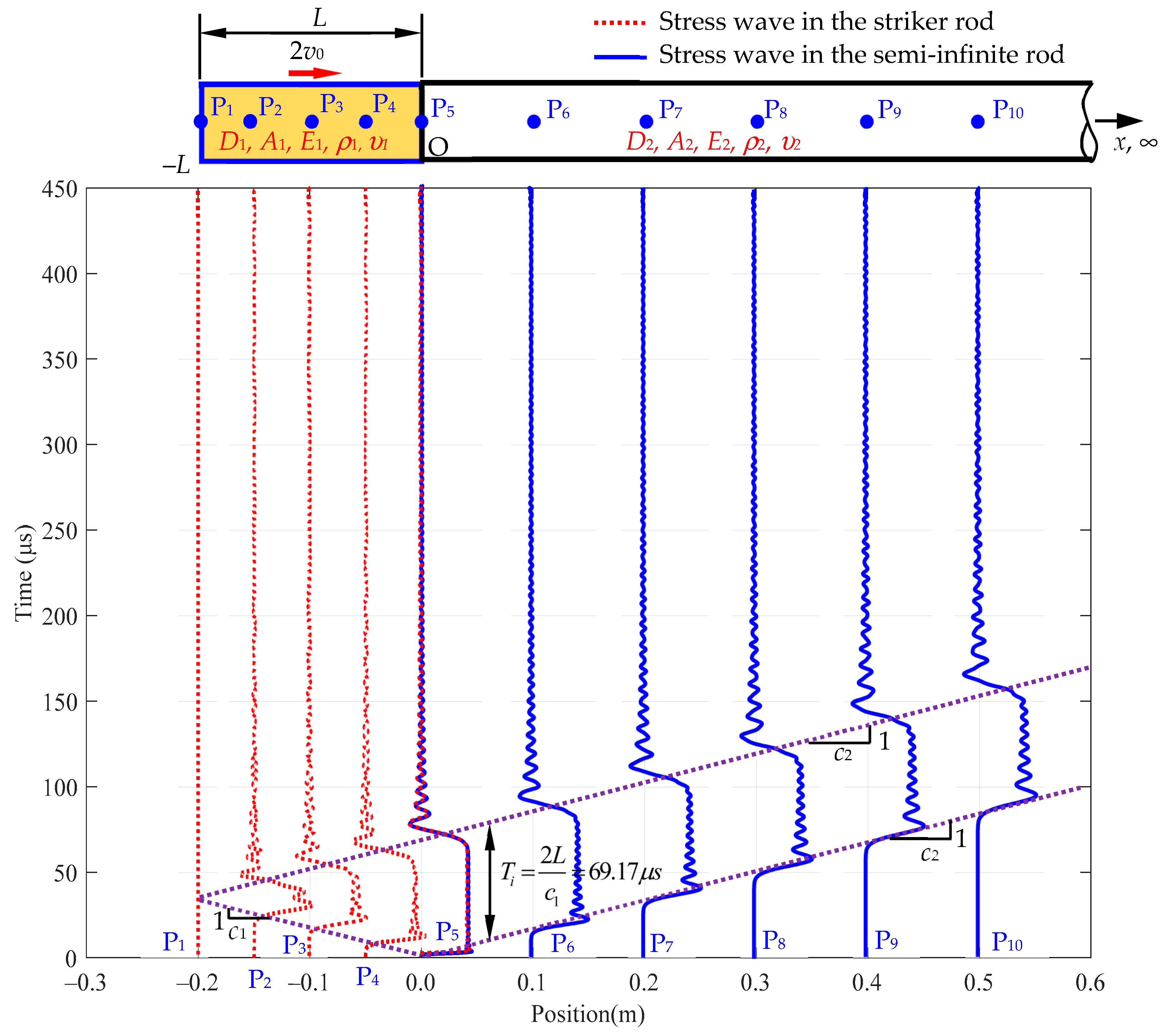
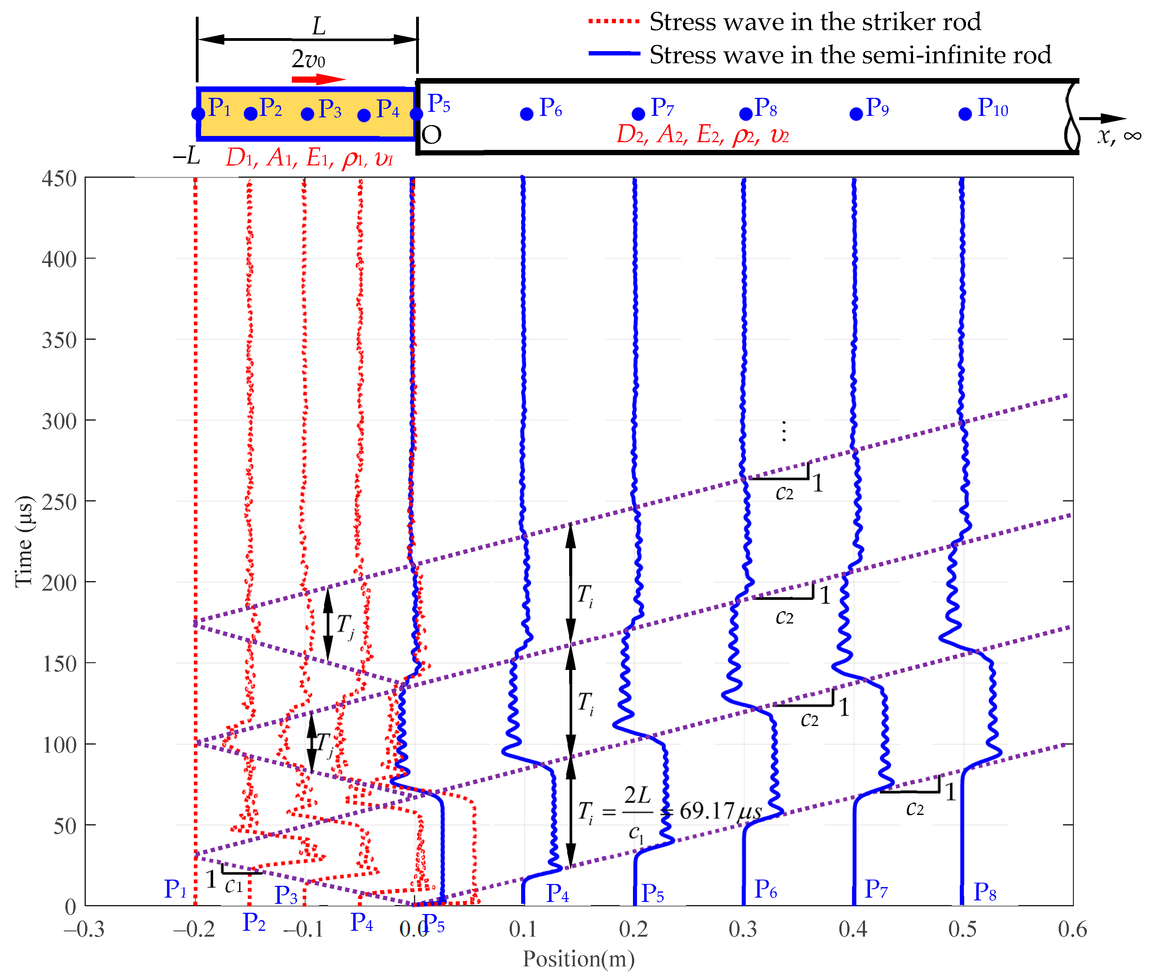
6. Travel Time History
7. Conclusions
Author Contributions
Funding
Institutional Review Board Statement
Informed Consent Statement
Data Availability Statement
Conflicts of Interest
Appendix A. Solution of Laplace Transform of Equations (11) and (12)
References
- Tesfamariam, S.; Martín-Pérez, B. Stress wave propagation for evaluation of reinforced concrete structures. In Non-Destructive Evaluation of Reinforced Concrete Structures; Woodhead Publishing: Sawston, UK, 2010; pp. 417–440. [Google Scholar]
- Sawangsuriya, A. Wave propagation methods for determining stiffness of geomaterials. In Wave Processes in Classical and New Solids; IntechOpen: London, UK, 2012. [Google Scholar]
- Ostachowicz, W.; Radzieński, M. Structural health monitoring by means of elastic wave propagation. J. Phys. Conf. Ser. 2012, 382, 012003. [Google Scholar] [CrossRef]
- Jamaludin, N.; Mba, D.; Bannister, R.H. Condition monitoring of slow-speed rolling element bearings using stress waves. Proc. Inst. Mech. Eng. Part E J. Process Mech. Eng. 2001, 215, 245–271. [Google Scholar] [CrossRef]
- Lee, B.C.; Staszewski, W.J. Modelling of Lamb waves for damage detection in metallic structures: Part II. Wave interactions with damage. Smart Mater. Struct. 2003, 12, 815. [Google Scholar] [CrossRef]
- Palacz, M.; Krawczuk, M. Analysis of longitudinal wave propagation in a cracked rod by the spectral element method. Comput. Struct. 2002, 80, 1809–1816. [Google Scholar] [CrossRef]
- Gaul, L.; Bischoff, S.; Sprenger, H.; Haag, T. Numerical and experimental investigation of wave propagation in rod-systems with cracks. Eng. Fract. Mech. 2010, 77, 3532–3540. [Google Scholar] [CrossRef]
- Wang, X.X.; Yu, T.; Yan, H.P.; Ding, J.F.; Li, Z.; Qin, Z.Y.; Chu, F.L. Application of stress wave theory for pyroshock isolation at spacecraft-rocket interface. Chin. J. Aeronaut. 2021, 34, 75–86. [Google Scholar] [CrossRef]
- Fang, X. A one-dimensional stress wave model for analytical design and optimization of oscillation-free force measurement in high-speed tensile test specimens. Int. J. Impact Eng. 2021, 149, 103770. [Google Scholar] [CrossRef]
- D’Alembert, J. Researches on the curve that a tense cord forms when set into vibration. Hist. Acad. R. Des Sci. BL Berl. 1747, 3, 214–249. [Google Scholar]
- Shin, H.; Kim, D. One-dimensional analyses of striker impact on bar with different general impedance. Proc. Inst. Mech. Eng. Part C J. Mech. Eng. Sci. 2020, 234, 589–608. [Google Scholar] [CrossRef]
- Love, A.E.H. A Treatise on the Mathematical Theory of Elasticity; Dover Publications: New York, NY, USA, 1944. [Google Scholar]
- Yang, H.; Li, Y.; Zhou, F. Propagation of stress pulses in a Rayleigh-Love elastic rod. Int. J. Impact Eng. 2021, 153, 103854. [Google Scholar] [CrossRef]
- Yang, H.; Li, Y.; Zhou, F. Stress waves generated in a Rayleigh–Love rod due to impacts. Int. J. Impact Eng. 2022, 159, 104027. [Google Scholar] [CrossRef]
- Valsa, J.; Brančik, L. Approximate formulae for numerical inversion of Laplace transforms. Int. J. Numer. Model. Electron. Netw. Devices Fields 1998, 11, 153–166. [Google Scholar] [CrossRef]
- Wang, C.Y.; Thang, N.N.; Wang, H. Stress Wave Propagation in a Rayleigh–Love Rod with Sudden Cross-Sectional Area Variations Impacted by a Striker Rod. Sensors 2024, 24, 4230. [Google Scholar] [CrossRef] [PubMed]
- Carrier, G.F.; Krook, M.; Pearson, C.E. Functions of a Complex Variable: Theory and Technique; McGraw Hill: New York, NY, USA, 1966. [Google Scholar]
- Juraj. Numerical Inversion of Laplace Transforms in Matlab. MATLAB Central File Exchange. 2024. Available online: https://www.mathworks.com/matlabcentral/fileexchange/32824-numerical-inversion-of-laplace-transforms-in-matlab (accessed on 24 January 2024).
- Schiff, J.L. The Laplace Transform: Theory and Applications; Springer: Berlin/Heidelberg, Germany, 1999. [Google Scholar]
- Dassault Systèmes. Abaqus Analysis User’s Guide, Volume II: Analysis; Dassault Systèmes: Providence, RI, USA, 2016. [Google Scholar]


| Parameters | Striker Rod | Semi-Infinite Rod |
|---|---|---|
| Diameter, D (mm) | 30 (A1/A2 = 1) | 30 |
| Young’s modulus, E (GPa) | 195 (E1/E2 = 1) | 195 |
| Mass density, ρ (kg/m3) | 7850 (ρ1/ρ2 = 1) | 7850 |
| Poisson’s ratio, υ | 0.3 | 0.3 |
| Rod length, L (m) | 0.2 | ∞ |
| Initial velocity, 2v0 (m/s) | 11.6 | 0 |
| Wave speed, c (m/s) | 5782.69 | 5782.69 |
| Impedance, Z = Aρc (kg/s) | 32,087.204 | 32,087.204 |
| Parameters | Striker Rod | Semi-Infinite Rod |
|---|---|---|
| Diameter, D (mm) | 21.213 (A1/A2 = 0.5) 30 (A1/A2 = 1) 42.426 (A1/A2 = 2) | 30 |
| Young’s modulus, E (GPa) | 195 | 195 |
| Mass density, ρ (kg/m3) | 7850 | 7850 |
| Poisson’s ratio, υ | 0.3 | 0.3 |
| Yield stress, σ0 (MPa) | 1275 | 1275 |
| Cycle | Z1 = 0.5Z2 | Z1 = Z2 | Z1 = 2Z2 | ||||||
|---|---|---|---|---|---|---|---|---|---|
| Time (μs) | σ1 (MPa) | σ2 (MPa) | Time (μs) | σ1 (MPa) | σ2 (MPa) | Time (μs) | σ1 (MPa) | σ2 (MPa) | |
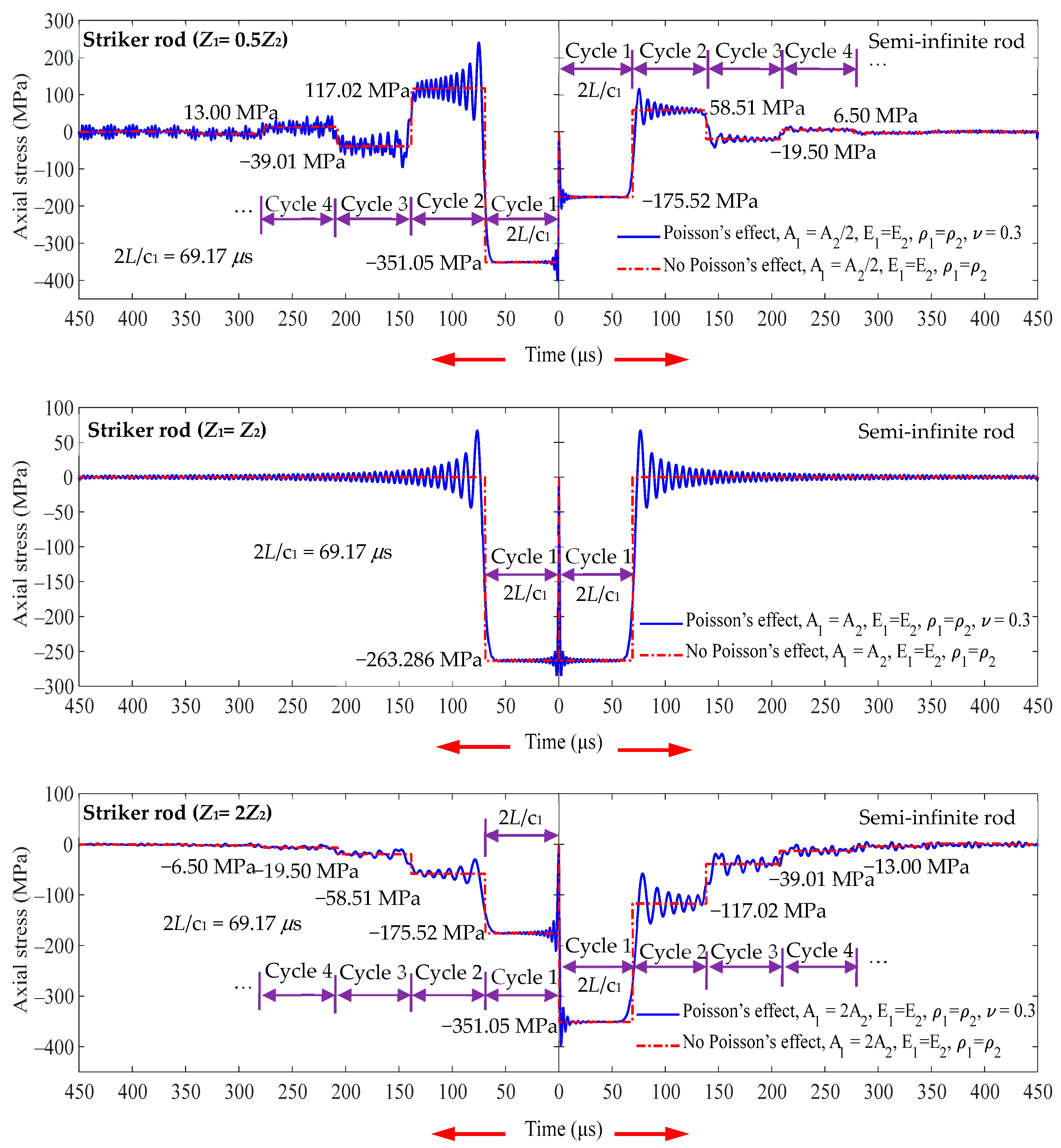
| 1 | 0~69.17 | −351.05 | −175.52 | 0~69.17 | −263.286 | −263.286 | 0~69.17 | −175.52 | −351.05 |
| 2 | 69.17~138.34 | 117.02 | 58.508 | 69.17~138.34 | 0 | 0 | 69.17~138.34 | −58.51 | −117.02 |
| 3 | 138.34~207.52 | −39.01 | −19.50 | 138.34~207.52 | 0 | 0 | 138.34~207.52 | −19.50 | −39.01 |
| 4 | 207.52~276.69 | 13.00 | 6.50 | 207.52~276.69 | 0 | 0 | 207.52~276.69 | −6.501 | −13.00 |
| 5 | 276.69~345.86 | −4.33 | −2.17 | 276.69~345.86 | 0 | 0 | 276.69~345.86 | −2.17 | −4.33 |
| Cycle | Z1 = 0.5Z2 | Z1 = Z2 | Z1 = 2Z2 | ||||
|---|---|---|---|---|---|---|---|
| Time (μs) | σ1 (MPa) | Time (μs) | σ1 (MPa) | Time (μs) | σ1 (MPa) | ||
| 1 | 1/2 | 17.29~51.88 | −351.05 | 17.29~51.88 | −263.286 | 17.29~51.88 | −175.52 |
| 1/2 | 51.88~86.46 | 0 | 51.88~86.46 | 0 | 51.88~86.46 | 0 | |
| 2 | 1/2 | 86.46~121.05 | 117.02 | 86.46~121.05 | 0 | 86.46~121.05 | −58.51 |
| 1/2 | 121.05~155.64 | 0 | 121.05~155.64 | 0 | 121.05~155.64 | 0 | |
| 3 | 1/2 | 155.64~190.22 | −39.01 | 155.64~190.22 | 0 | 155.64~190.22 | −19.5 |
| 1/2 | 190.22~224.81 | 0 | 190.22~224.81 | 0 | 190.22~224.81 | 0 | |
| 4 | 1/2 | 224.81~259.39 | 13.00 | 224.81~259.39 | 0 | 224.81~259.39 | −6.50 |
| 1/2 | 259.39~293.98 | 0 | 259.39~293.98 | 0 | 259.39~293.98 | 0 | |
| 5 | 1/2 | 293.98~328.57 | −4.33 | 293.98~328.57 | 0 | 293.98~328.57 | −2.17 |
| 1/2 | 328.57~363.15 | 0 | 328.57~363.15 | 0 | 328.57~363.15 | 0 | |
| Cycle | Z1 = 0.5Z2 | Z1 = Z2 | Z1 = 2Z2 | |||
|---|---|---|---|---|---|---|
| Time (μs) | σ2 (MPa) | Time (μs) | σ2 (MPa) | Time (μs) | σ2 (MPa) | |
| 1 | 86.46~155.64 | −175.52 | 86.46~155.64 | −263.286 | 86.46~155.64 | −351.05 |
| 2 | 155.64~224.81 | 58.51 | 155.64~224.81 | 0 | 155.64~224.81 | −117.02 |
| 3 | 224.81~293.98 | −19.50 | 224.81~293.98 | 0 | 224.81~293.98 | −39.01 |
| 4 | 293.98~363.15 | 6.50 | 293.98~363.15 | 0 | 293.98~363.15 | −13.00 |
| 5 | 363.15~432.32 | −2.167 | 363.15~432.32 | 0 | 363.15~432.32 | −4.33 |
Disclaimer/Publisher’s Note: The statements, opinions and data contained in all publications are solely those of the individual author(s) and contributor(s) and not of MDPI and/or the editor(s). MDPI and/or the editor(s) disclaim responsibility for any injury to people or property resulting from any ideas, methods, instructions or products referred to in the content. |
© 2024 by the authors. Licensee MDPI, Basel, Switzerland. This article is an open access article distributed under the terms and conditions of the Creative Commons Attribution (CC BY) license (https://creativecommons.org/licenses/by/4.0/).
Share and Cite
Thang, N.N.; Wang, C.-Y. Stress Wave Propagation in a Semi-Infinite Rayleigh–Love Rod under the Collinear Impact of a Striker Rod with Different General Impedances. Appl. Sci. 2024, 14, 6523. https://doi.org/10.3390/app14156523
Thang NN, Wang C-Y. Stress Wave Propagation in a Semi-Infinite Rayleigh–Love Rod under the Collinear Impact of a Striker Rod with Different General Impedances. Applied Sciences. 2024; 14(15):6523. https://doi.org/10.3390/app14156523
Chicago/Turabian StyleThang, Nguyen Ngoc, and Chung-Yue Wang. 2024. "Stress Wave Propagation in a Semi-Infinite Rayleigh–Love Rod under the Collinear Impact of a Striker Rod with Different General Impedances" Applied Sciences 14, no. 15: 6523. https://doi.org/10.3390/app14156523