Analytical Investigation of Vertical Force Control in In-Wheel Motors for Enhanced Ride Comfort

Abstract

This study explores the effectiveness of vertical force control in in-wheel motors (IWMs) to enhance ride comfort in electric vehicles (EVs). A dynamic vehicle model and a proportional ride-blending controller were used to reduce vertical vibrations of the sprung mass. By converting the state-space model into a transfer function, the system’s frequency response was evaluated using road profiles generated according to ISO 8608 standards and converted into Power Spectral Density (PSD) inputs. The frequency-weighted acceleration ($a_w$) was calculated based on ISO 2631 standards to measure ride comfort improvements. The results showed that increasing the proportional gain ($K_p$) effectively reduced the frequency-weighted acceleration and the RMS of the vertical acceleration of the sprung mass. However, the proportional gain could not be increased indefinitely due to the torque limitations of the IWMs. Optimal proportional gains for various road profiles demonstrated significant improvements in ride comfort. This study concludes that advanced suspension technologies, including the proportional ride-blending controller, can effectively mitigate the challenges of increased unsprung mass in IWM vehicles, thereby enhancing ride quality and vehicle dynamics.

1. Introduction

The rapid rise of electric vehicles (EVs) is transforming the automotive industry. Central to this transformation is the use of in-wheel motors (IWMs), a technology first proposed in 1900. Today, with the growing market potential of EVs, IWMs have emerged as a promising approach to revolutionize vehicle design and performance [1,2]. Relocating the motor to the wheel brings numerous advantages. It reduces the overall vehicle weight, thereby increasing driving range, reducing running costs, and minimizing the frequency of battery charging. Additionally, IWMs improve handling due to precise torque control on each wheel, resulting in enhanced stability, traction control, and shorter stopping distances. This technology also offers more efficient production and flexible vehicle design, making it economically attractive for manufacturers.

However, integrating IWMs into vehicle wheels increases unsprung mass, adversely affecting ride comfort and handling, especially at high speeds [3]. Each IWM adds 30–52 kg per wheel, significantly boosting unsprung mass and reducing the body-to-wheel mass ratio [4]. This imbalance compromises ride smoothness, particularly at high frequencies where dynamic load changes are more pronounced. The increased unsprung mass causes the wheels to react more intensely to road irregularities, resulting in greater vertical vibrations. When the dynamic load and dead load are equal but opposite, the vertical load drops to zero, causing the wheel to lose contact with the road. This loss of adhesion can make driving dangerous during high-speed driving or sudden maneuvers [3]. Furthermore, this situation stresses suspension components, increasing wear and potential damage. Maintaining tire contact with the road is crucial for safety and performance, as any loss of contact reduces stability and control [3,5].

To address these challenges, vehicle suspension systems play a critical role in transmitting forces between the wheels and the vehicle frame, reducing shocks from rough roads, and ensuring driving smoothness and stability. Extensive research has focused on developing both active and passive suspension systems to enhance vehicle performance. One common solution involves applying passive suspensions with springs and dampers between the IWM and the wheel to improve comfort [1,6,7,8,9,10,11,12,13,14,15]. However, these systems often fail to address the relative vertical displacement or vibration of the IWM, necessitating more advanced solutions.

These challenges require advanced suspension systems, such as semi-active or active systems equipped with magneto-rheological (MR) [7,9,16], hydraulic (HA) [17], or electromagnetic (EMA) absorbers [18]. Numerous control techniques have been developed to enhance vehicle ride and handling, ranging from comfort-oriented sky-hook to handling-oriented ground-hook and multi-objective linear optimal control techniques [6]. Despite these advancements, traditional suspension systems cannot fully eliminate vibrations across all frequency ranges, necessitating a compromise between ride comfort and handling performance. This compromise is further exacerbated in IWM vehicles due to the increased unsprung mass, highlighting the need for more sophisticated suspension technologies to maintain optimal ride quality and vehicle control.

Configurations using MR dampers showed low efficiency [9], with unchanged trade-offs between low- and high-frequency responses. Dynamic dampers like tuned mass dampers (TMDs) can partially reduce this issue. Ref. [8] reported a 31.2% improvement in ride comfort and a 2.2% increase in road holding. Ref. [19] introduced a compact electromagnetic TMD, achieving a 21.7% increase in comfort and a 5.7% improvement in handling. Refs. [5,10,13] demonstrated a two-stage optimization control reducing body acceleration by 11.34% and impulse force on the IWM by 88.57%. Despite these advances, implementation remains challenging due to limited wheel space and system robustness.

Then, to address these challenges, researchers have explored advanced control strategies for active suspension systems in in-wheel motor-driven electric vehicles (IWMD-EVs). One notable approach is the mixed $H_2$/$H_{\infty }$-based robust guaranteed cost control system, which integrates dynamic vibration absorbers into the active suspension model to significantly improve ride comfort and handling stability. Ref. [20] demonstrated through simulations that this controller can outperform traditional passive suspensions and standalone $H_{\infty }$ controllers, offering a marked improvement in overall vehicle dynamics.

Additionally, decentralized dynamic event-triggered communication mechanisms have been developed to enhance control efficiency in IWMD-EVs. Ref. [21] has proposed a decentralized dynamic event-triggered control approach that not only improves ride comfort but also reduces the communication load. Adaptive control strategies, such as sliding mode control and fuzzy logic systems, also have shown significant effectiveness in addressing the nonlinearity and time-varying dynamics inherent in active suspensions. Refs. [14,22] have developed robust adaptive controllers that ensure consistent tire–road contact and vehicle stability under varying load conditions and road profiles.

Furthermore, regenerative active suspension systems have been explored to harness residual energy from suspension movements. Ref. [23] demonstrated that such systems can improve energy efficiency while maintaining or enhancing ride comfort and handling. Model predictive control (MPC) has emerged as a promising approach for real-time optimization of suspension performance. Ref. [24] showed that MPC can effectively balance ride comfort and handling by predicting future states and optimizing control inputs accordingly. Despite these advancements, practical implementation challenges persist, particularly due to limited wheel space and the need for robust control systems [25,26,27]. Further research and development are required to fully realize the potential of these advanced suspension technologies in IWMD-EVs.

One promising solution to the suspension issue is the ride-blending control method. Simulations by Ref. [3] showed that this technique effectively reduces the pitch response of the vehicle body by leveraging the vertical component of the driving force, all while keeping the tire dynamic force within safe limits. Ride-blending control works by integrating vehicle dynamics through electronic brake distribution and active suspension systems, coordinated in a decentralized manner [28]. Essentially, when one system is active, the other minimizes its force, ensuring a balanced and efficient performance. This method offers a more refined approach to handling the challenges posed by increased unsprung mass in IWM vehicles.

Ref. [1] demonstrates the development of ride-blending control, a strategy that utilizes the vertical component of IWM driving force to enhance ride comfort and handling. Simulation tests on a vehicle model with coupled dynamics showed a 31.8% improvement in ride comfort without impacting tire load or longitudinal dynamics. The method also confirmed stable lateral dynamics.

It seems that ride-blending control has significant potential to improve ride comfort, as demonstrated by various studies [1,3,28]. However, most of these studies present results in the time domain and in terms of sprung mass acceleration. This research extends the findings of Ref. [1] and aims to develop a proportional ride-blending controller for a vehicle and analyze the results in the frequency domain to better understand how well ride-blending control can improve suspension performance. Additionally, frequency-weighted acceleration will be calculated to compare ride comfort. The contribution of this research lies in the investigation of proportional ride-blending control in the frequency domain and its impact on enhancing ride comfort for EVs with IWMs.

2. Dynamics Models and Methods

To investigate how vertical force control in IWMs can enhance ride comfort, a dynamic vehicle model in state-space form is developed. A proportional ride-blending controller is then implemented, transforming the model into a multiple-input single-output (MISO) system. The state-space model is converted into a transfer function to analyze the system’s frequency response. To evaluate ride comfort, road profiles are generated according to ISO 8608 standards [29] and converted into Power Spectral Density (PSD) inputs for the vehicle model. Both the open-loop and closed-loop systems of the vehicle are simulated, and the results are collected. Finally, frequency-weighted acceleration (${\mathit{a}}_{\mathit{w}}$) is calculated according to ISO 2631 standards [30] to assess ride comfort improvements.

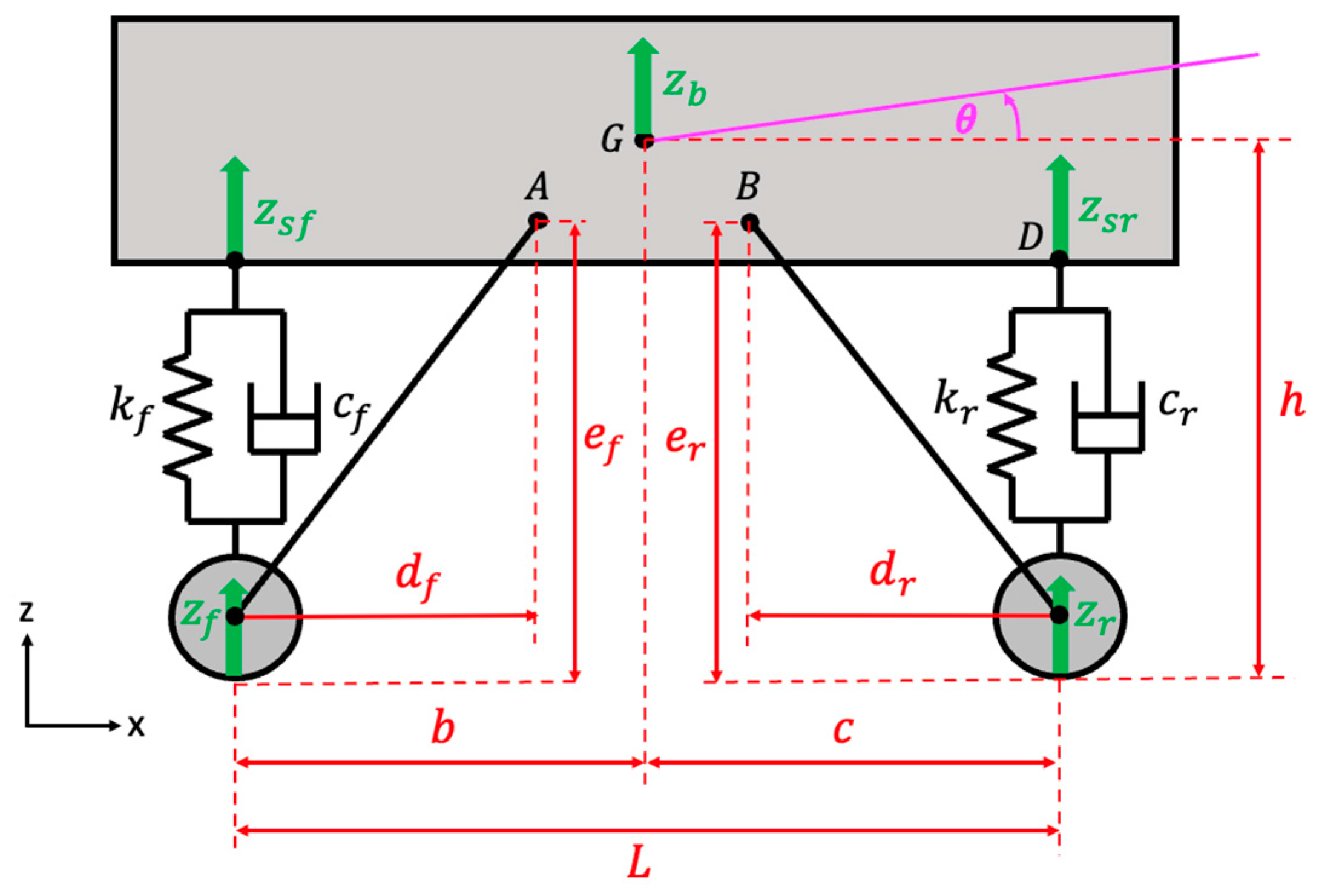
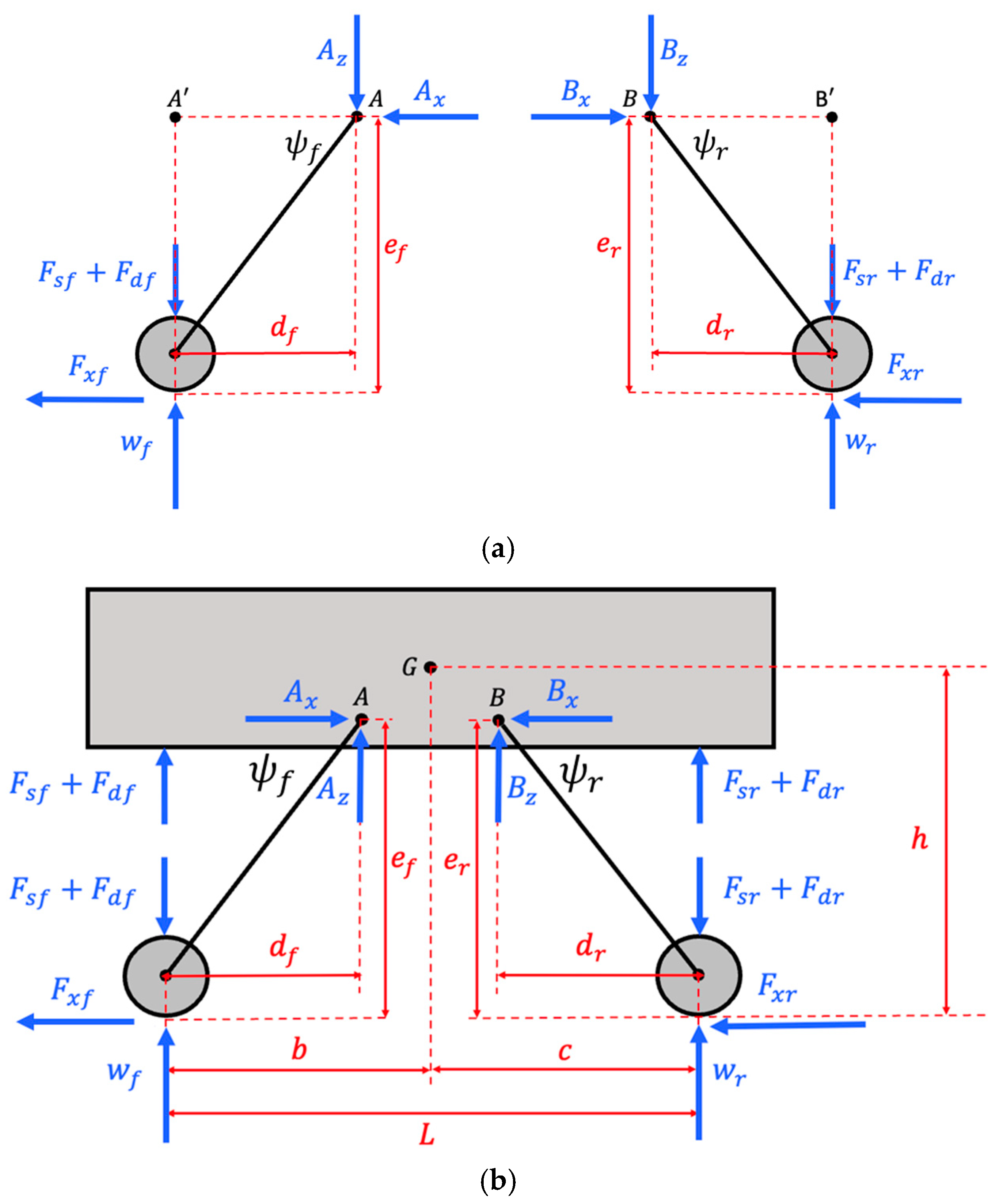
2.1. Vehicle Dynamics Model

The ride-blending controller leverages the construction constraints of typical suspensions, which have rotational centers for both roll and pitch movements in the longitudinal direction. This rotational movement allows the suspension to transfer some of the tire’s driving force into a vertical direction. The vertical component of this driving force can then be utilized to control the dynamics of the vehicle’s sprung mass. To examine the impact of controlling the vertical component of the driving force on the vehicle’s dynamics, a half-vehicle model is introduced. This model includes longitudinal and vertical dynamics, as illustrated in Figure 1.

Based on Figure 1, point G represents the center of gravity of the sprung mass, while points A and B are the positions of the shafts connecting the wheels to the sprung mass. The forces from the wheels can be transmitted to the sprung mass through these points. Additionally, the sprung mass is supported by the suspension system at both the front and rear wheels. For simplicity, the wheels are assumed to be rigid bodies, meaning their positions, $z_f$ and $z_r$, equal the elevation of the road profile.

The free body diagram in Figure 2a shows that

$$A_x=-F_{xf}$$

(1)

$$B_x=F_{xr}$$

(2)

where $F_{xf}$ is additional front longitudinal drive force and $F_{xr}$ is additional rear longitudinal drive force.

Also, based on Figure 2a, the vertical forces in terms of the tire’s driving forces can be presented as follows [1,3,31,32]:

$$A_z=-F_{xf}tan{\psi }_f=-F_{xf}{\displaystyle \frac{e_f}{d_f}}$$

(3)

$$B_z=F_{xr}tan{\psi }_r=F_{xr}{\displaystyle \frac{e_r}{d_r}}$$

(4)

where $A_z$ is front vertical force from the front longitudinal drive force, $B_z$ is rear vertical force from the rear longitudinal drive force, $e_f$ is the vertical distance from the ground to point A, $e_r$ is the vertical distance from the ground to point B, $d_f$ is the horizontal distance from the front wheel to point A, and $d_r$ is the horizontal distance from the rear wheel to point B.

Based on Figure 2b, the vehicle dynamics of the sprung mass are

$$m_s{\ddot{z}}_b=F_{sf}+F_{sr}+F_{df}+F_{dr}+A_z+B_z$$

(5)

$$\begin{array}{c}{I}_z\ddot{\theta }=(-b\left(F_{sf}+F_{df}\right)+c\left(F_{sr}+F_{dr}\right)\\ +\left(h-e_f\right)A_x-\left(b-d_f\right)A_z-\left(h-e_r\right)B_x+(c-d_r)B_z)\end{array}$$

(6)

where $z_b$ is the vertical displacement of sprung mass, $\theta$ is the pitch angel of sprung mass, $m_s$ is the sprung mass, $I_z$ is the pitch inertia of the sprung mass, $F_{sf}$ and $F_{sr}$ are front and rear spring forces from the suspension, $F_{df}$ and $F_{dr}$ are front and rear damping forces from the suspension, and $b$, $c$, $d_f$, $d_r$, and $h$ are the distance according to Figure 2b.

The suspension forces are defined as follows:

$$F_{sf}=k_f\left(z_f-z_{sf}\right)=k_f\left(z_f-(z_b-b\theta )\right)$$

(7)

$$F_{sr}= k_r\left(z_r-z_{sr}\right)= k_r(z_r-(z_b+c\theta \left)\right)$$

(8)

$$F_{df}= c_f\left({\dot{z}}_f-{\dot{z}}_{sf}\right)= c_f({\dot{z}}_f-({\dot{z}}_b-b\dot{\theta }\left)\right)$$

(9)

$$F_{dr}= c_r\left({\dot{z}}_r-{\dot{z}}_{sr}\right)= c_r({\dot{z}}_r-({\dot{z}}_b+c\dot{\theta }\left)\right)$$

(10)

where $k_f$ and $k_r$ are the front and rear spring stiffness, and $c_f$ and $c_r$ are the front and rear damping coefficients.

For the case where there is no additional front and rear longitudinal drive force, $F_{xf}=F_{xr}=0$, there is no vertical component of the driving force; $A_z=B_z=0$. This system is an uncontrolled or open-loop system. The dynamics model of the system is determined as follows: substitute Equations (1)–(4) and (7)–(10) into Equations (5) and (6), and then the vehicle dynamics of the sprung mass are defined by

$$\begin{array}{c}{\ddot{z}}_b=-{\displaystyle \frac{k_f+k_r}{m_s}}{z}_b-{\displaystyle \frac{c_f+c_r}{m_s}}{\dot{z}}_b+{\displaystyle \frac{{bk}_f-c{k}_r}{m_s}}\theta +{\displaystyle \frac{{bc}_f-{cc}_r}{m_s}} \dot{\theta }\\ +{\displaystyle \frac{k_f}{m_s}}{z}_f+{\displaystyle \frac{k_r}{m_s}}{z}_r+{\displaystyle \frac{c_f}{m_s}}{\dot{z}}_f+{\displaystyle \frac{c_r}{m_s}}{\dot{z}}_r\end{array}$$

(11)

$$\begin{array}{c}\ddot{\theta }={\displaystyle \frac{b{k}_f-c{k}_r}{I_z}}{z}_b+{\displaystyle \frac{b{c}_f-c{c}_r}{I_z}}{\dot{z}}_b-{\displaystyle \frac{b^2{k}_f+c^2{k}_r}{I_z}}\theta -{\displaystyle \frac{{b^{2}c}_f+c^2{c}_r}{I_z}} \dot{\theta }\\ -{\displaystyle \frac{b{k}_f}{I_z}}{z}_f+{\displaystyle \frac{{ck}_r}{I_z}}{z}_r-{\displaystyle \frac{b{c}_f}{I_z}}{\dot{z}}_f+{\displaystyle \frac{c{c}_r}{I_z}}{\dot{z}}_r\end{array}$$

(12)

Then, the state-space representation of the system is shown as follows:

$$\begin{array}{c}\dot{x}=A_{ol}x+B_{ol}u\\ y=C_{ol}x+D_{ol}u\end{array}$$

(13)

where $A_{ol}$, $B_{ol}$, $C_{ol}$, and $D_{ol}$ are defined in Appendix A, Equation (A2), and $x$ and $u$ are defined as follows:

$$\begin{array}{c}x={\left[\begin{array}{cccc}{z}_b& {\dot{z}}_b& \theta & \dot{\theta }\end{array}\right]}^T,\\ u={\left[\begin{array}{cccc}{z}_f& z_r& {\dot{z}}_f& {\dot{z}}_r\end{array}\right]}^T\end{array}$$

(14)

The system is a multiple-input single-output (MISO) system. Determining the transfer function of the input or road input to the output or the vertical acceleration of the sprung mass is not easy in this case due to the MISO nature of the system. However, given the characteristics of the system and its linearity, the transfer function of the road input to the vertical acceleration of the sprung mass can be determined. The inputs $z_f$, $z_r$, ${\dot{z}}_f$, and ${\dot{z}}_r$ have the relationships shown in Figure 3. The inputs ${\dot{z}}_f$ and ${\dot{z}}_r$ are the derivatives of the inputs, $z_f$ and $z_r$ and the input $z_r$ is the input $z_f$ with a delay time. Moreover, the block diagram of the vehicle system based on the MISO system principle, as shown in Figure 4a, can be rewritten using the linear combination principle, as shown in Figure 4b. Thus, the transfer function of the road input to the vertical acceleration of the sprung mass is given in Equations (15)–(18).

$${\displaystyle \frac{{\dot{Z}}_{b,ol}\left(s\right)}{Road\left(s\right)}}=G_{1,ol}{\left(s\right)}_{z_f\to {\dot{z}}_b}+G_{2,ol}{\left(s\right)}_{z_r\to {\dot{z}}_b}+G_{3,ol}{\left(s\right)}_{{\dot{z}}_f\to {\dot{z}}_b}+G_{4,ol}{\left(s\right)}_{{\dot{z}}_r\to {\dot{z}}_b}$$

(15)

$${\displaystyle \frac{{\dot{Z}}_{b,ol}\left(s\right)}{Road\left(s\right)}}={\displaystyle \frac{{\dot{Z}}_{b,ol}\left(s\right)}{Z_f\left(s\right)}}+{\displaystyle \frac{{\dot{Z}}_{b,ol}\left(s\right)}{Z_r\left(s\right)}}+{\displaystyle \frac{{\dot{Z}}_{b,ol}\left(s\right)}{{\dot{Z}}_f\left(s\right)}}+{\displaystyle \frac{{\dot{Z}}_{b,ol}\left(s\right)}{{\dot{Z}}_r\left(s\right)}}$$

(16)

$${\displaystyle \frac{{\dot{Z}}_{b,ol}\left(s\right)}{Road\left(s\right)}}={\displaystyle \frac{{\dot{Z}}_{b,ol}\left(s\right)}{Z_f\left(s\right)}}+{\displaystyle \frac{e^{-\tau s}{\dot{Z}}_{b,ol}\left(s\right)}{Z_r\left(s\right)}}+{\displaystyle \frac{{s\dot{Z}}_{b,ol}\left(s\right)}{{\dot{Z}}_f\left(s\right)}}+{\displaystyle \frac{e^{-\tau s}s{\dot{Z}}_{b,ol}\left(s\right)}{{\dot{Z}}_r\left(s\right)}}$$

(17)

$${\displaystyle \frac{{\ddot{Z}}_{b,ol}\left(s\right)}{Road\left(s\right)}}={\displaystyle \frac{{s\dot{Z}}_{b,ol}\left(s\right)}{Road\left(s\right)}}={\displaystyle \frac{s{\dot{Z}}_{b,ol}\left(s\right)}{Z_f\left(s\right)}}+{\displaystyle \frac{{e^{-\tau s}s\dot{Z}}_{b,ol}\left(s\right)}{Z_r\left(s\right)}}+{\displaystyle \frac{s^2{\dot{Z}}_{b,ol}\left(s\right)}{{\dot{Z}}_f\left(s\right)}}+{\displaystyle \frac{{e^{-\tau s}{s}^2\dot{Z}}_{b,ol}\left(s\right)}{{\dot{Z}}_r\left(s\right)}}$$

(18)

where $Road\left(s\right)$ is the Laplace transform of road input, $e^{-\tau s}$ is the Laplace transform of exact delay, and $\tau$ is the delay time. Moreover, each transfer function of Equation (15) can be determined by

$${\displaystyle \frac{{\dot{Z}}_{b,ol}\left(s\right)}{Z_f\left(s\right)}}=C{\left(sI-A_{ol}\right)}^{-1}{B}_{ol}\left(:,1\right)+D\left(:,1\right)$$

(19)

$${\displaystyle \frac{{\dot{Z}}_{b,ol}\left(s\right)}{Z_r\left(s\right)}}=C{\left(sI-A_{ol}\right)}^{-1}{B}_{ol}\left(:,2\right)+D\left(:,2\right)$$

(20)

$${\displaystyle \frac{{\dot{Z}}_{b,ol}\left(s\right)}{{\dot{Z}}_f\left(s\right)}}=C{\left(sI-A_{ol}\right)}^{-1}{B}_{ol}\left(:,3\right)+D\left(:,3\right)$$

(21)

$${\displaystyle \frac{{\dot{Z}}_{b,ol}\left(s\right)}{{\dot{Z}}_r\left(s\right)}}=C{\left(sI-A_{ol}\right)}^{-1}{B}_{ol}\left(:,4\right)+D\left(:,4\right)$$

(22)

Using the parameters in

Table 1. The vehicle parameters [1].

Parameters	Symbol	Value	Units
Sprung mass	$m_s$	2055.2	$\mathrm{k}\mathrm{g}$
Pitch inertia	$I_z$	3404.9	$\mathrm{kg}·{\mathrm{m}}^2$
Horizontal distance from front wheel to point A	$d_f$	0.51	$\mathrm{m}$
Horizontal distance from rear wheel to point B	$d_r$	0.53	$\mathrm{m}$
Horizontal distance from front wheel to rear wheel	$L$	2.974	$\mathrm{m}$
Horizontal distance from front wheel to point G	$b$	1.621	$\mathrm{m}$
Vertical distance from rear wheel to point G	$c$	1.353	$\mathrm{m}$
Vertical distance from ground to point A	$e_f$	0.16	$\mathrm{m}$
Vertical distance from ground to point B	$e_r$	0.15	$\mathrm{m}$
Vertical distance from ground to point G	$h$	0.418	$\mathrm{m}$
Spring stiffness of front suspension	$k_f$	103,800	$\mathrm{N}/\mathrm{m}$
Spring stiffness of rear suspension	$k_r$	99,200	$\mathrm{N}/\mathrm{m}$
Damping coefficient of front suspension	$c_f$	6010	$\mathrm{N}·\mathrm{s}/\mathrm{m}$
Damping coefficient of rear suspension	$c_r$	10,008	$\mathrm{N}·\mathrm{s}/\mathrm{m}$
Unloaded tire radius	$R_w$	0.364	$\mathrm{m}$

, substitute them into Equations (14) and (19)–(22). Then, Equations (19)–(22) become

$${\displaystyle \frac{{\dot{Z}}_{b,ol}\left(s\right)}{Z_f\left(s\right)}}={\displaystyle \frac{50.51s^3+597.3s^2+5921s-2.777\times {10}^{-11}}{s^4+17.81s^3+308.2s^2+2067s+1.301\times {10}^4}}$$

(23)

$${\displaystyle \frac{{\dot{Z}}_{b,ol}\left(s\right)}{Z_r\left(s\right)}}={\displaystyle \frac{48.27s^3+410.7s^2+7094s+2.892\times {10}^{-11}}{s^4+17.81s^3+308.2s^2+2067s+1.301\times {10}^4}}$$

(24)

$${\displaystyle \frac{{\dot{Z}}_{b,ol}\left(s\right)}{{\dot{Z}}_f\left(s\right)}}={\displaystyle \frac{2.924s^3+34.59s^2+342.8s-1.608\times {10}^{-12}}{s^4+17.81s^3+308.2s^2+2067s+1.301\times {10}^4}}$$

(25)

$${\displaystyle \frac{{\dot{Z}}_{b,ol}\left(s\right)}{{\dot{Z}}_r\left(s\right)}}={\displaystyle \frac{4.87s^3+41.44s^2+715.7s+2.918\times {10}^{-12}}{s^4+17.81s^3+308.2s^2+2067s+1.301\times {10}^4}}$$

(26)

Then, the transfer function of the road input to the vertical acceleration of the sprung mass can be calculated from Equation (18).

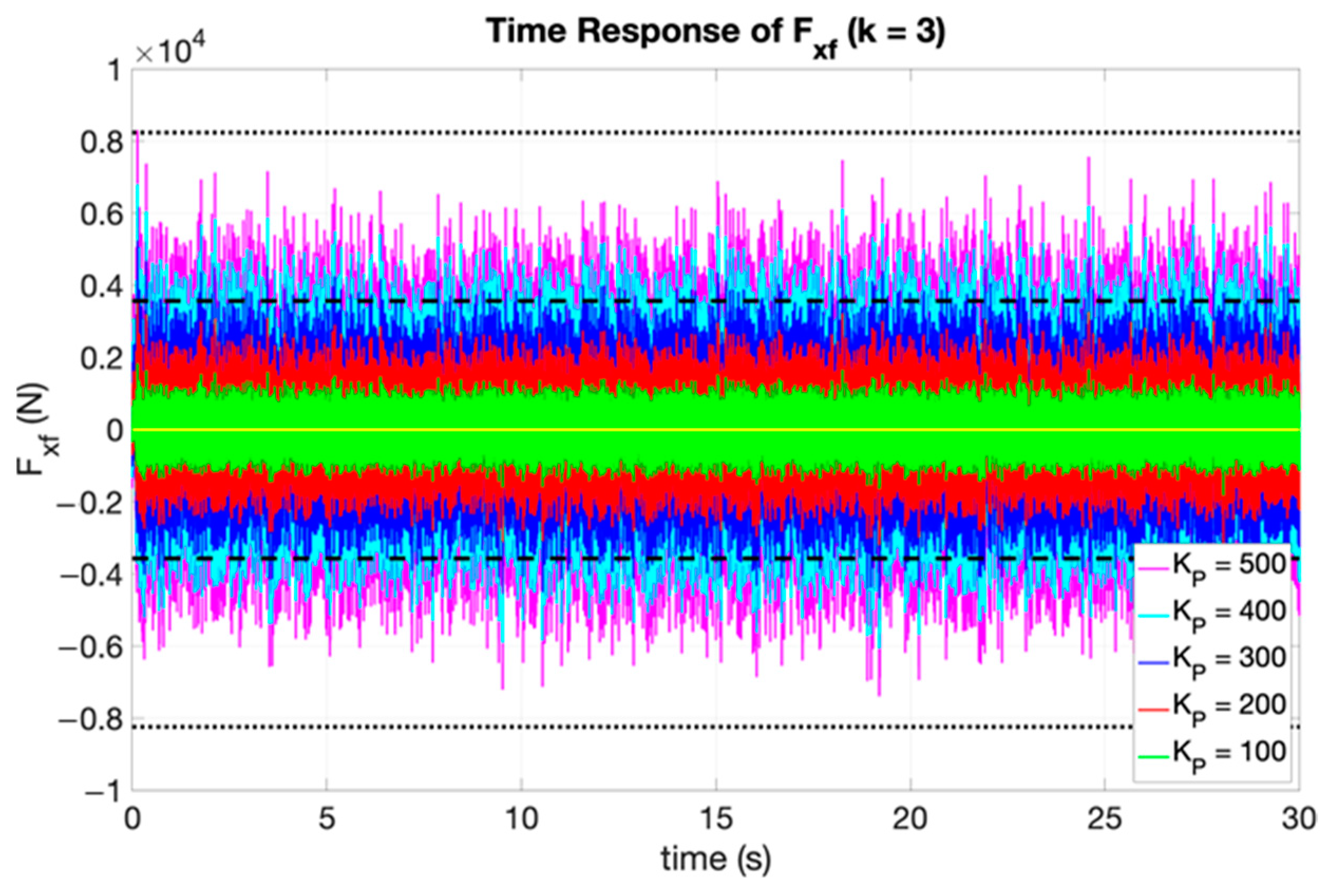
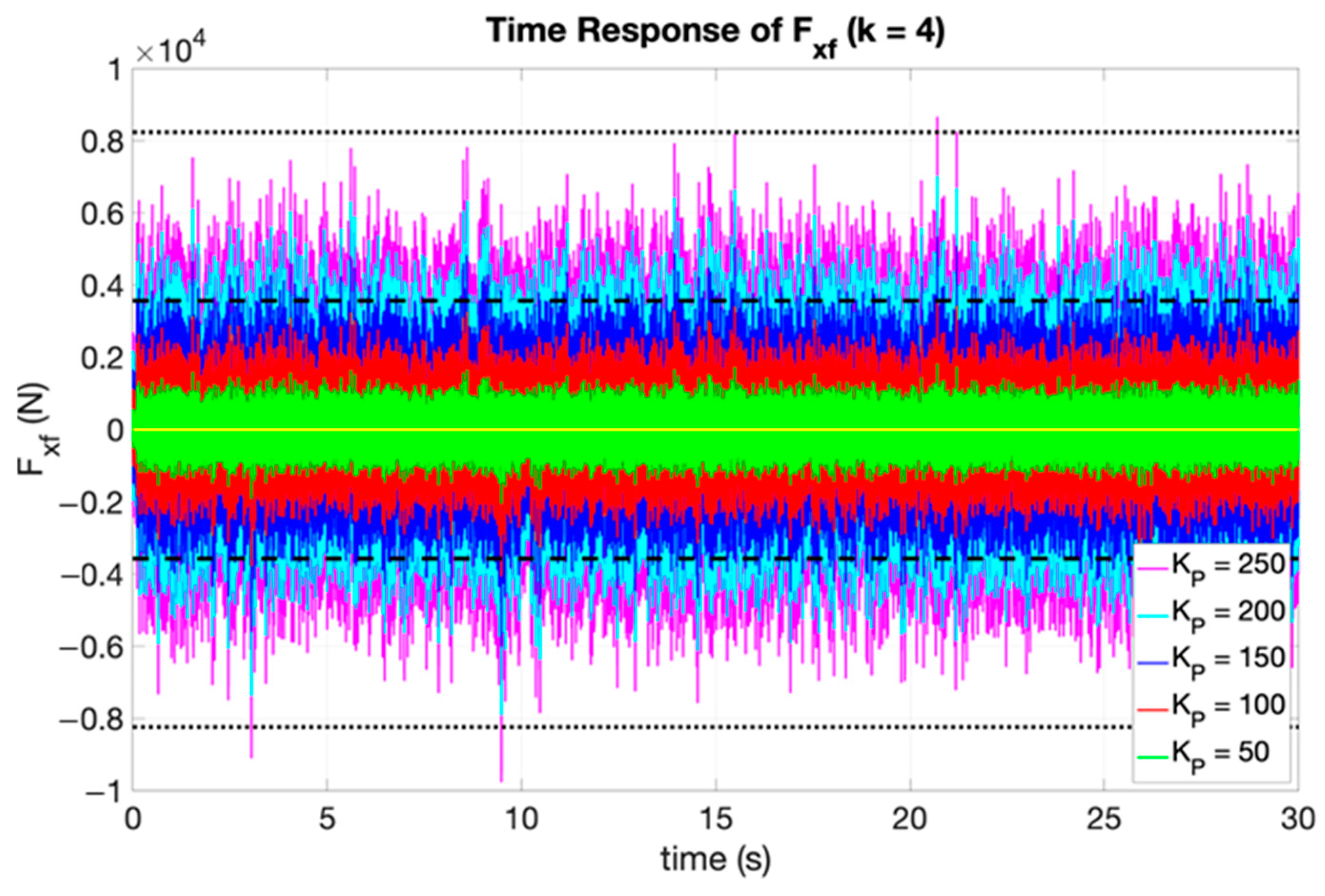
2.2. Vehicle Dynamics Model with Proportional Ride-Blending Controller

For the closed-loop system of the vehicle, the proportional ride-blending controller is implemented. The control law is defined as follows:

$$\begin{gathered} F_{xf}=K_p\left({\ddot{z}}_b-{\ddot{z}}_{b,ref}\right) \\ {F}_{xr}=-F_{xf} \end{gathered}$$

(27)

where $K_p$ is proportional gain. To improve the ride comfort, the vertical acceleration of the sprung mass should be minimized; therefore, the reference vertical acceleration of the sprung mass, ${\ddot{z}}_{b,ref}$, is set to zero. Additionally, $F_{xr}=-F_{xr}$ will not affect the velocity of the vehicle. Equation (27) will be

$$\begin{gathered} F_{xf}=K_p{\ddot{z}}_b \\ {F}_{xr}=-F_{xf} \end{gathered}$$

(28)

Once $F_{xf}$ and $F_{xr}$ are known, the front and rear vertical forces, $A_z$ and $B_z$, can be computed and used to control the vibration of the sprung mass. Then, the system is controlled by closed-loop control. The dynamics model of the closed-loop system is determined as follows: substitute Equations (1)–(4), (7)–(10), and (28) into Equations (5) and (6), and then the vehicle dynamics of the sprung mass are defined by

$$\begin{gathered} {\ddot{z}}_b=-{\displaystyle \frac{k_f+k_r}{M}}{z}_b-{\displaystyle \frac{c_f+c_r}{M}}{\dot{z}}_b+{\displaystyle \frac{{bk}_f-c{k}_r}{M}}\theta +{\displaystyle \frac{{bc}_f-{cc}_r}{M}} \dot{\theta } \\ +{\displaystyle \frac{k_f}{M}}{z}_f+{\displaystyle \frac{k_r}{M}}{z}_r+{\displaystyle \frac{c_f}{M}}{\dot{z}}_f+{\displaystyle \frac{c_r}{M}}{\dot{z}}_r \end{gathered}$$

(29)

where $M=m-K_P\left({\displaystyle \frac{e_f}{d_f}}+{\displaystyle \frac{e_r}{d_r}}\right)$.

$$\begin{array}{c}\ddot{\theta }={\displaystyle \frac{b{k}_f-c{k}_r+N(k_f+k_r)}{I_z}}{z}_b+{\displaystyle \frac{b{c}_f-c{c}_r+N(c_f+c_r)}{I_z}}{\dot{z}}_b\\ -{\displaystyle \frac{b^2{k}_f+c^2{k}_r+N(b{k}_f-c{k}_r)}{I_z}}\theta -{\displaystyle \frac{{b^{2}c}_f+c^2{c}_r+N(b{c}_f-c{c}_r)}{I_z}} \dot{\theta }\\ -{\displaystyle \frac{b{k}_f+N{k}_f}{I_z}}{z}_f+{\displaystyle \frac{{ck}_r-N{k}_r}{I_z}}{z}_r-{\displaystyle \frac{b{c}_f+N{c}_f}{I_z}}{\dot{z}}_f+{\displaystyle \frac{c{c}_r-N{c}_r}{I_z}}{\dot{z}}_r\end{array}$$

(30)

where $N={\displaystyle \frac{\left[-\left(h-\frac{b{e}_f}{d_f}\right)+\left(h-\frac{c{e}_r}{d_r}\right)\right]}{M}}{K}_P$.

Then, the state-space representation of the system is shown as follows:

$$\begin{array}{c}\dot{x}=A_{cl}x+B_{cl}u\\ y=C_{cl}x+D_{cl}u\end{array}$$

(31)

where $A_{cl}$, $B_{cl}$, $C_{cl}$, and $D_{cl}$ are defined in Appendix A, Equation (A4), and $x$ and $u$ are defined as follows:

$$\begin{array}{c}x={\left[\begin{array}{cccc}{z}_b& {\dot{z}}_b& \theta & \dot{\theta }\end{array}\right]}^T,\\ u={\left[\begin{array}{cccc}{z}_f& z_r& {\dot{z}}_f& {\dot{z}}_r\end{array}\right]}^T\end{array}$$

(32)

Since the format of the state-space representation of the closed-loop system in Equation (32) is the same as the format of the state-space representation of the open-loop system in Equation (14), the transfer function of the road input to the vertical acceleration of the sprung mass of the closed-loop system can be determined by the same steps as for the open-loop system in Equations (15)–(18). It is defined by Equation (33).

$${\displaystyle \frac{{\dot{Z}}_{b,cl}\left(s\right)}{Road\left(s\right)}}=G_{1,cl}{\left(s\right)}_{z_f\to {\dot{z}}_b}+G_{2,cl}{\left(s\right)}_{z_r\to {\dot{z}}_b}+G_{3,cl}{\left(s\right)}_{{\dot{z}}_f\to {\dot{z}}_b}+G_{4,cl}{\left(s\right)}_{{\dot{z}}_r\to {\dot{z}}_b}$$

(33)

$${\displaystyle \frac{{\ddot{Z}}_{b,cl}\left(s\right)}{Road\left(s\right)}}={\displaystyle \frac{{s\dot{Z}}_{b,cl}\left(s\right)}{Road\left(s\right)}}={\displaystyle \frac{s{\dot{Z}}_{b,cl}\left(s\right)}{Z_f\left(s\right)}}+{\displaystyle \frac{{e^{-\tau s}s\dot{Z}}_{b,cl}\left(s\right)}{Z_r\left(s\right)}}+{\displaystyle \frac{s^2{\dot{Z}}_{b,cl}\left(s\right)}{{\dot{Z}}_f\left(s\right)}}+{\displaystyle \frac{{e^{-\tau s}{s}^2\dot{Z}}_{b,cl}\left(s\right)}{{\dot{Z}}_r\left(s\right)}}$$

(34)

where

$${\displaystyle \frac{{\dot{Z}}_{b,cl}\left(s\right)}{Z_f\left(s\right)}}=C{\left(sI-A_{cl}\right)}^{-1}{B}_{cl}\left(:,1\right)+D\left(:,1\right)$$

(35)

$${\displaystyle \frac{{\dot{Z}}_{b,cl}\left(s\right)}{Z_r\left(s\right)}}=C{\left(sI-A_{cl}\right)}^{-1}{B}_{cl}\left(:,2\right)+D\left(:,2\right)$$

(36)

$${\displaystyle \frac{{\dot{Z}}_{b,cl}\left(s\right)}{{\dot{Z}}_f\left(s\right)}}=C{\left(sI-A_{cl}\right)}^{-1}{B}_{cl}\left(:,3\right)+D\left(:,3\right)$$

(37)

$${\displaystyle \frac{{\dot{Z}}_{b,cl}\left(s\right)}{{\dot{Z}}_r\left(s\right)}}=C{\left(sI-A_{cl}\right)}^{-1}{B}_{cl}\left(:,4\right)+D\left(:,4\right)$$

(38)

Using the parameters in Table 1, substitute them into Equations (32) and (35)–(38). Then, the transfer function of the road input to the vertical acceleration of the sprung mass can be calculated from Equation (34).

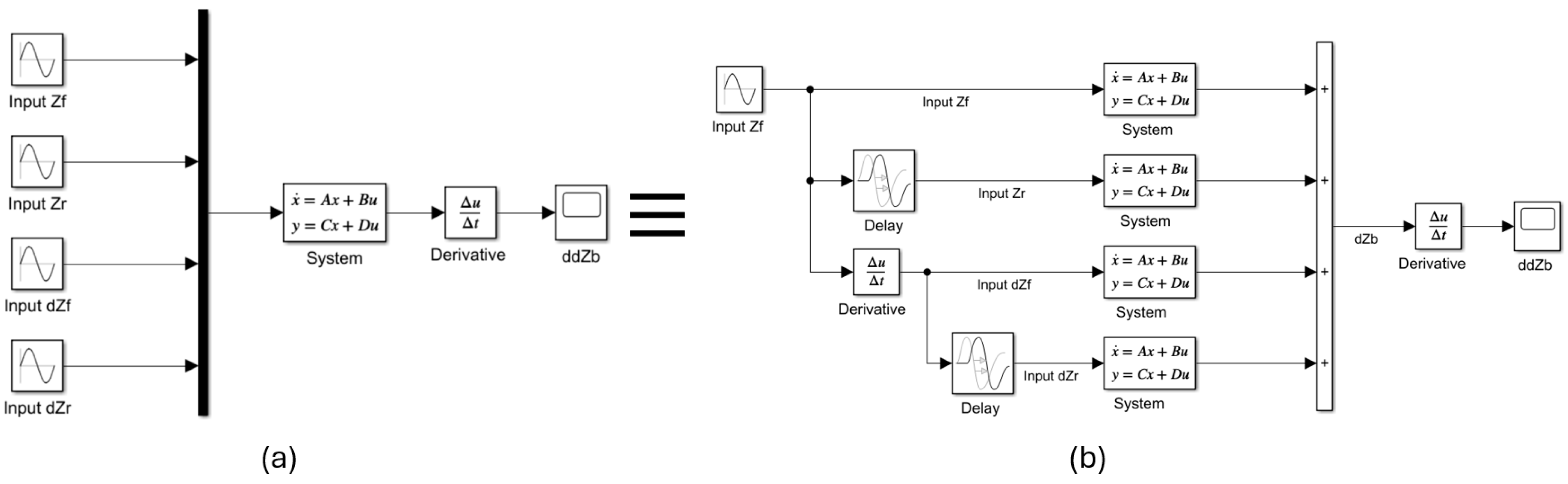
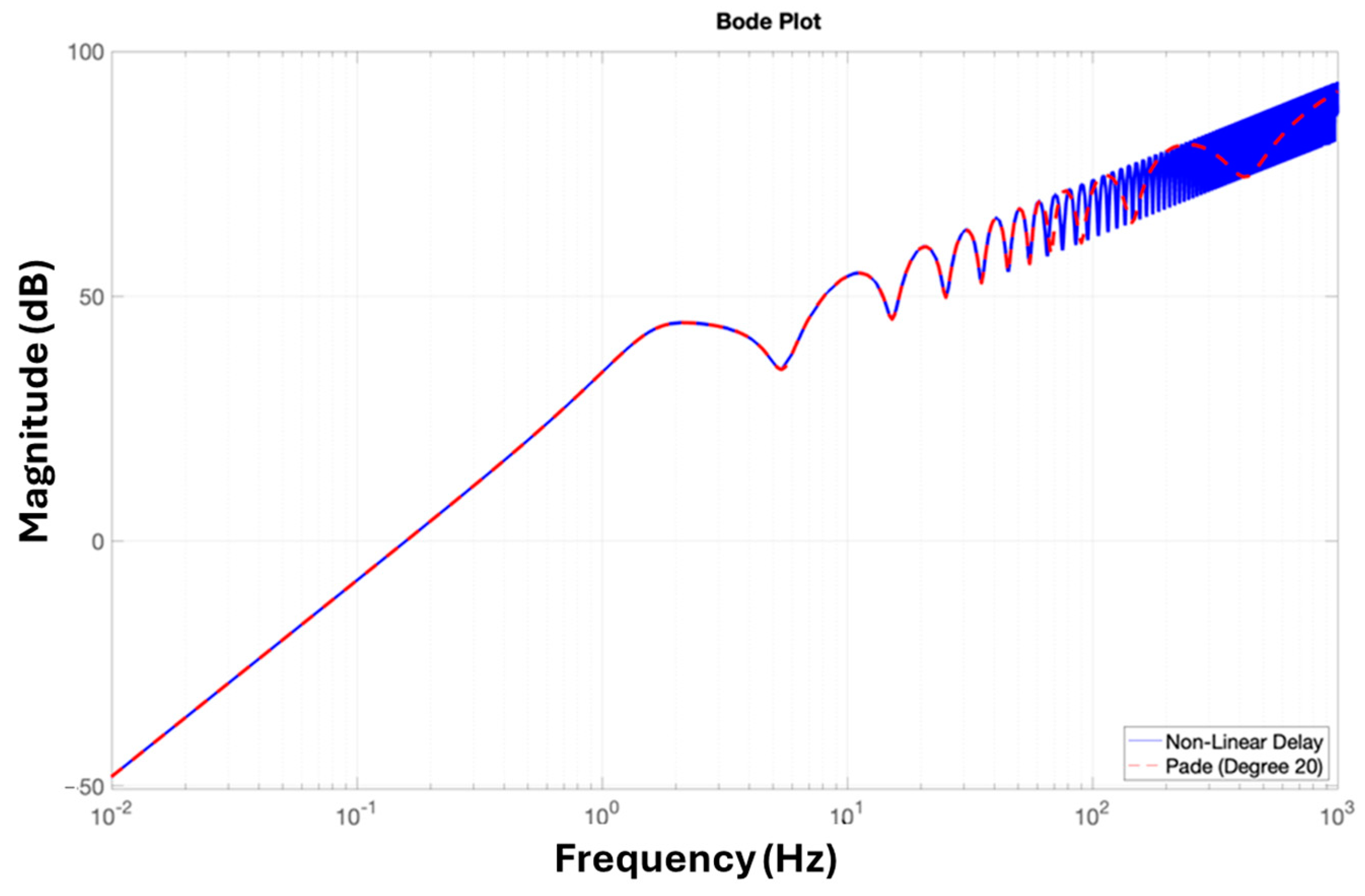
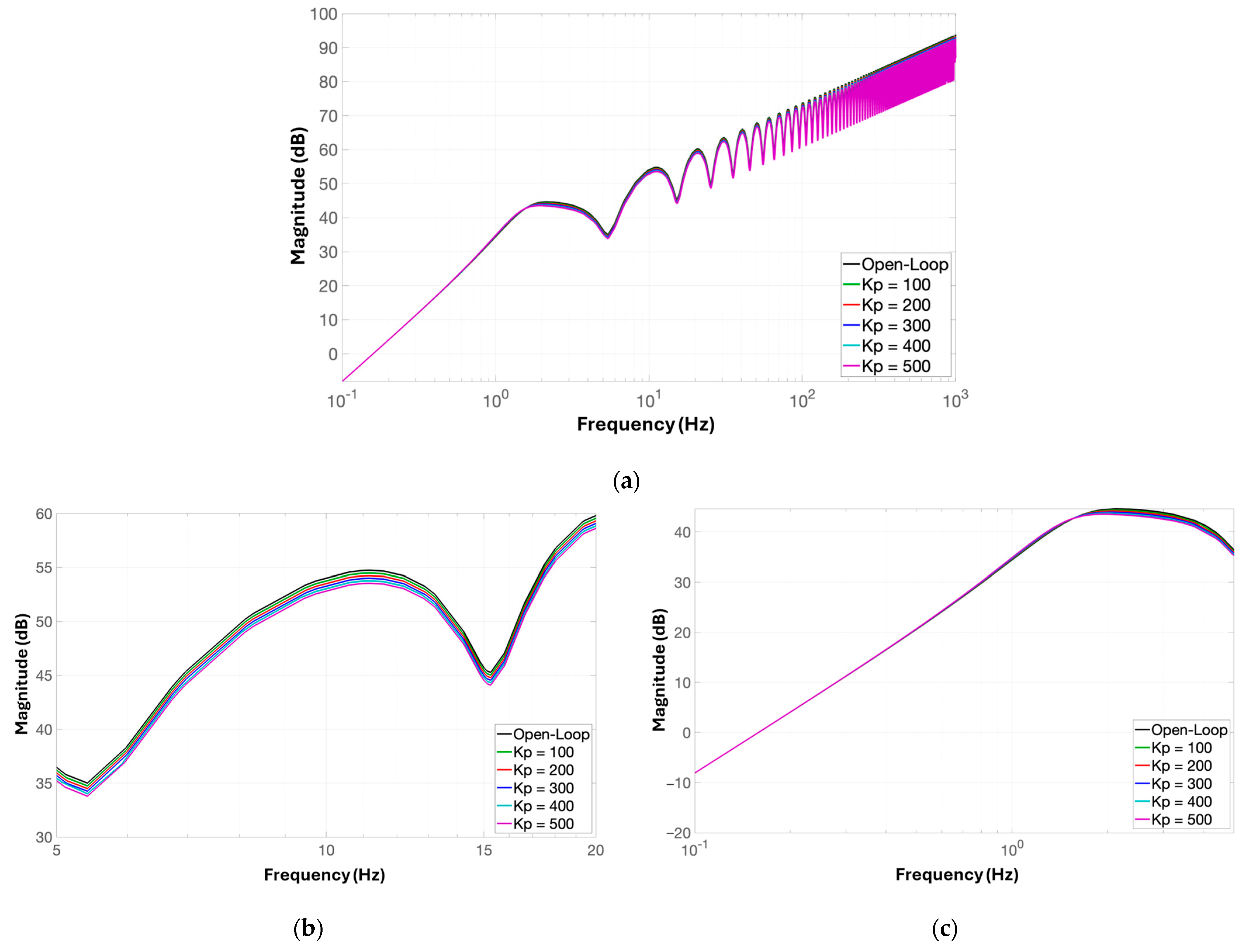
2.3. Frequency Response of the Vehicle System

Based on the transfer function of the road input to the vertical acceleration of the open-loop and closed-loop systems, as shown in Equations (18) and (34), the frequency response of both systems can be compared. To evaluate the frequency response, the velocity of the vehicle is assumed to be constant at 30 m/s. Given that the distance between the front and rear wheels is $b+c$, the delay time, $\tau$, of exact delay is 0.0991. The frequency response will be computed using MATLAB R2024a software [33]. An example of the frequency response of the open-loop system is shown in Figure 5.

Figure 5 compares the frequency response of the open-loop system when the delay time is modeled using the exact delay as in Equation (39) and approximated with the Pade approximation [34] with a Pade degree of 20. The figure shows that the frequency responses from both methods are the same up to a frequency of 60 Hz. Beyond 60 Hz, the frequency response from the Pade approximation cannot match the response from the exact delay. Therefore, the exact delay will be used for further evaluations in this case, even though it may be more complicated. The frequency response of the vehicle system is used to evaluate the system’s response at each frequency and to calculate the ride comfort for both systems.

Figure 6 shows the frequency response of both the open-loop and closed-loop systems. The proportional gain, $K_p$, is varied from 100 to 500 to present the frequency response of the closed-loop system. Figure 6a compares the frequency responses of the open-loop and closed-loop systems. Figure 6b,c provide zoomed-in views focusing on the frequency ranges of 5 to 20 Hz and 0.1 to 5 Hz, respectively. It can be seen from Figure 6 that as the proportional gain, $K_p$, increases, the amplitude response of the closed-loop system decreases compared to that of the open-loop system. Therefore, it can be concluded that the proportional ride-blending controller effectively reduces the vibration of the vehicle’s sprung mass.

2.4. Ride Comfort (ISO 2631)

According to ISO 2631 [30], ride comfort is the comfort reaction evaluated by examining the frequency-weighted acceleration, $a_w$. The frequency-weighted acceleration, $a_w$, is computed from the Power Spectral Density (PSD) of the sprung mass vertical acceleration, ${\ddot{z}}_b$. The equation for the frequency-weighted acceleration, $a_w$, is shown in Equation (39).

$$a_w=\sqrt{\sum _i{\left(W_i{a}_i\right)}^2}$$

(39)

where $W_i$ is frequency weighting in one-third-octaves for the frequency $i$ according to the Principal Frequency Weighting in One-Third-Octaves Table (parameter: $W_k)$ [35] and $a_i$ is root mean square (RMS) acceleration for the frequency, $i$, as shown in Equation (40).

$$a_i=\sqrt{P_i}$$

(40)

where $P_i$ is the area under the plot of Power Spectral Density (PSD) of the sprung mass vertical acceleration, ${\ddot{z}}_b$, for frequency $i$. Frequency $i$ is the range between $f_{i-\frac{1}{2}}$ and $f_{i+\frac{1}{2}}$ where $f_{i-\frac{1}{2}}=2^{(-\frac{1}{6})}{f}_i$ and $f_{i+\frac{1}{2}}=2^{(\frac{1}{6})}{f}_i$. (Note: the frequency according to one-third-octaves is defined by ${\displaystyle \frac{f_{n+1}}{f_n}}=2^{\frac{1}{3}}$.) The expanationtion of $P_i$ is shown in Figure 7.

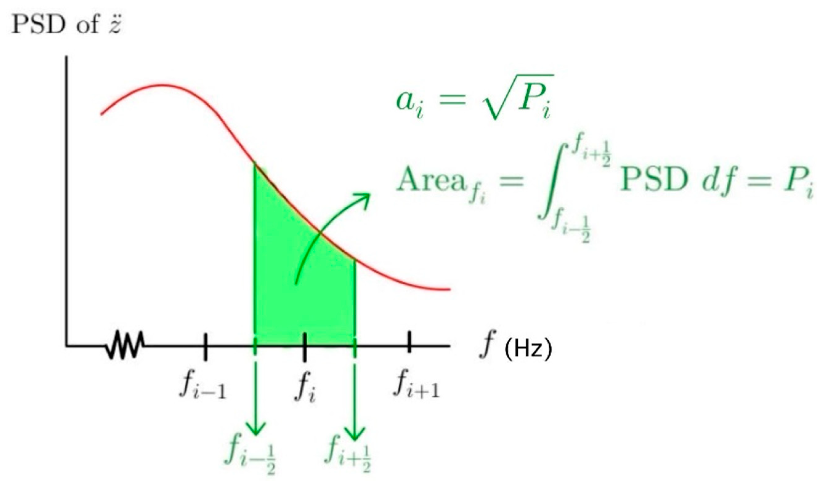
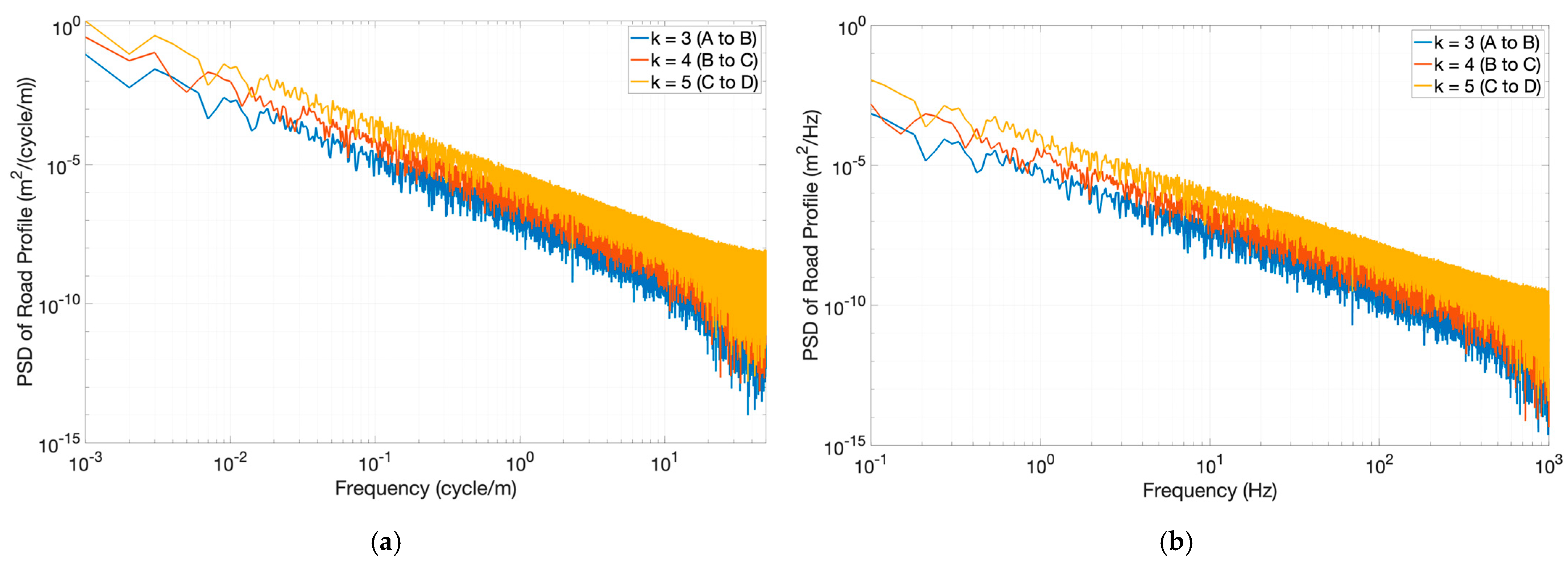
2.4.1. Power Spectral Density (PSD)

PSD is a measure of the power distribution of a signal over different frequencies. It shows how the power (or variance) of a time series is distributed with frequency, providing insights into the dominant frequencies present in the signal. To compute the PSD of the sprung mass vertical acceleration, ${\ddot{z}}_b$, the road profile input is supplied to the vehicle system or the transfer function as described in Equations (18) and (34). The system will generate an output, which will then be used to calculate the PSD of the vertical acceleration of the sprung mass. The PSD of the vertical acceleration of the sprung mass at frequency $i$ can be computed by Equation (41). An example of calculating the PSD of the vertical acceleration of the sprung mass is shown in Figure 8. The PSD of acceleration at frequency, $f$, is calculated from the PSD of road profile and the frequency response of the vehicle as shown by the red line in Figure 8.

$$P_{avg,i_{out}}={\int }_{-\frac{T}{2}}^{\frac{T}{2}}{{[A}_i\left|G\left({\omega }_{i}i\right)\right|\mathit{sin}{(\omega }_{i}t+{\varphi }_i+\angle G\left({\omega }_{i}i\right)\left)\right]}^{2}dt={\displaystyle \frac{{\left(A_i\left|G\left({\omega }_{i}i\right)\right|\right)}^2}{2}}$$

(41)

where $i$ is frequency, $G\left(s\right)$ is transfer function as described in Equations (18) and (34), and the road input at frequency $i$ is

$$z_i\left(t\right)=A_{i}sin(2\pi f_{i}t+{\varphi }_i)$$

(42)

The instantaneous power of road profile, $P_{avg}$, is

$$P_{avg}={\int }_{\frac{-T}{2}}^{\frac{T}{2}}P\left(t\right)dt={\int }_{\frac{-T}{2}}^{\frac{T}{2}}{z}_i^2\left(t\right)dt={\displaystyle \frac{A_i^2}{2}}$$

(43)

Equation (43) shows that $P_{avg}$ depends on the amplitude of the road profile as described in Equation (42).

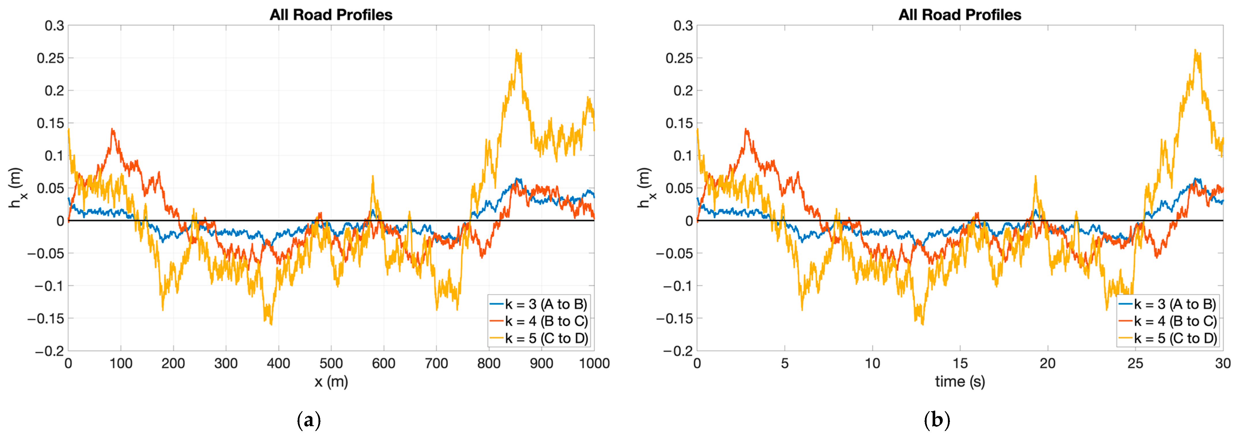
2.4.2. Classification of Roads (ISO 8608)

According to ISO 8608 [36,37], road profiles are classified based on the PSD of the road profile elevation, as shown in Figure 9. There are eight classes of road profiles: A, B, C, D, E, F, G, and H. The road profiles can be created by Equation (44) [38].

$$z\left(x\right)=\sum _{i=1}^N\sqrt{\Delta n}·2^k·{10}^{-3}·\left({\displaystyle \frac{n_0}{i·\Delta n}}\right)·\mathit{cos}\left(2\pi i·\Delta n·x+{\varphi }_i\right)$$

(44)

where $x$ is the horizontal displacement (0 to $L$), $∆n={\displaystyle \frac{1}{L}}$, $n_0=0.1 rad/s$, $N$ is number of the total data points, ${\varphi }_i$ is the random phase angle in the interval of 0 to $2\pi$, and $k$ is the constant to classify the road profile accoding to

Table 2. The relationship between $k$ and the class of road profile.

Class of Road Profile	$\mathit{k}$
A to B	3
B to C	4
C to D	5
D to E	6
E to F	7
F to G	8
G to H	9

. Examples of road profiles for classes A to D are shown in Figure 10. Ref. [29] indicates that class A represents a very good road, class B a good road, class C an average road, and class D a poor road. For this research, only classes A to D will be used to evaluate the control technique.

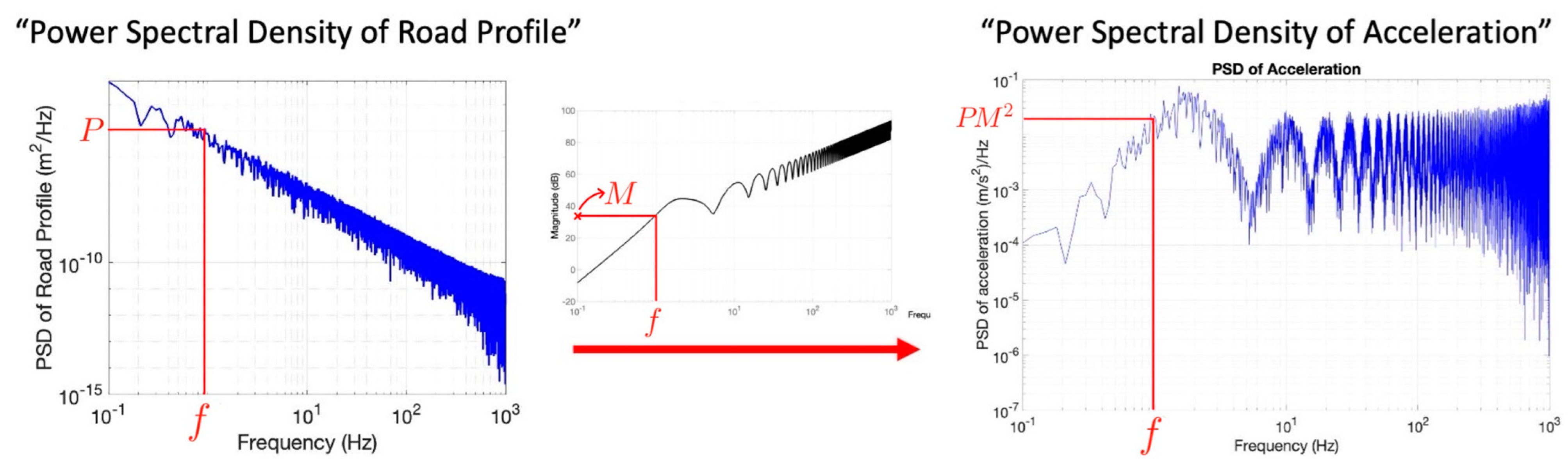
2.4.3. PSD of the Road Profiles

Three types of road profiles are created by Equation (44): (1) $k=3$: road profile class A to B; (2) $k=4$: road profile class B to C; and (3) $k=5$: road profile class C to D. Figure 11a shows the elevation of these three types of road profiles versus distance (x). Assuming that the vehicle velocity is constant at 30 m/s, Figure 11b presents the elevation of the three types of road profiles versus time over a 30 s period. This conversion is carried out using Equations (45) and (46). Equation (45) shows the relationship between spectral frequency and temporal frequency, while Equation (46) outlines the method for converting elevation from spectral frequency to temporal frequency.

$$f_{Spectral}=v{f}_{Temporal}$$

(45)

where $f_{Spectral}$ is spectral frequency (cycle/m), $f_{Temporal}$ is temporal frequency (cycle/s or Hz), and $v$ is velocity.

$$z_i\left(x\right)=A_{i}sin(2\pi f_{i}x+{\varphi }_i)\to z_i\left(t\right)=A_{i}sin(2\pi f_{i}t+{\varphi }_i)$$

(46)

Then, Figure 11 is used to calculate the PSD of the road profiles.

Figure 12 shows the PSD of the road profiles created by Figure 11. Figure 12a presents the PSD with the spatial frequency domain, while Figure 12b shows the PSD with the temporal frequency domain. The PSD is computed by the MATLAB software using the psd_1D function [39]. Figure 11b will be used to calculate the PSD of the sprung mass vertical acceleration, ${\ddot{z}}_b$, according to the method explaned in Figure 8.

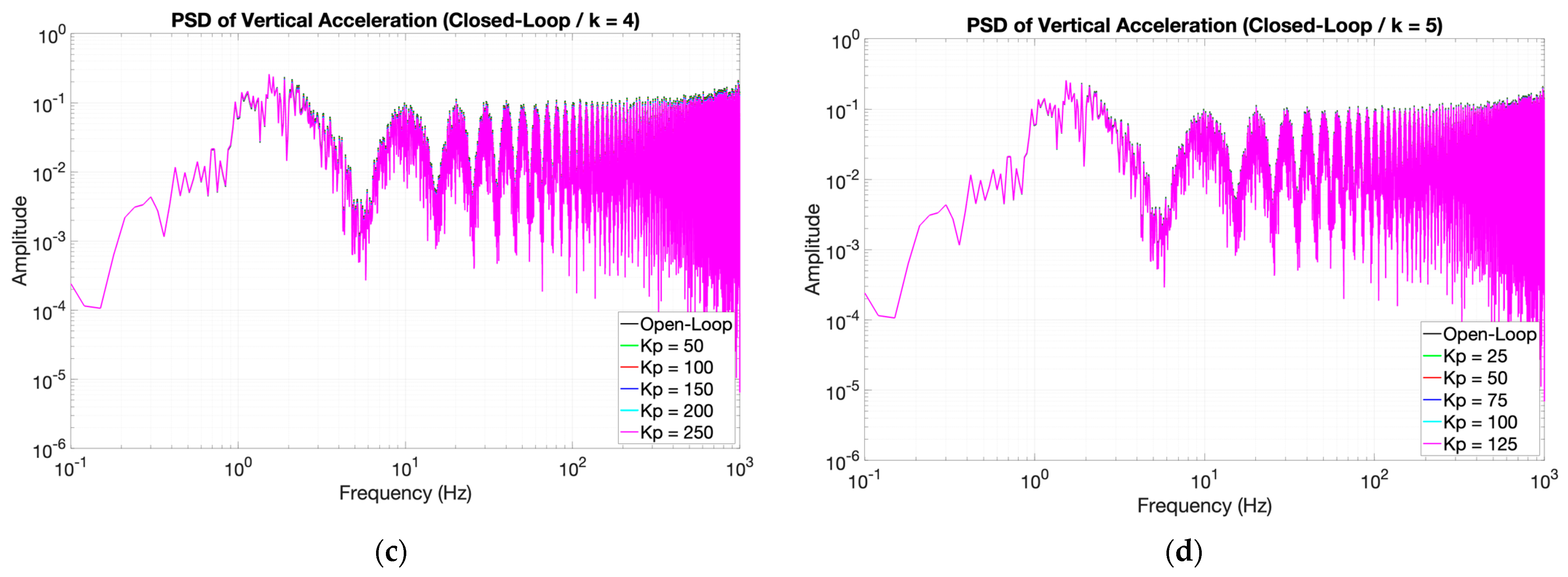
2.4.4. PSD of the Sprung Mass Vertical Acceleration

The PSD of the sprung mass vertical acceleration is calculated based on Equation (41) and Figure 8. The results are shown in Figure 13. Figure 13a presents the PSD of the open-loop system for road profile classes A to B, B to C, and C to D. Figure 13b compares the PSD of the open-loop and closed-loop systems for road profile classes A to B. Figure 13c compares the PSD of the open-loop and closed-loop systems for road profile classes B to C. Finally, Figure 13d compares the PSD of the open-loop and closed-loop systems for road profile classes C to D.

In the next section, the results of the frequency-weighted acceleration, $a_w$, are presented to compare the ride comfort.

3. Results and Discussion

3.1. Frequency Response of the Open-Loop and Closed-Loop System

The transfer functions of the open-loop and closed-loop systems, shown in Equations (18) and (34), are used to determine the frequency responses in Figure 6. The figure compares the frequency responses for both systems and demonstrates that increasing $K_p$ results in a reduced amplitude response in the closed-loop system compared to the open-loop system. This indicates that the proportional ride-blending controller effectively reduces the vibration of the vehicle’s sprung mass.

3.2. Frequency-Weighted Acceleration

The frequency-weighted acceleration, $a_w$, is an indicator used to evaluate ride comfort; lower values of the frequency-weighted acceleration correspond to better ride comfort. The frequency-weighted acceleration is calculated from Equations (39) and (40), based on the Power Spectral Density (PSD) of the sprung mass vertical acceleration, ${\ddot{z}}_b$, shown in Figure 13. Comparisons of the frequency-weighted acceleration for each type of road profile are presented in

Table 3. Proportional gain and frequency-weighted acceleration for road profile classes A to B.

$\mathbf{Proportional} \mathbf{Gain}, {\mathit{K}}_{\mathit{p}}$	Frequency-Weighted $\mathbf{Acceleration} ({\mathit{a}}_{\mathit{w}},\mathbf{m}/{\mathbf{s}}^2$)	Percentage Decrease (Compared with Open-Loop)
0 (Open-Loop)	0.3721	0%
100	0.3622	2.6641%
200	0.3528	5.1856%
300	0.3439	7.5756%
400	0.3355	9.8441%
500	0.3275	12.000%

,

Table 4. Proportional gain and frequency-weighted acceleration for road profile classes B to C.

$\mathbf{Proportional} \mathbf{Gain}, {\mathit{K}}_{\mathit{p}}$	Frequency-Weighted $\mathbf{Acceleration} ({\mathit{a}}_{\mathit{w}},\mathbf{m}/{\mathbf{s}}^2$)	Percentage Decrease (Compared with Open-Loop)
0 (Open-Loop)	0.7349	0%
50	0.7250	1.3583%
100	0.7153	2.6789%
150	0.7058	3.9632%
200	0.6966	5.2127%
250	0.6877	6.4288%

and

Table 5. Proportional gain and frequency-weighted acceleration for road profile classes C to D.

$\mathbf{Proportional} \mathbf{Gain}, {\mathit{K}}_{\mathit{p}}$	Frequency-Weighted $\mathbf{Acceleration} ({\mathit{a}}_{\mathit{w}},\mathbf{m}/{\mathbf{s}}^2$)	Percentage Decrease (Compared with Open-Loop)
0 (Open-Loop)	1.4884	0%
25	1.4783	0.6800%
50	1.4683	1.3506%
75	1.4585	2.0119%
100	1.4488	2.6641%
125	1.4392	3.3073%

. Table 3 shows the frequency-weighted acceleration for road profile classes A to B, Table 4 for road profile classes B to C, and Table 5 for road profile classes C to D.

Table 6. The root mean square (RMS) of the vertical acceleration of the sprung mass for the road profile classes A to B.

$\mathbf{Proportional} \mathbf{Gain}, {\mathit{K}}_{\mathit{p}}$	$\mathbf{RMS} \mathbf{of} {\ddot{\mathit{z}}}_{\mathit{b}}$$(\mathbf{m}/{\mathbf{s}}^2)$
0 (Open-Loop)	4.130
100	4.014
200	3.904
300	3.800
400	3.702
500	3.609

,

Table 7. The root mean square (RMS) of the vertical acceleration of the sprung mass for the road profile classes B to C.

$\mathbf{Proportional} \mathbf{Gain}, {\mathit{K}}_{\mathit{p}}$	$\mathbf{RMS} \mathbf{of} {\ddot{\mathit{z}}}_{\mathit{b}}$$(\mathbf{m}/{\mathbf{s}}^2)$
0 (Open-Loop)	8.269
50	8.151
100	8.037
150	7.925
200	7.817
250	7.712

and

Table 8. The root mean square (RMS) of the vertical acceleration of the sprung mass for the road profile classes C to D.

$\mathbf{Proportional} \mathbf{Gain}, {\mathit{K}}_{\mathit{p}}$	$\mathbf{RMS} \mathbf{of} {\ddot{\mathit{z}}}_{\mathit{b}}$$(\mathbf{m}/{\mathbf{s}}^2)$
0 (Open-Loop)	16.52
25	16.40
50	16.28
75	16.17
100	16.05
125	15.94

show that as the proportional gain ($K_p$) increases, the frequency-weighted acceleration ($a_w$) decreases, leading to enhanced ride comfort. This indicates that the method of controlling the driving force from the IWM using the proportional ride-blending controller, as discussed in Section 2.2, effectively reduces the vehicle’s vibration. The decrease in $a_w$ is directly correlated with the increase in $K_p$.

3.3. Frequency-Weighted Acceleration

Based on the IWM L1500 information in Figure 14, the wheel forces are limited. Figure 15, Figure 16 and Figure 17 illustrate examples of the front wheel forces based on the proportional ride-blending controller as defined in Equation (28). These figures show the time response of the front wheel forces over the first 30 s for each type of road profile (classes A to B, B to C, and C to D) and for a variety of proportional gains. The black dashed lines represent the maximum continuous force limit of 3570 N, while the black dotted lines represent the maximum peak force limit of 8240 N, according to the parameters in Figure 14 (The yellow line in Figure 15, Figure 16 and Figure 17 is the reference force, zero newtons). Moreover, the root mean square (RMS) of the vertical acceleration of the sprung mass, corresponding to various proportional gains and types of road profiles, is shown in Table 6, Table 7 and Table 8.

Table 6, Table 7 and Table 8 demonstrate that increasing the proportional gains reduces the RMS of the vertical acceleration of the sprung mass, or the frequency-weighted acceleration. Conversely, Figure 15, Figure 16 and Figure 17 illustrate that higher proportional gains lead to an increase in the front wheel driving forces of the IWM.

Considering the time response of the front wheel driving forces for the road profile classes A to B in Figure 15, with $K_p=300$, the blue line indicates that most of the driving forces are within the continuous force limit, and the peak forces are within the peak force limit. Thus, $K_p=300$ is suitable for this case, resulting in an improvement of up to 7.58% in frequency-weighted acceleration compared to the open-loop system.

Similarly, for the road profile classes B to C in Figure 16, with $K_p=150$, the blue line shows that most of the driving forces are within the continuous force limit, and the peak forces are within the peak force limit. Therefore, $K_p=150$ is appropriate for this case, resulting in an improvement of up to 3.96% in frequency-weighted acceleration compared to the open-loop system.

Additionally, considering the time response of the front wheel driving forces for the road profile classes C to D in Figure 17, with $K_p=75$, the blue line indicates that most of the driving forces are within the continuous force limit, and the peak forces are within the peak force limit. Thus, $K_p=75$ is suitable for this situation, resulting in an improvement of up to 2.01% in frequency-weighted acceleration compared to the open-loop system.

In summary, the closed-loop systems with the proportional ride-blending controller for the IWM effectively reduce the frequency-weighted acceleration, as per ISO 2631, and the RMS of the vertical acceleration of the sprung mass. The results demonstrate that increasing the proportional gain decreases both the frequency-weighted acceleration and the RMS of the vertical acceleration of the sprung mass. However, due to the torque limitations of the IWMs, excessively high proportional gains may prevent the motors from generating sufficient torque and force to reduce the vertical acceleration effectively.

Table 9. The summary of the appropriate value of $K_P$ for each type of road profile.

Type of Road Profile	The Most Appropriate $\mathbf{Value} \mathbf{of} {\mathit{K}}_{\mathit{P}}$	Percentage Decrease in Frequency-Weighted Acceleration (Compared with Open-Loop)
k = 3 (Class A to B)	300	7.5756%
k = 4 (Class B to C)	150	3.9632%
k = 5 (Class C to D)	75	2.0119%

summarizes the suitable proportional gains for each type of road profile and shows the corresponding percentage reduction in frequency-weighted acceleration. To achieve optimal reduction, an adaptive proportional gain controller based on the values in Table 9 may be implemented to maximize the decrease in frequency-weighted acceleration.

4. Conclusions

This study investigated the impact of vertical force control in IWMs on enhancing ride comfort in electric vehicles (EVs) using a dynamic vehicle model and a proportional ride-blending controller. The implementation and analysis of the system’s frequency response demonstrated that the proportional ride-blending controller effectively reduces vertical vibrations of the sprung mass, thereby improving ride comfort.

This research converted the state-space model into a transfer function to evaluate the system’s response. Road profiles were generated according to ISO 8608 standards and converted into Power Spectral Density (PSD) inputs for simulation. The frequency-weighted acceleration ($a_w$) was calculated based on ISO 2631 standards to assess ride comfort improvements. The findings revealed that increasing the proportional gain ($K_p$) reduced both the frequency-weighted acceleration and the RMS of the vertical acceleration of the sprung mass. However, due to the torque limitations of the IWMs, the gain could not be increased indefinitely.

In summary, this study provides a comprehensive analysis of using vertical force control in IWMs to enhance ride comfort in EVs. The results suggest that advanced suspension technologies, including the proportional ride-blending controller, can effectively address the challenges posed by increased unsprung mass in IWM vehicles, offering a promising approach to improve ride quality and vehicle dynamics.

References

1. Kopylov, S.; Phanomchoeng, G.; Ambrož, M.; Petan, Ž.; Kunc, R.; Qiu, Y. Improvements to a vehicle’s ride comfort by controlling the vertical component of the driving force based on in-wheel motors. J. Vib. Control 2023, 29, 4001–4014. [Google Scholar] [CrossRef]
2. Murata, S. Innovation by in-wheel-motor drive unit. Veh. Syst. Dyn. 2012, 50, 807–830. [Google Scholar] [CrossRef]
3. Ricciardi, V.; Ivanov, V.; Dhaens, M.; Vandersmissen, B.; Geraerts, M.; Savitski, D.; Augsburg, K. Ride blending control for electric vehicles. World Electr. Veh. J. 2019, 10, 36. [Google Scholar] [CrossRef]
4. Ma, Y.; Deng, Z.; Xie, D. Control of the active suspension for in-wheel motor. J. Adv. Mech. Des. Syst. Manuf. 2013, 7, 535–543. [Google Scholar] [CrossRef]
5. Liu, M.; Gu, F.; Zhang, Y. Ride comfort optimization of in-wheel-motor electric vehicles with in-wheel vibration absorbers. Energies 2017, 10, 1647. [Google Scholar] [CrossRef]
6. Savaresi, S.M.; Poussot-Vassal, C.; Spelta, C.; Sename, O.; Dugard, L. Semi-Active Suspension Control Design for Vehicles; Elsevier: Amsterdam, The Netherlands, 2010. [Google Scholar]
7. Zhu, S.; Tang, H. Simulation of magneto-rheological semi-active suspension system of EV driven by in-wheel motor. In Proceedings of the 3rd International Conference on Mechatronics, Robotics and Automation, Shenzhen, China, 20–21 April 2015; Atlantis Press: Dordrecht, The Netherlands, 2015; pp. 265–271. [Google Scholar]
8. Nie, S.; Zhuang, Y.; Chen, F.; Wang, Y.; Liu, S. A method to eliminate unsprung adverse effect of in-wheel motor-driven vehicles. J. Low Freq. Noise Vib. Act. Control 2018, 37, 955–976. [Google Scholar] [CrossRef]
9. Anaya-Martinez, M.; Lozoya-Santos, J.D.J.; Félix-Herrán, L.C.; Tudon-Martinez, J.C.; Ramirez-Mendoza, R.A.; Morales-Menendez, R. Control of automotive semi-active MR suspensions for in-wheel electric vehicles. Appl. Sci. 2020, 10, 4522. [Google Scholar] [CrossRef]
10. Liu, M.; Gu, F.; Huang, J.; Wang, C.; Cao, M. Integration design and optimization control of a dynamic vibration absorber for electric wheels with in-wheel motor. Energies 2017, 10, 2069. [Google Scholar] [CrossRef]
11. Shao, X.; Naghdy, F.; Du, H. Enhanced ride performance of electric vehicle suspension system based on genetic algorithm optimization. In Proceedings of the 2017 20th International Conference on Electrical Machines and Systems (ICEMS), Sydney, Australia, 11–14 August 2017; IEEE: Piscataway, NJ, USA, 2017; pp. 1–6. [Google Scholar]
12. Ma, Y.; Lu, C.; Zhao, H.; Hao, M. Nonlinear model predictive slip control based on vertical suspension system for an in-wheel-motored electric vehicle. In Proceedings of the 2017 29th Chinese Control And Decision Conference (CCDC), Chongqing, China, 28–30 May 2017; IEEE: Piscataway, NJ, USA, 2017; pp. 4967–4972. [Google Scholar]
13. Liu, M.; Zhang, Y.; Huang, J.; Zhang, C. Optimization control for dynamic vibration absorbers and active suspensions of in-wheel-motor-driven electric vehicles. Proc. Inst. Mech. Eng. Part D J. Automob. Eng. 2020, 234, 2377–2392. [Google Scholar] [CrossRef]
14. Fang, Z.; Liang, J.; Tan, C.; Tian, Q.; Pi, D.; Yin, G. Enhancing robust driver assistance control in distributed drive electric vehicles through integrated AFS and DYC technology. IEEE Trans. Intell. Veh. 2024. early access. [Google Scholar] [CrossRef]
15. Fang, Z.; Han, D.; Wang, J.; Wei, W.; Pi, D.; Yin, G. A Nash-equilibrium-based AFS-TVA Coordinated Control System for Distributed Drive Electric Vehicles Considering Safety and Energy. IEEE Trans. Transp. Electrif. 2024. early access. [Google Scholar] [CrossRef]
16. Jastrzębski, Ł.; Sapiński, B. Experimental investigation of an automotive magnetorheological shock absorber. Acta Mech. Autom. 2017, 11, 253–259. [Google Scholar] [CrossRef]
17. Zou, J.; Guo, X.; Abdelkareem, M.A.; Xu, L.; Zhang, J. Modelling and ride analysis of a hydraulic interconnected suspension based on the hydraulic energy regenerative shock absorbers. Mech. Syst. Signal Process. 2019, 127, 345–369. [Google Scholar] [CrossRef]
18. Tang, X.; Lin, T.; Zuo, L. Design and optimization of a tubular linear electromagnetic vibration energy harvester. IEEE/ASME Trans. Mechatron. 2013, 19, 615–622. [Google Scholar] [CrossRef]
19. Kopylov, S.; Chen, Z.B.; Abdelkareem, M.A. Acceleration based ground-hook control of an electromagnetic regenerative tuned mass damper for automotive application. Alex. Eng. J. 2020, 59, 4933–4946. [Google Scholar] [CrossRef]
20. Jin, X.; Wang, J.; Yang, J. Development of Robust Guaranteed Cost Mixed Control System for Active Suspension of In-Wheel-Drive Electric Vehicles. Math. Probl. Eng. 2022, 4628539. [Google Scholar] [CrossRef]
21. Ahmad, I.; Ge, X.; Han, Q.L. Decentralized dynamic event-triggered communication and active suspension control of in-wheel motor driven electric vehicles with dynamic damping. IEEE/CAA J. Autom. Sin. 2021, 8, 971–986. [Google Scholar] [CrossRef]
22. Jin, X.; Wang, J.; Sun, S.; Li, S.; Yang, J.; Yan, Z. Design of Constrained Robust Controller for Active Suspension of In-Wheel-Drive Electric Vehicles. Mathematics 2021, 9, 249. [Google Scholar] [CrossRef]
23. Long, G.; Ding, F.; Zhang, N.; Zhang, J.; Qin, A. Regenerative active suspension system with residual energy for in-wheel motor driven electric vehicle. Appl. Energy 2020, 260, 114180. [Google Scholar] [CrossRef]
24. Zhang, J.; Yang, Y.; Hu, M.; Fu, C.; Zhai, J. Model Predictive Control of Active Suspension for an Electric Vehicle Considering Influence of Braking Intensity. Appl. Sci. 2021, 11, 52. [Google Scholar] [CrossRef]
25. Ahmad, I.; Ge, X.; Han, Q.L. Communication-constrained active suspension control for networked in-wheel motor-driven electric vehicles with dynamic dampers. IEEE Trans. Intell. Veh. 2022, 7, 590–602. [Google Scholar] [CrossRef]
26. Yatak, M.Ö.; Şahin, F. Ride comfort-road holding trade-off improvement of full vehicle active suspension system by interval type-2 fuzzy control. Eng. Sci. Technol. Int. J. 2021, 24, 259–270. [Google Scholar] [CrossRef]
27. Wu, H.; Zheng, L.; Li, Y.; Zhang, Z.; Yu, Y. Robust Control for Active Suspension of Hub-Driven Electric Vehicles Subject to in-Wheel Motor Magnetic Force Oscillation. Appl. Sci. 2020, 10, 3929. [Google Scholar] [CrossRef]
28. Kissai, M.; Monsuez, B.; Tapus, A. Review of integrated vehicle dynamics control architectures. In Proceedings of the 2017 European Conference on Mobile Robots (ECMR), Paris, France, 6–8 September 2017; IEEE: Piscataway, NJ, USA, 2017; pp. 1–8. [Google Scholar]
29. Múčka, P. Simulated road profiles according to ISO 8608 in vibration analysis. J. Test. Eval. 2018, 46, 405–418. [Google Scholar] [CrossRef]
30. Min-Soo, P.A.R.K.; Fukuda, T.; Kim, T.G.; Maeda, S. Health risk evaluation of whole-body vibration by ISO 2631-5 and ISO 2631-1 for operators of agricultural tractors and recreational vehicles. Ind. Health 2013, 51, 364–370. [Google Scholar]
31. Katsuyama, E. Decoupled 3D moment control using in-wheel motors. Veh. Syst. Dyn. 2013, 51, 18–31. [Google Scholar] [CrossRef]
32. Hott, L.; Ivanov, V.; Augsburg, K.; Ricciardi, V.; Dhaens, M.; Al Sakka, M.; Praet, K.; Molina, J.V. Ride blending control for awd electric vehicle with in-wheel motors and electromagnetic suspension. In Proceedings of the 2020 IEEE Vehicle Power and Propulsion Conference (VPPC), Virtual, 18 November–16 December 2020; IEEE: Piscataway, NJ, USA, 2020; pp. 1–5. [Google Scholar]
33. The MathWorks Inc. Matlab. Available online: https://www.mathworks.com (accessed on 30 June 2024).
34. Andrianov, I.; Shatrov, A. Padé Approximants, Their Properties, and Applications to Hydrodynamic Problems. Symmetry 2021, 13, 1869. [Google Scholar] [CrossRef]
35. Medina Santiago, A.; Orozco Torres, J.A.; Hernández Gracidas, C.A.; Garduza, S.H.; Franco, J.D. Diagnosis and Study of Mechanical Vibrations in Cargo Vehicles Using ISO 2631-1:1997. Sensors 2023, 23, 9677. [Google Scholar] [CrossRef] [PubMed]
36. Múčka, P.; Stein, G.J.; Tobolka, P. Whole-body vibration and vertical road profile displacement power spectral density. Veh. Syst. Dyn. 2020, 58, 630–656. [Google Scholar] [CrossRef]
37. Múčka, P. Passenger car vibration dose value prediction based on ISO 8608 road surface profiles. SAE Int. J. Veh. Dyn. Stab. NVH 2021, 5, 425–441. [Google Scholar] [CrossRef]
38. Agostinacchio, M.; Ciampa, D.; Olita, S. The vibrations induced by surface irregularities in road pavements—A Matlab® approach. Eur. Transp. Res. Rev. 2014, 6, 267–275. [Google Scholar] [CrossRef]
39. Kanafi, M.M. 1-Dimensional Surface Roughness Power Spectrum of a Profile or Topography. MATLAB Central File Exchange 2020. Available online: https://www.mathworks.com/matlabcentral/fileexchange/54315-1-dimensional-surface-roughness-power-spectrum-of-a-profile-or-topography (accessed on 20 July 2024).
Figure 1. A half-vehicle dynamics model.
Applsci 14 06582 g001
Figure 2. Free body diagram of the half-vehicle model: (a) free body diagram of front and rear wheels; (b) free body diagram of sprung mass.
Applsci 14 06582 g002
Figure 3. Schematic diagram of the input for the vehicle system.
Applsci 14 06582 g003
Figure 4. Block diagram of the vehicle system: (a) block diagram with MISO system principle; (b) block diagram with linear combination principle.
Applsci 14 06582 g004
Figure 5. The frequency response of open-loop system by the exact delay and Pade approximation methods.
Applsci 14 06582 g005
Figure 6. The frequency response of open-loop and closed-loop system: (a) the frequency response from 0.1 to 1000 Hz, (b) the frequency response from 5 to 20 Hz, and (c) the frequency response from 0.1 to 5 Hz.
Applsci 14 06582 g006
Figure 7. The calculation of P i .
Applsci 14 06582 g007
Figure 8. The example of PSD conversion via Bode plot.
Applsci 14 06582 g008
Figure 9. Road profile classification according to ISO 8608 [36,37].
Applsci 14 06582 g009
Figure 10. Examples of road profiles for classes A to D: (a) class A, (b) class B, (c) class C, and (d) class D.
Applsci 14 06582 g010
Figure 11. The road profiles created by Equation (44): (a) the road profiles’ elevation versus distance (x); (b) the road profiles’ elevation versus time.
Applsci 14 06582 g011
Figure 12. PSD of the road profiles: (a) PSD with spatial frequency domain; (b) PSD with temporal frequency domain.
Applsci 14 06582 g012
Figure 13. PSD of the sprung mass vertical acceleration: (a) PSD of the open-loop system, (b) PSD of the closed-loop system for road profile classes A to B, (c) PSD of the closed-loop system for road profile classes B to C, and (d) PSD of the closed-loop system for road profile classes C to D.
Applsci 14 06582 g013aApplsci 14 06582 g013b
Figure 14. Parameters of the IWM L1500 [1].
Applsci 14 06582 g014
Figure 15. Time response of the front wheel force for the road profile classes A to B.
Applsci 14 06582 g015
Figure 16. Time response of the front wheel force for the road profile classes B to C.
Applsci 14 06582 g016
Figure 17. Time response of the front wheel force for the road profile classes C to D.
Applsci 14 06582 g017