Article

Performance of Strengthened Accelerated Oscillator Damper for Vibration Control of Bridges

1
School of Infrastructure Engineering, Dalian University of Technology, Dalian 116024, China
2
Longjian Road and Bridge Company Limited, Harbin 150028, China
*
Author to whom correspondence should be addressed.
Appl. Sci. 2024, 14(15), 6732; https://doi.org/10.3390/app14156732
Submission received: 18 July 2024 / Revised: 29 July 2024 / Accepted: 30 July 2024 / Published: 1 August 2024
(This article belongs to the Special Issue Advanced Technologies in Seismic Design, Assessment and Retrofitting)

Abstract

:
Vibration control has emerged as a significant concern in civil engineering, aiming to minimize the displacement and stress exerted on structures during seismic events. The accelerated oscillator damper (AOD), which is a damping device that depends on acceleration, has been demonstrated to be highly effective. However, in the case of traditional bridges, it is difficult to accurately place the secondary mass, spring, and damping components at the piers. Additionally, it has been found that as a general single-degree-of-freedom (SDOF) damping device, a significant limitation of the AOD system is its insufficient damping effect in the near-resonance region. This study presents a strengthened AOD with a liner spring (SAOD-LS), in which the secondary spring and damper are linked to the primary structure rather than being attached to the piers. This design not only provides enough space for the secondary system but also has a higher amplification factor of secondary spring and damping components compared with the original layout. In addition, we suggest a nonlinear spring device (NSD) that includes connecting rods and inclined linear springs arranged in a diamond configuration. This innovative design is intended to introduce nonlinear stiffness characteristics into the equivalent stiffness, thereby improving the device’s performance and providing effective anti-resonance features in the near-resonance region. We have confirmed the motion equations for the SAOD-LS and used finite element (FE) analysis to validate the formulation of the equivalent external force and deformation of the NSD. We have thoroughly investigated both the SAOD-LS and the strengthened AOD equipped with NSD as the secondary spring (SAOD-NSD) for their potential implementation in a bridge project. These damping systems demonstrate exceptional performance and robustness, making them highly suitable for enhancing structural resistance to seismic activity.

1. Introduction

In the past, there have been significant advancements in the fields of transportation engineering safety and civil engineering safety [1,2,3,4]. There is significant concern about the seismic safety of structures built in earthquake-prone regions [5,6]. To mitigate the negative impacts of seismic activities on human life and productivity, numerous technologies concerning vibration control have been extensively developed. Vibration control techniques play a significant role in reducing displacement and force response when subjected to seismic [7], ice [8], wind [9], and other types of loads. Recent trends in civil engineering have led to a proliferation of studies focusing on the damping effects of spring-mass-damper systems [10,11,12,13,14,15,16]. The approach of [17], namely the tuned mass damper (TMD), first proposed by Frahm, may offer a viable solution. Fujino Y. et al. conducted a study on the TMD system [18,19] and used a combination of vertical plates and TMDs to effectively control the vibration of the Trans Tokyo Bay Crossing Bridge [20]. After conducting research on the use of tuned mass dampers (TMDs) in a five-story reinforced concrete building, Mazzon et al. concluded that the middle-rise structure with TMDs would not need repair intervention after the earthquake [21]. There has been keen interest among researchers in TMD-based derivative devices, with the multiple tuned mass dampers (MTMD) emerging as a prominent example. Significant advancements have been achieved in studying the impact of structural frequency change on MTMD, as seen in the studies conducted by academics [22,23,24,25]. There is very extensive literature on the topic of the Inerter, which is a mechanical device with two terminals [26,27,28,29,30,31,32,33]. This device serves the functions of inertia amplification and damping enhancement by transforming the linear motion of its moving terminal into the rotational motion of a flywheel, thereby generating significant inertia [34,35]. According to Tang et al.’s research [36], the tuned mass damper with Inerter (TMDI) can dissipate structural kinetic energy more efficiently during seismic events. The optimally designed Tuned Inerter Damper (TID) developed by Shen et al. effectively suppresses structural displacement responses across a wide range of natural periods [37]. Furthermore, Li et al. introduced the dual-layer multiple tuned mass damper (DMTMD), which offers improved damping efficiency. However, one drawback of the DMTMD is that its secondary mass experiences an excessively long stroke [38].
An important constraint on all the work discussed in this area is the excessively long stroke of the secondary mass present in both TMDs and TMD-derived devices. This limitation substantially restricts their practical application in engineering, particularly in terms of displacement and force along the longitudinal direction of the bridge. The approaches of [39] may offer a viable solution to tackle this issue. This innovative device comprises a transmission mechanism (specifically, a rack-and-pinion system), a spring-connected secondary mass, and a damping component. The transmission device amplifies the relative displacement between the damper and the primary structure, thereby augmenting its energy absorption and vibration mitigation efficacy while simplifying the technical complexities. Nonetheless, there are two things that need to be improved in AOD.
Improvement needed 1: Installing the secondary structure of AOD in actual bridge applications, which consists of secondary mass, secondary damping, and secondary spring, is challenging. Additionally, the amplification coefficient of the secondary damping and secondary spring can be increased.
Improvement needed 2: As a generalized single-degree-of-freedom (SDOF) system, the AOD exhibits a remarkable sensitivity to the equivalent natural frequency of the system, especially in the near-resonance region [40].
Based on the fundamental structure of the Accelerated Oscillator Damper, this study employs two primary strategies: firstly, providing sufficient space to install the secondary mass, spring, and damper by connecting the secondary system to the primary structure (main girder), and simultaneously strengthening the property of the original AOD system; and secondly, introducing nonlinear devices to mitigate substantial vibration responses within the near-resonance range. The work presented here provides one of the new investigations into how to reduce the response of bridges to earthquake action. Furthermore, this study improves our understanding of the methodology involved in ice- and wind-induced vibration, such as Yellow River.
The organization of this paper is as follows: In Section 2, a strengthened AOD design is introduced by connecting the secondary spring and damper to the primary structure. Additionally, the motion equations for the strengthened AOD with linear springs (SAOD-LS) are derived. The conceptual design and mechanical characteristics analysis of the nonlinear spring device (NSD) is proposed in Section 3. Section 4 describes the performance of both SAOD-LS and the strengthened AOD equipped with the NSD (SAOD-NSD), where comparisons with the traditional AOD are also given. In Section 5, we apply the proposed SAOD-LS and SAOD-NSD to an actual bridge project. Conclusions are drawn in Section 6.
The research methods employed, and the data analysis procedures utilized in each section, are outlined below. In Section 2, the Lagrange Dynamic method is used for mathematical derivation, and the finite element (FE) analysis is employed to validate the motion equations of the SAOD-LS system. We utilize the response comparison approach to analyze the shock absorption data of SAOD-LS. In Section 3, the mechanical properties of the NSD are quantitatively derived and validated using the FE method in Section 3. In Section 4, we gain the response of various cases using the FE method. The comparison of the response amplitude shows that the SAOD-NSD has significant damping performance in the near resonance region. Section 5 of the study involves modeling an actual bridge project using the FE approach. The response data obtained are then processed using programming. The results demonstrate the outstanding practicality and robustness of the the SAOD-LS and SAOD-NSD methods.

2. Topological Configuration and Motion Equations of the SAOD-LS

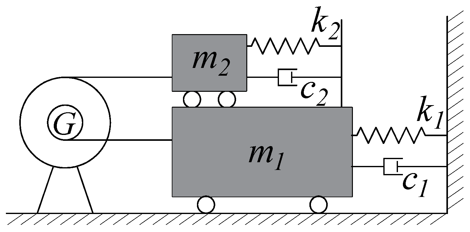
2.1. Topological Configuration of SAOD-LS

In this paper, a generalized SDOF system based on the fundamental configuration of the traditional AOD system is considered, as shown in Figure 1, where the mass m1 is the primary structure, and the mass m2 is the secondary mass. Please note that in this article, the symbols m1 and m2 are used to indicate the primary and secondary mass, respectively. This convention is consistently followed throughout the entire paper. When using a secondary linear spring (LS) in this new configuration, we refer to it as the SAOD-LS.
One terminal of k1 and c1 is linked to m1, while the other terminal is connected to the ground. One terminal of k2 and c2 is linked to m1, while the other terminal is linked to m2. The transmission device is connected to the ground, with a large radius attached to one end of m1 and a small radius connected to one end of m2. The transmission ratio, denoted as r, is defined as the ratio of the big radius to the small radius. It is important to mention that, based on the connection method of the transmission device shown in Figure 1, the movement directions of m1 and m2 are in opposing directions. The transmission device G, composed of a securely grounded rack-and-pinion system, serves to transform the linear motion of the rack into rotary motion for the pinion. By varying the radii of the pinions, the relative displacement between the input and output terminals can be adjusted by a factor of r (i.e., the gear ratio of G) [40]. As a result, m1 can transmit the amplified displacement, velocity, and acceleration to m2 through this device. Additionally, k2 and c2 contribute to the system’s functionality by absorbing and dissipating energy. According to the principle of conservation of energy, the energy gained by the secondary structure directly correlates to the energy lost by the building [39]. This interaction helps to reduce the oscillation amplitude of m1.

2.2. Derivation and Analytical Solution of the Motion Equation for SAOD-LS

Under the assumption that the system is not impacted by friction and the transmission is idealized with no energy dissipation [39], we can establish a generalized coordinate system by setting the equilibrium positions of m1 and m2 as the reference points. We mathematically formulate the total kinetic energy T and elastic potential energy V of the SAOD-LS, respectively.
T = 1 2 m 1 x ˙ 1 2 + 1 2 m 2 x ˙ 2 2
V = 1 2 k 1 x 1 2 + 1 2 k 2 x k 2 2
In Equations (1) and (2), the symbols x 1 and x ˙ 1 indicate the displacement and velocity of m1, respectively. The symbol x ˙ 2 represents the velocity of m2, while x k 2 represents the relative displacement between the two terminals of k2. Please note that in this article, the symbols x1 and x2 are used to indicate the primary and secondary mass displacement, respectively. This convention is consistently followed throughout the entire paper. Given a linear damping force, we can express the Rayleigh dissipation function (D) as follows:
D = 1 2 c 1 x ˙ 1 2 + 1 2 c 2 x ˙ c 2 2
In Equation (3), the symbol x ˙ c 2 represents the relative velocity between the two terminals of c2. Because the displacement of the link-secondary-structure end is r times that of the link-primary-structure end, the idealized relationship meets the following equation:
x 2 = r x 1 x ˙ 2 = r x ˙ 1 x ¨ 2 = r x ¨ 1
Due to the extremely small mass ratio (i.e., m2/m1) in actual bridges, as mentioned in [39], this study assumes that the forcing function acts only on the primary structure. By combining Equations (1)–(4) with the Lagrange Dynamic [39], we can formulate the motion equation of SAOD-LS as follows:
( m 1 + m 2 r 2 ) x ¨ 1 + [ c 1 + c 2 ( r + 1 ) 2 ] x ˙ 1 + [ k 1 + k 2 ( r + 1 ) 2 ] x 1 = m 1 x ¨ g
where x ¨ g is he horizontal ground acceleration [41].
The analytical solution to Equation (5) can be derived from its equivalent equation form, Equation (6).
x ¨ 1 + c 1 + c 2 ( r + 1 ) 2 m 1 + m 2 r 2 x ˙ 1 + k 1 + k 2 ( r + 1 ) 2 m 1 + m 2 r 2 x 1 = m 1 x ¨ g m 1 + m 2 r 2
The structure as a whole can be regarded as a SDOF system, as the displacement and velocity of m1 and m2 are connected by the transmission device. Equation (6) represents a standard differential equation for a SDOF system. To simplify the expression, the constant term in Equation (6) is substituted as below:
M = m 1 + m 2 r 2 C = c 1 + c 2 ( r + 1 ) 2 K = k 1 + k 2 ( r + 1 ) 2
where M, K, and C represent the generalized mass, generalized spring coefficient, and generalized damping coefficient, respectively [39]. Assuming the external excitation function is harmonic oscillation, the x ¨ g acts upon the following proposed dynamic system:
x ¨ g = a · sin ( θ t )
where a and θ represent the amplitude and frequency of the input acceleration, respectively.
The analytical solution of Equation (6) can be expressed as follows [42]:
x 1 = x t + x s
where xt and xs denote transient response and steady-state response, respectively. The explicit formulas for xt and xs are presented as follows:
x t = [ P · cos ( ω D t ) + μ · sin ( ω D t ) ] · exp ( ξ ω t )
x s = R [ ( 1 β 2 ) sin ( θ t ) ( 2 ξ β ) cos ( θ t ) ]
The parameters utilized in Equations (10) and (11) are listed as follows:
ω = K / M
β = θ / ω
ξ = C / ω ( 2 M ω )
ω D = ω 1 ξ 2
R = m 1 a K [ 1 ( 1 β 2 ) 2 + ( 2 ξ β ) 2 ]
P = 2 R ξ β + x 1 0
f l o a d = θ / ( 2 π )
μ = [ v 1 0 + ξ ω x 1 0 + 2 ξ 2 ω β R θ R ( 1 β 2 ) ] / ω D
where x 1 ( 0 ) and v 1 ( 0 ) represent the initial displacement and velocity of mass m1, respectively; ω signifies the undamped natural circular frequencies of SAOD-LS; β denotes the frequency ratio; ξ stands for the damping ratios; ωD indicates the damped natural circular frequencies of SAOD-LS; and fload designates the natural frequency of the applied load.

2.3. Validation of SAOD-LS Motion Equation and Its Performance Comparison with AOD

To assess the correctness of the SAOD-LS equation of motion and to compare its damping effect with that of AOD, we utilize Example 1, whose parameters are listed in Table 1.
In Example 1, the theoretical displacement solution of m1, designated as x1-Case 1, is derived using Equation (9). To validate the motion equation of SAOD-LS, we utilize the FE approach, and the result is denoted as x1-Case 2. In this FE modeling, m1 and m2 are represented using mass elements; the connecting rod is represented using a link element. Regarding the modeling method and boundary conditions, the one terminal of k1 and c1 is connected to m1, while another terminal is connected to the ground. The transmission device is emulated by controlling the forced displacement relationship between m1 and m2. The one terminal of k2 and c2 is connected to m1, while another terminal is connected to m2. Additionally, the time-history displacement results of AOD, obtained through the FE method, are labeled as x1-Case 3. The parameters for Case 3 are detailed in Table 1, with the only distinction being that Case 3 employs the AOD structure instead of the SAOD-LS used in Case 1 and Case 2. The results are visually represented in Figure 2.
The maximum discrepancy between x1-Case 1 and x1-Case 2 is 0.143 mm. The consistency observed between Case 1 and Case 2 suggests that both the SAOD-LS motion equation and its analytical solution are accurate. Additionally, only in Case 1 and Case 2 of this paper, the peak displacement of m1 in SAOD-LS is noticeably smaller compared to that of AOD. Only by adjusting the AOD connection mode, without any modifications to the model parameters, can we achieve this reduction. Specifically, by comparing Equation (5) from this study with Equation (10) from [39], one can observe that the amplification factor for c2 in C of SAOD-LS has been enlarged from r2 to (r + 1)2, similarly to the augmentation of k2 in K.

3. Composition and Working Principle of the NSD

3.1. Components and Derivation of Constitutive Equation for NSD

The NSD is a nonlinear spring device that incorporates connecting rods and linear springs arranged in a diamond pattern. It is primarily composed of four connecting rods, four hinges (Hinge A−D), a hinge-linked spring (Spring A), a spring without a hinge-linked spring (Spring B), and a cradle. These rods, functioning as truss elements, are interconnected via the hinges. Spring A is connected to Hinge A and Hinge C at its two ends, while a cradle is positioned in the middle of Spring A to hold Spring B. In the NSD’s initial position, where no external forces are applied and there is no displacement at terminals A and B, the terminals of Spring B maintain a preset distance from Hinges B and D. A detailed visual representation of the NSD’s structure is depicted in Figure 3a.
The NSD operates similarly to a spring with changing stiffness, and we view it as an integrated unit. To delineate the relationship between the equivalent external force, denoted as F, and the tension (or compression) of the NSD, represented by z, we introduce the following parameters: kA signifies the stiffness of Spring A, while kB corresponds to the stiffness of Spring B. Additionally, l1 designates the length of the connecting rod, l2 denotes half of Spring B’s length, and l3 represents half the distance between Hinge B and Hinge D. Given the NSD’s symmetry, it is advisable to consider Terminal A as the stationary terminal and Terminal B as the mobile one. As a result, F and z represent the force and displacement at Terminal B, respectively. For detailed parameter specifications, please refer to Figure 3b.
In this paper, it is clearly stated that when the NSD is under tension (specifically, when Terminal A and Terminal B are moving apart), z assumes a positive value (z > 0); otherwise, it becomes negative (z < 0). The value of z can be categorized into two distinct stages: the first ranging from −2(l3l2) to 2(l1l3) and the second from (−2l3) to −2(l3l2). These two stages correspond to two distinct situations: the first represents the NSD not in contact with Spring B, while the second represents the NSD in contact with Spring B. The relationship between F and z can be determined by applying the mechanical equilibrium equation for Hinges C and D, which are successively aligned. Following is an explanation of this relationship:
F = 2 k A · z p · l 4 l 5 / l 5 2 l 3 l 2 z < 2 l 1 l 3 2 k A · z p · l 4 l 5 / l 5 + F B 2 l 3 z < 2 l 3 l 2
The parameters used in Equation (20) are detailed below:
l 4 = 2 l 1 2 l 3 2
z p = N + 0.5 · z
l 5 = 2 l 1 2 z p 2
F B = k B · z + 2 l 3 l 2

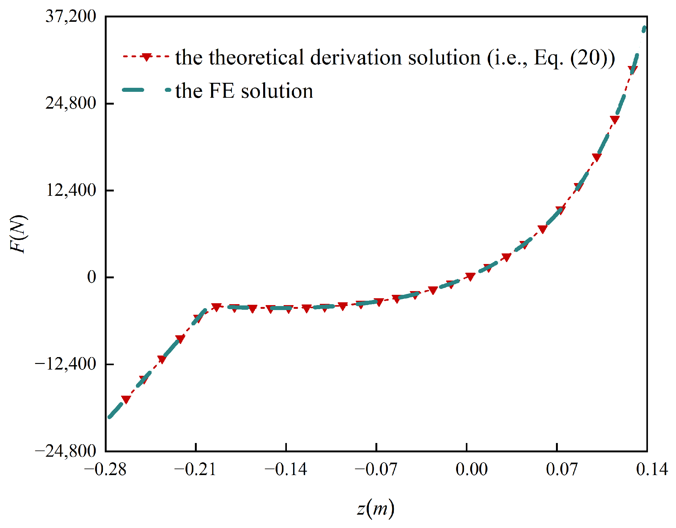
3.2. Verification of the Functional Relationship between F and z

To validate the accuracy of Equation (20), the NSD is evaluated using FE analysis. The parameters chosen for this simulation, specifically for Example 2, are as follows: The spring constant kA is set to 97 kN/m and kB to 221.8 kN/m, with lengths l1, l2, and l3 being 0.3 m, 0.1 m, and 0.2 m, respectively.
In the FE modeling process, initially, we make the assumption that the model is a two-dimensional planar model. The connecting rod is represented using a truss element, Spring A is modeled as a standard spring element, and Spring B is simulated as a nonlinear spring element. Given the NSD’s symmetry, it is advisable to consider Terminal A as the stationary terminal and Terminal B as the mobile one. So, assuming that all degrees of freedom of Terminal A are completely restricted. Terminal B undergoes forced displacement in the z-axis as illustrated in Figure 3b, and multi-step loading is facilitated by setting the number of displacement increments. By calculating the reactive force at Terminal B, we obtain the FE numerical solution for F. A comparison between the FE solution and the analytical data derived from Equation (20) is presented in Figure 4.
Figure 4 demonstrates the validity of Equation (20). Consistent with the analysis conducted using Equation (20), during compression of the device, F can be decomposed into two components: the component force from Spring A and the potential force from the highly stiff Spring B. During tension, while Spring B remains inactive, it becomes apparent that the change in angle of the connecting rods within the NSD leads to a notable increase in F.
In practical applications, the force and displacement of the required NSD should be calculated. Then, using Equation (20), the appropriate stiffness coefficient and stroke of Spring A and Spring B, as well as the connecting rod length, should be determined. Finally, the structure of the NSD will be ascertained. Materials have become more and more important in terms of high-strength spring steel [43], and a wide variety of high-strength spring steels are available to satisfy demand. For example, Chen et al. discovered that 55SiCrVNb had good yield strength and tensile strength after treatment [44].

4. Comparison of Shock Absorption Performance between SAOD-NSD and SAOD-LS

Figure 5 presents the mechanical model diagram of the SAOD-NSD, which is created by replacing the NSD with the constant value k2 of SAOD-LS. The only distinction between SAOD-NSD and SAOD-LS would be the secondary spring k2. In the SAOD-LS, k2 is an ideal spring with a certain stiffness coefficient, but in the SAOD-NSD, k2 refers to the NSD presented in Section 3.
To provide a clearer understanding of the exceptional damping abilities of the SAOD-NSD, we have selected Example 3 for illustration in this section. The parameters for the SAOD-LS and external excitation are set based on the values listed in Table 2.
By differentiating Equation (20) with respect to z, we can derive a function that describes the NSD’s equivalent stiffness, which corresponds to a specific z. This enables us to ascertain the equivalent stiffness for a particular set of geometric parameters (specifically, l1, l2, and l3) and spring constants (kA and kB). Referring to Example 3, Table 3 outlines the NSD parameters as mentioned. The NSD equivalent stiffness is calculated to be 1389.4 kN/m, which coincides with the SAOD-LS k2 in Table 3.
Using Table 2 and Equation (7), it can be determined that the natural frequency of SAOD-LS (fSAOD-LS) is 4.53 Hz. In Example 3, the value of fload falls within the range of 0.95 fSAOD-LS to 1.05 fSAOD-LS, which is classified as the near-resonance region according to reference [45].
The value x1max is defined as the peak value of the m1’s time-history displacement response to external excitation. Figure 6 compares the x1max curve between the SAOD-NSD and the SAOD-LS under 50 s harmonic loads at different frequencies (i.e., fload). In this instance, x1max is calculated by the FE method. During the FE modeling process, the NSD is integrated into a spring element that exhibits nonlinear behavior depicted in Equation (20). The other modeling methods remain consistent with those used in Example 1.
Figure 6 clearly illustrates that at the exact resonance point, the x1max of the SAOD-NSD is 22 mm, notably less than the 162 mm observed in the SAOD-LS. Throughout the entire near-resonance region, the x1max of the SAOD-NSD remains below 40% of that of SAOD-LS. This indicates that the NSD exhibits exceptional damping effectiveness in the near-resonance region.
Similar to many SDOF dampers, time-history analysis reveals a distinct resonance phenomenon when the parameters of the SAOD-LS and external stimulation remain constant. In addition, despite the SAOD-NSD demonstrating resonance-like characteristics, its resonance peak can be significantly reduced. This study utilizes Example 4, which involves three distinct cases [40].
Case 4 is the classic SDOF mass-spring-damper system, as depicted in Figure 1.6.1a in [46]. In Case 4, the mass (m1) is set at 29,485 kg, the spring constant (k1) at 3800 kN/m, and the damping coefficient (c1) at 3740 Ns/m. Please refer to Figure 7 for schematic sketches depicting Case 5 and Case 6. The main structural forms of Case 5 and Case 6 are exactly the same, except for the fact that k2 and k3 in Case 5 are LSs (i.e., linear springs), whereas in Case 6, they are NSDs (i.e., the nonlinear spring devices).
In Case 5, the values of k2 and k3 are set at 1389.4 kN/m. As for Case 6, the NSD parameters k2 and k3 are consistent with the values specified in Table 3. Additionally, the external excitation in Example 4 is represented by the formula x ¨ g = 38sin(2π·1.81t). For further details on the other parameters of both Case 5 and Case 6, please refer to Table 4.
The natural frequencies of Case 4 and Case 5 are both 1.81 Hz, thereby satisfying resonance. The main objective of Case 6’s structure design is to minimize the impact of the force change of NSD during both the tension and compression stages. The organization of Case 5 facilitates the comparison of Case 6. The NSD’s equivalent stiffness in Case 6 is identical to that of Case 5, making both cases comparable. Figure 8a displays the time-history displacements of m1 in Case 4, Case 5, and Case 6, specifically for the first 12 s. The FE technique is used to calculate the results. We use NSD for a nonlinear-spring element. The following modeling steps are identical to those in Example 1.
Figure 8a demonstrates that in Case 5, the SAOD-LS exhibits a notable damping effect at resonance, resulting in a reduction in the displacement peak at resonance. In comparison, the peak resonance of the SAOD-NSD in Case 6 appears lower. Meanwhile, the time-history response indicates that the SAOD-NSD exhibits a resonance-like phenomenon, but with a significant reduction in its response peak.
Subsequently, aiming to facilitate a more in-depth investigation of the damping mechanism of the NSD in comparison to LS, the amplitude spectrum is employed for analyzing both the frequency components and the amplitude of the response. The m1 displacement responses of Case 4, Case 5, and Case 6 during the first 300 s are subjected to Fourier transformation. We analyze the amplitude spectra of the filtered data and present the results in Figure 8b.
Upon examination of Figure 8b, it is evident that the frequency of 1.81 Hz corresponds to both the natural frequency of the structure and the frequency of external excitation in Case 4 and Case 5. Notably, the peak value at Point B (Case 5) is considerably lower than that at Point A (Case 4), corroborating the results obtained through time-history analysis.
Given that the equivalent stiffness of the NSD in Case 6 is equal to the stiffness of the LS in Case 5, it can be inferred that the frequency at Point D in Case 6 is also 1.81 Hz. Additionally, the NSD contributes to Point C, which displays a greater amplitude than Point D. When comparing Case 5 and Case 6, it becomes evident that the NSD not only consumes low-frequency energy but also demonstrates remarkable energy dissipation capacity.
To gain a deeper understanding of how amplitude spectra evolve over time, the evolutionary power spectral density (EPSD) method has been adopted. Since both Case 4 and Case 5 in Example 4 are SDOF structures, their EPSD results exhibit substantial similarity. Therefore, there is no need to analyze them separately in this context. Consequently, we have generated a graph illustrating the EPSD outcome specifically for Case 6 over the initial 420 s, as depicted in Figure 9.
By investigating Figure 8b and Figure 9 together, it becomes evident that the highest energy consumption at Point C, caused by NSD in Figure 8b, is more effective than that at Point D at the beginning. However, the peak energy consumption at Point C decreases over time. Nonetheless, in practical seismic problems, the displacement peak typically occurs during the initial several minutes of vibration, known as the transient term. Therefore, the practical application of the NSD to vibration concerns remains valuable.
In summary, the SAOD-LS demonstrates a significant capacity to reduce the peak amplitude of the response. As for the SAOD-NSD, although the NSD cannot fully eliminate the resonance effect, it still manages to notably diminish the maximum amplitude of the response.

5. Damping Performance of SAOD-LS and SAOD-NSD in an Actual Bridge Example

To illustrate the profound effect of the SAOD-LS and SAOD-NSD in mitigating vibrations of real bridge structures, this section employs a six-span continuous beam bridge from the Puwan 14th Bridge located in the Puwan New Area of Dalian as Example 5. This bridge is a twin-deck concrete continuous beam bridge that plays a vital role in Puwan New Area’s transportation network.
As shown in Figure 10, Example 5 has a span arrangement of 70 m + 120 m + 120 m + 120 m + 70 m, summing up to a total length of 500 m. The piles, piers, and main girder were constructed using concrete grades C30, C40, and C50, respectively. The seismic fortification intensity for Dalian stands at 8 degrees, with a corresponding design seismic acceleration peak value of 0.2 g [47,48,49].
The El Centro wave, scaled to a magnitude of 2.1 times, was selected as the external excitation for our analysis. We conducted a comparative study on the displacement of the main girder in three different cases: the original bridge (labeled as Case 7), the bridge equipped with two identical SAOD-LS devices on both abutments (Case 8), and the bridge equipped with two identical SAOD-NSD devices on both abutments (Case 9). Regarding the SAOD-LS and SAOD-NSD, it can be considered that the main beam of the bridge is the primary structure, while the transmission device can be positioned on the abutment. Additionally, the secondary structure can be located within the bridge’s box-girder. This arrangement effectively addresses the challenge of installing the secondary structure of the AOD. The specific parameters chosen for the SAOD-NSD devices in Case 9 on one side of the abutment are presented in Table 5.
Apart from the k2 of the SAOD-LS in Case 8, which is precisely set to 100 kN/m, all the other parameters for the SAOD-LS in Case 8 are identical to those in Case 9 (i.e., m2 = 180 t, c2 = 0 Ns/m and r2 = 5). We compute the displacement and force results in Section 5 using the FE method. The general FE modeling method (i.e., the finite element analysis) for beam bridges models the Puwan 14th Bridge part. The modeling methods for the SAOD-LS and SAOD-NSD are similar to Example 4, with the distinction that the main girder of the bridge is treated as the primary structure, including m1, c1, and k1. Figure 11 illustrates a comparison of the main girder’s time-history displacement response during the first 10 s for Case 7, Case 8, and Case 9.
After researching Figure 11, it is observed that within the first 10 s, the maximum value for x1-Case 7 reaches 17.93 cm, while x1-Case 8 is 13.55 cm (reflecting a seismic reduction rate of 24.43%), and x1-Case 9 is 13.15 cm (showing a seismic reduction rate of 26.66%). This suggests that both SAOD-LS and SAOD-NSD exhibit exceptional shock absorption capabilities for the actual bridge.
Note: seismic reduction rate = (maximum structural response without control − maximum structural response with control)/maximum structural response without control [50].
A vibration reduction system with remarkable robustness implies that, under different types of seismic waves, the system demonstrates superior damping performance. Therefore, in the following study, we selected three near-field and three far-field seismic waves [51,52,53,54], listed in Table 6.
We calculate the seismic reduction rate for the main girder displacement and the bending moment at the bottom of the middle pier equipped with the SAOD-LS and SAOD-NSD, respectively. Figure 12 illustrates that the SAOD-LS and SAOD-NSD exhibit effective damping properties against various types of seismic waves, indicating their outstanding robustness as damping devices.

6. Concluding Remarks

In order to solve the problem of the secondary system arrangement and improve the damping efficiency of the AOD with equivalent values of parameters (i.e., Improvement needed 1 mentioned in Introduction), this paper introduces the SAOD-LS, in which the secondary spring and damper are connected to the primary structure. We derive the SAOD-LS system’s motion equation from the Lagrange Dynamic and verify it using the FE approach. The SAOD-LS demonstrates a significant capacity to reduce the peak amplitude of the response. Considering that in practical applications, r can reach about 10, raising r will further improve the damping performance [40]. As a result, the SAOD-LS offers a wide range of useful applications. SAOD-LS’s rapid response to providing the damping effect is a significant mechanical characteristic that is strongly tied to its unique nature as a SDOF damper. Future anti-ice collisions on piers may utilize this mechanical characteristic.
Additionally, an innovative nonlinear spring device (NSD) was proposed, wherein connecting rods and linear springs are arranged in a diamond pattern. Its constitutive relationship can be expressed as a piecewise function, which is checked by the FE analysis. In summary, the device exhibits the following mechanical characteristics: when the relative displacement between the NSD’s two terminals is small, the force (F) is also small; however, if the relative displacement between the NSD’s two terminals is large, the device will generate a considerably large force (F). The device lays the groundwork for future applications in fields such as civil engineering and machinery. For instance, in the context of controlling displacement and force along the longitudinal direction of the bridge, it enables the controlled release of small displacements caused by temperature changes and regular vehicle loads. However, in the event of abnormal excitations, such as earthquakes, the device exerts significant force to prevent excessive displacement of the main girder.
Also, in order to realize the Improvement needed 2, mentioned in Introduction, the SAOD-NSD, which is an SDOF system made by combining the NSD and SAOD-LS, has a much better damping effect in the near-resonance area than the SAOD-LS. At exact resonance, the SAOD-NSD exhibits a resonance-like phenomenon, but the peak value of the response is much smaller. When the characteristic frequency of an earthquake closely matches the natural frequency of the structure, the utilization of NSD for shock absorption becomes highly significant. It is noteworthy that while Case 3 in Example 4 fully utilizes the nonlinear stage of the NSD, it also stays within the maximal applicability range of the NSD. In future research, on the one hand, it is crucial to ensure a sufficient safety margin for NSDs to prevent damage from excessive force. On the other hand, it is critical that we make great efforts to ensure that NSD’s strong nonlinear stage plays an active role in the task. Otherwise, the NSD cannot fully utilize its distinctive features.
Last but not least, this research applies the SAOD-LS and SAOD-NSD to an actual bridge project, demonstrating that both devices effectively absorb shocks in practical applications. By analyzing the response to various seismic waves, it is evident that both devices exhibit strong robustness.
It is noteworthy that the SAOD-LS and SAOD-NSD also have certain restrictions on their applications. With the SAOD-LS as an example, engineers ought to calculate the values of M, C, and K in the Equation (7) for practical use while designing the device. Practical engineering generally establishes m1, k1, and c1, so the focus should solely be on determining the values of m 2 r 2 , k 2 ( r + 1 ) 2 , and c 2 ( r + 1 ) 2 . The approach presented in this study attempts to determine the values of m2, k2, and c2 under the condition of a constant r. Determining the values of m2, k2, and c2 first, and then figuring out r’s value, is particularly easily accessible for engineering practice. In subsequent investigation, it appears that this issue can be resolved by adjusting the values of rm2, rk2, and rc2, (i.e., different r for m2, k2, and c2).
This study has also laid the groundwork for future research. Simultaneously, it is hoped that this study will lead to new insights into bridge earthquake resistance.

Author Contributions

Conceptualization, Y.T., M.S. and Z.L.; methodology, Q.Z., Y.T. and M.S.; software, Q.Z., M.S. and Y.J.; validation, P.W.; formal analysis, Q.Z., M.S. and Y.J.; investigation, F.M.; resources, Y.T. and Z.L.; data curation, M.S.; writing—original draft preparation, Q.Z., Y.J. and F.M.; writing—review and editing, Y.T. and Z.L.; visualization, M.S. and F.M.; supervision, Y.T., M.S. and Z.L.; project administration, Z.L.; funding acquisition, Z.L. All authors have read and agreed to the published version of the manuscript.

Funding

This work was supported by the project from National Natural Science Foundation of China (the grant number U23A2012).

Data Availability Statement

The original contributions presented in the study are included in the article, for a more detailed data request, please contact the corresponding author directly.

Conflicts of Interest

Author Minggang Sun was employed by the company Longjian Road and Bridge Company Limited. The remaining authors declare that the research was conducted in the absence of any commercial or financial relationships that could be construed as a potential conflict of interest.

References

  1. Tabatabai, S.M.; Tabatabai, F.A.-S. Integrating Inverse Data Envelopment Analysis and Machine Learning for Enhanced Road Transport Safety in Iran. J. Soft Comput. Civ. Eng. 2024, 8, 141–160. [Google Scholar] [CrossRef]
  2. Zhang, G.; Liu, Y.; Liu, J.; Lan, S.; Yang, J. Causes and Statistical Characteristics of Bridge Failures: A Review. J. Traffic Transp. Eng. 2022, 9, 388–406. [Google Scholar] [CrossRef]
  3. Kronprasert, N.; Boontan, K.; Kanha, P. Crash Prediction Models for Horizontal Curve Segments on Two-Lane Rural Roads in Thailand. Sustainability 2021, 13, 9011. [Google Scholar] [CrossRef]
  4. Morfidis, K.; Kostinakis, K. Rapid Prediction of Seismic Incident Angle’s Influence on the Damage Level of RC Buildings Using Artificial Neural Networks. Appl. Sci. 2022, 12, 1055. [Google Scholar] [CrossRef]
  5. Morfidis, K.; Stefanidou, S.; Markogiannaki, O. A Rapid Seismic Damage Assessment (RASDA) Tool for RC Buildings Based on an Artificial Intelligence Algorithm. Appl. Sci. 2023, 13, 5100. [Google Scholar] [CrossRef]
  6. Kostinakis, K.; Morfidis, K.; Demertzis, K.; Iliadis, L. Classification of Buildings’ Potential for Seismic Damage Using a Machine Learning Model with Auto Hyperparameter Tuning. Eng. Struct. 2023, 290, 116359. [Google Scholar] [CrossRef]
  7. Konar, T. Seismic Vibration Control of a Building by Overhead Water Tank Designed as Slender Tuned Sloshing Damper. Pract. Period. Struct. Des. Constr. 2024, 29, 04023069. [Google Scholar] [CrossRef]
  8. Zhang, J.; Wu, B. Research on Smart Control Tests of Ice-induced Vibration Control of Offshore Platform. In Proceedings of the 2010 International Conference on Intelligent Control and Information Processing, Dalian, China, 13–15 August 2010; pp. 342–347. [Google Scholar] [CrossRef]
  9. Sun, Z.; Zou, Z.; Ying, X.; Li, X. Tuned Mass Dampers for Wind-induced Vibration Control of Chongqi Bridge. J. Bridge Eng. 2020, 25, 05019014. [Google Scholar] [CrossRef]
  10. Hawryszków, P.; Pimentel, R.; Silva, R.; Silva, F. Vertical Vibrations of Footbridges Due to Group Loading: Effect of Pedestrian–Structure Interaction. Appl. Sci. 2021, 11, 1355. [Google Scholar] [CrossRef]
  11. Bedon, C.; Santos, F.A. Effect of Spring-Mass-Damper Pedestrian Models on the Performance of Low-Frequency or Lightweight Glazed Floors. Appl. Sci. 2023, 13, 4023. [Google Scholar] [CrossRef]
  12. Huang, Z.; Shi, X.; Mu, D.; Huang, X.; Tong, W. Performance and Optimization of a Dual-Stage Vibration Isolation System Using Bio-Inspired Vibration Isolators. Appl. Sci. 2022, 12, 11387. [Google Scholar] [CrossRef]
  13. He, H.; Tan, P.; Hao, L. Acceleration-based Effective Damping Ratio of Tuned Mass Damper under Seismic Excitations. Struct. Des. Tall Spec. 2022, 31, e1910. [Google Scholar] [CrossRef]
  14. Kiani, M.; Enayati, H. Evaluation of a Nonlinear TMD Seismic Performance for Multi-degree of Freedom Structures. Asian J. Civil Eng. 2018, 25, 1395–1412. [Google Scholar] [CrossRef]
  15. Bousouar, A.; Harzallah, S.; Nail, B.; Tibermacine, I.E. An Investigation on the Effects of Using TMD for Vibration Control on the Response of High-rise Buildings to Seismic Excitation. Stud. Eng. Exact Sci. 2024, 5, 2–18. [Google Scholar] [CrossRef]
  16. Wang, M.; Nagarajaiah, S.; Chen, L. Adaptive Passive Negative Stiffness and Damping for Retrofit of Existing Tall Buildings with Tuned Mass Damper: TMD-NSD. J. Struct. Eng. 2022, 148, 04022180. [Google Scholar] [CrossRef]
  17. Frahm, H. Device for Damping Vibrations of Bodies. U.S. Patent 9,899,58A, 18 April 1911. [Google Scholar]
  18. Fujino, Y.; Abé, M. Design Formulas for Tuned Mass Dampers Based on a Perturbation Technique. Earthq. Eng. Struct. Dyn. 1993, 22, 833–854. [Google Scholar] [CrossRef]
  19. Fujino, Y. Vibration, Control and Monitoring of Long-span Bridges—Recent Research, Developments and Practice in Japan. J. Constr. Steel Res. 2002, 58, 71–97. [Google Scholar] [CrossRef]
  20. Fujino, Y.; Yoshida, Y. Wind-induced Vibration and Control of Trans-Tokyo Bay Crossing Bridge. J. Struct. Eng. 2002, 128, 1012–1025. [Google Scholar] [CrossRef]
  21. Mazzon, L.; Frappa, G.; Pauletta, M. Effectiveness of Tuned Mass Damper in Reducing Damage Caused by Strong Earthquake in a Medium-Rise Building. Appl. Sci. 2023, 13, 6815. [Google Scholar] [CrossRef]
  22. Pellizzari, F.; Marano, G.; Palmeri, A.; Greco, R.; Domaneschi, M. Robust Optimization of MTMD Systems for the Control of Vibrations. Probabilistic Eng. Mech. 2022, 70, 103347. [Google Scholar] [CrossRef]
  23. Wang, Z.; Zhou, L.; Chen, G. Optimal Design and Application of a MTMD System for a Glulam Footbridge under Human-induced Excitation. Eur. J. Wood Wood Prod. 2022, 81, 529–545. [Google Scholar] [CrossRef]
  24. Xu, K.; Igusa, T. Dynamic Characteristics of Multiple Substructures with Closely Spaced Frequencies. Earthq. Eng. Struct. Dyn. 1992, 21, 1059–1070. [Google Scholar] [CrossRef]
  25. Wielgos, P.; Geryło, R. Optimization of Multiple Tuned Mass Damper (MTMD) Parameters for a Primary System Reduced to a Single Degree of Freedom (SDOF) through the Modal Approach. Appl. Sci. 2021, 11, 1389. [Google Scholar] [CrossRef]
  26. Smith, M.C. Synthesis of Mechanical Networks: The Inerter. IEEE Trans. Autom. Control 2002, 47, 1648–1662. [Google Scholar] [CrossRef]
  27. Ikago, K.; Saito, K.; Inoue, N. Seismic Control of Single-degree-of-freedom Structure Using Tuned Viscous Mass Damper. Earthq. Eng. Struct. Dyn. 2012, 41, 453–474. [Google Scholar] [CrossRef]
  28. Kawamata, S. Development of a Vibration Control System of Structures by Means of Mass Pump; Institute of Industrial Science, University of Tokyo: Tokyo, Japan, 1973. [Google Scholar]
  29. Kawamata, S.; Funaki, N.; Itoh, Y. Passive Control of Building Frames by Means of Liquid Dampers Sealed by Viscoelastic Material. In Proceedings of the 12th World Conference on Earthquake Engineering, Auckland, New Zealand, 1–4 February 2000. [Google Scholar]
  30. Saito, K.; Toyota, K.; Nagae, K.; Sugimura, Y.; Nakano, T.; Nakaminam, I.S.; Arima, F. Dynamic Loading Test and Application to a High-rise Building of Viscous Damping Devices with Amplification System. In Proceedings of the Third World Conference on Structural Control, Como, Italy, 11 April 2002. [Google Scholar]
  31. Saito, K.; Sugimura, Y.; Nakaminami, S.; Kida, H.; Inoue, N. Vibration Tests of 1-story Response Control System Using Inertial Mass and Optimized Soft Spring and Viscous Element. In Proceedings of the 14th World Conference on Earthquake Engineering, Beijing, China, 12–17 November 2008. [Google Scholar]
  32. Ikago, K.; Sugimura, Y.; Saito, K.; Inoue, N. Optimum Seismic Response Control of Multiple Degree of Freedom Structures Using Tuned Viscous Mass Dampers. In Proceedings of the Tenth International Conference on Computational Structures Technology, Valencia, Spain, 14–17 September 2010. [Google Scholar]
  33. Zhang, R.; Wu, M.; Ren, X.; Pan, C. Seismic Response Reduction of Elastoplastic Structures with Inerter Systems. Eng. Struct. 2021, 230, 111661. [Google Scholar] [CrossRef]
  34. Chen, M.; Papageorgiou, C.; Scheibe, F.; Wang, F.; Smith, M. The Missing Mechanical Circuit Element. IEEE Circuits Syst. Mag. 2009, 9, 10–26. [Google Scholar] [CrossRef]
  35. Papageorgiou, C.; Houghton, N.E.; Smith, M.C. Experimental Testing and Analysis of Inerter Devices. J. Dyn. Syst. Meas. Control 2009, 131, 101–116. [Google Scholar] [CrossRef]
  36. Liu, X.; Yang, Y.; Sun, Y.; Zhong, Y.; Zhou, L.; Li, S.; Wu, C. Tuned-Mass-Damper-Inerter Performance Evaluation and Optimal Design for Transmission Line under Harmonic Excitation. Buildings 2022, 12, 435. [Google Scholar] [CrossRef]
  37. Shen, W.; Niyitangamahoro, A.; Feng, Z.; Zhu, H. Tuned Inerter Dampers for Civil Structures Subjected to Earthquake Ground Motions: Optimum Design and Seismic Performance. Eng. Struct. 2019, 198, 109470. [Google Scholar] [CrossRef]
  38. Li, C.; Zhang, L. Evaluation of the Dual-layer Multiple Tuned Mass Dampers for Structures Subjected to Earthquake. J. Vib. Shock 2005, 24, 45–46+134. (In Chinese) [Google Scholar] [CrossRef]
  39. Tan, Y.; Guan, R.; Zhang, Z. Performance of Accelerated Oscillator Dampers under Seismic Loading. Adv. Mech. Eng. 2018, 10, 2072045839. [Google Scholar] [CrossRef]
  40. Zhou, J. Damping Performance and Optimization of Accelerated Oscillator Dampers. Master’s Thesis, Dalian University of Technology, Dalian, China, 2019. (In Chinese) [Google Scholar] [CrossRef]
  41. Tan, Y.; Chen, T.; Li, Z. Performance of Optimum Accelerated Oscillator Damper-based Isolation System for Buildings. Eng. Struct. 2021, 235, 112044. [Google Scholar] [CrossRef]
  42. Clough, R.W.; Penzien, J. Dynamics of Structures; Computer and Structures: Berkeley, CA, USA, 2003. [Google Scholar]
  43. Wang, X. Development Status and Trend Analysis of High Strength Spring Steel. China’s Manganese Ind. 2017, 35, 104–106. (In Chinese) [Google Scholar] [CrossRef]
  44. Chen, K.; Jiang, Z.; Liu, F.; Yu, J.; Li, Y.; Gong, W.; Chen, C. Effect of Quenching and Tempering Temperature on Microstructure and Tensile Properties of Microalloyed Ultra-high Strength Suspension Spring Steel. Mat. Sci. Eng. A Struct. 2019, 766, 138272. [Google Scholar] [CrossRef]
  45. Lu, Y.; Wu, X.; Zhu, L.; Cao, L. Application of 3σ Theorem in the Partition of Resonance Zone. J. Mach. Des. 2008, 25, 48–50. (In Chinese) [Google Scholar] [CrossRef]
  46. Chopra, A.K. Dynamics of Structures, Theory and Applications to Earthquake Engineering, 4th ed.; Pearson Education Limited: Upper Saddle River, NJ, USA, 2013. [Google Scholar]
  47. GB 50011-2010; Code for Seismic Design of Buildings. Architecture and Industry Press: Beijing, China, 2016.
  48. Dong, S.; Zhang, X.; Jia, C.; Li, S.; Wang, K. Study on Seismic Response and Vibration Reduction of Shield Tunnel Lining in Coastal Areas. Sustainability 2023, 15, 4185. [Google Scholar] [CrossRef]
  49. Chang, J.; Deng, Y.; Mu, H. Effects of the Earth Fissure on the Seismic Response Characteristics of Nearby Metro Stations and Tunnels. B Eng. Geol. Environ. 2023, 82, 232. [Google Scholar] [CrossRef]
  50. Li, H.; Yin, Y.; Wang, S. Studies on Seismic Reduction of Story-increased Buildings with Friction Layer and Energy Dissipated Devices. Earthq. Eng. Struct. Dyn. 2003, 32, 2143–2160. [Google Scholar] [CrossRef]
  51. Sarvestani, H.A. Structural Evaluation of Steel Self-centering Moment-resisting Frames under Far-filed and Near-field Earthquakes. J. Constr. Steel Res. 2018, 151, 83–93. [Google Scholar] [CrossRef]
  52. Gorai, S.; Maity, D. Seismic Response of Concrete Gravity Dams under Near Field and Far Field Ground Motions. Eng. Struct. 2019, 196, 109292. [Google Scholar] [CrossRef]
  53. Li, Y.; Tian, Y.; Zong, J. Seismic Responses of a Tunnel-soil-surface Structure System under Multidimensional Near-field and Far-field Seismic Waves through a Shaking Table Test. KSCE J. Civ. Eng. 2022, 26, 4717–4736. [Google Scholar] [CrossRef]
  54. Etedali, S.; Akbari, M.; Seifi, M. MOCS-based Optimum Design of TMD and FTMD for Tall Buildings under Near-field Earthquakes including SSI Effects. Soil Dyn. Earthq. Eng. 2019, 119, 36–50. [Google Scholar] [CrossRef]
Figure 1. Schematic diagram of SAOD-LS.
Applsci 14 06732 g001
Figure 2. Time-history displacement response x1.
Applsci 14 06732 g002
Figure 3. The NSD’s diagram of (a) structural form, (b) geometric parameters.
Applsci 14 06732 g003
Figure 4. The relationship between the equivalent external force, F, and the tension (or compression) of NSD, z, obtained through FE simulations and theoretical derivations.
Applsci 14 06732 g004
Figure 5. Schematic diagram of SAOD-NSD.
Applsci 14 06732 g005
Figure 6. x1max comparison of SAOD-NSD and SAOD-LS. In this modeling, the exact resonance frequency (4.53 Hz) is shown by the red dash line, and the values of SAOD-NSD and SAOD-LS’s x1max at exact resonance are represented by the symbol Applsci 14 06732 i001.
Applsci 14 06732 g006
Figure 7. Schematic diagram of Case 5 or Case 6.
Applsci 14 06732 g007
Figure 8. Example 4 result comparison: (a) time-history displacement response of m1. Applsci 14 06732 i001 
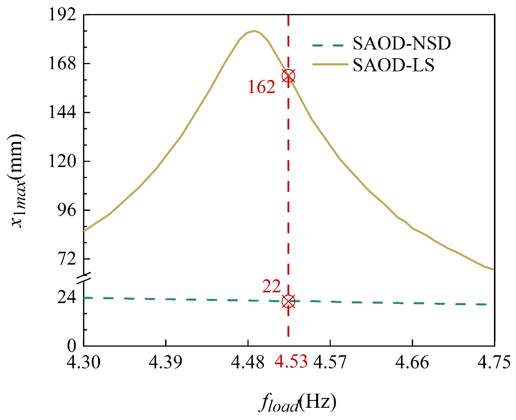
reflects the x1max (i.e., the maximum time-history displacement of primary mass m1) within the initial 12 s of this case; (b) amplitude spectrum result.
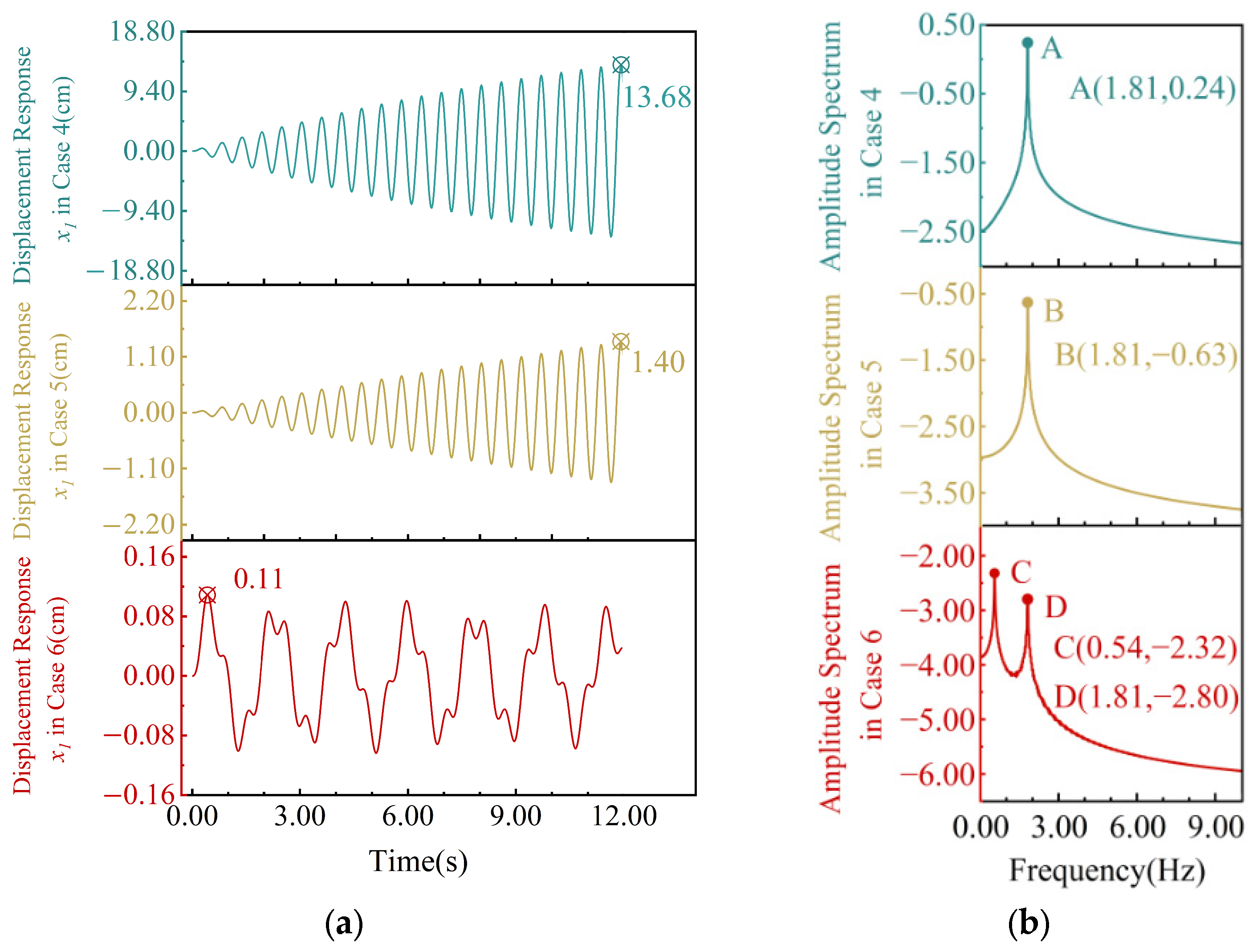
Applsci 14 06732 g008
Figure 9. Amplitude spectrum in Case 4, Case 5 and Case 6.
Applsci 14 06732 g009
Figure 10. General layout of half of Example 5 (units: m).
Applsci 14 06732 g010
Figure 11. Comparison of the main girder’s time-history displacement response for Case 7, Case 8, and Case 9.
Applsci 14 06732 g011
Figure 12. Seismic reduction rate of (a) the main girder displacement; (b) the middle-pier-bottom bending moment.
Applsci 14 06732 g012
Table 1. Values of parameters in Example 1.
m1 (kg)m2 (kg)k1 (N/m)k2 (N/m)c1 (Ns/m)c2 (Ns/m)x1 (0) (m)v1 (0) (m/s)fload (Hz)a (m/s2)r
100040100,000400010040001.27−3.84
Table 2. Values of parameters in Example 3.
m1 (kg)m2 (kg)k1 (kN/m)k2 (kN/m)c1 (Ns/m)c2 (Ns/m)x1 (0) (m)v1 (0) (m/s)a (m/s2)r
29,48530038001389.4374023700−53
Table 3. Values of NSD parameters in Example 3 and Case 6 of Example 4.
kA (kN/m)kB (kN/m)l1 (m)l2 (m)l3 (m)
47.252425.850.800.350.40
Table 4. Values of other parameters of Case 5 and Case 6 in Example 4.
m1 (kg)m2 (kg)m3 (kg)k1 (kN/m)c1 (Ns/m)c2 (Ns/m)c3 (Ns/m)r2r3
29,48519,16519,1653800374023723733
Table 5. Values of one-side-abutment parameters of Case 9 in Example 5.
m2 (t)c2 (Ns/m)r2kA (kN/m)kB (kN/m)l1 (m)l2 (m)l3 (m)
1800581.3081.300.730.380.40
Table 6. The seismic waves selected in Example 5.
TypeSeismic Wave NumberSeismic Wave Name
Far-field1El Centro
2Chi Chi, Chiayi Taiwan China #CHY086
3Loma Prieta, Hayward—Bart Sta.
Near-field4Landers
5Northridge
6Kobe
Disclaimer/Publisher’s Note: The statements, opinions and data contained in all publications are solely those of the individual author(s) and contributor(s) and not of MDPI and/or the editor(s). MDPI and/or the editor(s) disclaim responsibility for any injury to people or property resulting from any ideas, methods, instructions or products referred to in the content.

