Structural Design and Analysis of Multi-Directional Foot Mobile Robot

Abstract

Traditional mobile robots have limited mobility in complex terrain environments. Generally, the closed-chain leg structure of a foot-type robot relies on the speed difference to turn, but it is difficult to complete the turning action in narrow spaces. Therefore, this study proposes a closed-chain foot-type robot that can move in multiple directions, inspired by the WATT-I leg structure. Firstly, the closed-chain single-leg structure is designed, and the leg structure is analyzed in terms of the degrees of freedom, kinematics, and singularity. A simulation is also carried out. Secondly, based on the present trajectory, a heuristic algorithm is used to solve the inverse trajectory problem, and the size of the mechanism is optimized. Finally, the steering mechanism of the leg with a zero turning radius is designed and analyzed, which achieves the steering function of the whole robot and satisfies the goal of enabling the foot robot to walk in all directions. This study provides theoretical guidance for the structural dimension optimization of the proposed foot mobile robot and its application in engineering fields such as rescue, exploration, and the military.

1. Introduction

With the increasing labor costs, the rising shortage of human resources, and the limitations of the working environment, robots with high efficiency, low costs, and strong environmental adaptability have attracted much attention. Traditional wheeled and tracked robots have limited mobility in complex and irregular terrain environments [1,2,3,4,5]. In this context, research on foot robots is booming. In the face of rugged, rocky, sandy, steep, and complex terrain, mobile foot robots can meet the corresponding requirements, and their environmental adaptability is very strong [6,7,8,9,10] in the process of movement. The main feature of the parallel robot in terms of its structure is the closed-chain constraint. Compared with the open-chain leg structure, the closed-chain leg structure has higher strength and rigidity, accurate control, and a single-power drive, but it also reduces its flexibility. Generally speaking, a foot robot with a closed-chain leg structure relies on the speed difference between the two feet to turn. There is a certain turning space requirement for a footed robot, and it is difficult to complete the turning action in narrow spaces. Therefore, the design of a closed-chain footed robot that can move laterally has certain application value.

The walking systems of foot robots has always been a research hotspot in the field of robots at home and abroad [11,12,13]. The walking mechanism is the core element that enables footed robots to maintain their walking stability, passing efficiency, and working reliability in complex unstructured environments. The legs of existing foot robots involve mainly open kinematic chains, which are composed of legs, feet, and connecting rods in series, and the motor drives the joints to reciprocate; the open chain leg mechanism has the advantages of a simple structure, a large working space, and flexible walking. However, this structural form also has the following limitations: the leg structure has low rigidity and is not suitable for large-capacity tasks; from the perspective of quality, control difficulties, and development costs, it is a great challenge to arrange the open kinematic chain as a whole multi-legged form.

In comparison, mechanical legs based on a closed kinematic chain involve mostly single-degree-of-freedom linkage mechanisms, which use the full-circle rotation drive of the crank to achieve a single-leg swing walking output. The coordinated configuration of the mechanical phases replaces the synchronous control of multiple motors; it is suitable for the multi-foot layout of the whole machine and enables better load-bearing performance and overall rigidity. With the continuous research and development of closed-chain leg mechanisms, there are many types of such mechanisms used in mechanical legs, including the three classic closed-chain leg mechanisms consisting of the Chebyshev mechanism [14,15], Jansen mechanism [16,17,18], and Klann mechanism [19,20,21]. Researchers at home and abroad have used the Chebyshev four-bar mechanism to construct a zoom-type closed-chain leg mechanism by combining it with a magnifying mechanism [22,23,24,25,26]. At the same time, Chinese scholars have also conducted extensive research and exploration on the planar closed-chain single-leg configuration [27,28,29,30,31,32]. Wang created a restoration design for the “Wooden Cow and Flowing Horse” in the Three Kingdoms period and proposed a single-leg eight-bar linkage mechanism that places the four-legged mechanical horse behind two passive wheels to form a wooden carriage.

The closed-chain leg mechanism system resolves the control complexity of the series system. It adopts the structural form of multi-link coupling, which enables good overall stiffness and simplifies the motion control system. In order to avoid the energy consumption caused by the inertia of the leg mechanism when the linear actuator is reversed, the whole rotation drive is used, instead of a reciprocating drive, which is conducive to the improvement of the moving efficiency and step frequency. Therefore, differing from the open-chain leg mechanism, this study designs a closed-chain single-leg mechanism and a steering mechanism with a zero turning radius. The whole mobile robot can walk in all directions to exploit the advantages and characteristics of the closed kinematic chain mechanism.

The rest of this paper is organized as follows. Section 2 introduces the design and analysis of the closed-chain leg structure, as well as the design process of the single-leg mechanism. Section 3 describes the size optimization of the mechanism based on trajectory reproduction, followed by Section 4, which contains the design and analysis of the steering mechanism. The motion simulation analysis of the proposed multi-directional foot mobile robot is carried out in Section 5. Finally, we give a brief conclusion in Section 6. The present analysis provides a foundation for the structural dimension optimization of the proposed foot robot, and the advantages of multi-directional movement also enable the foot robot to be applied in more complex environmental fields, such as rescue, exploration, and the military.

2. Design and Analysis of Closed-Chain Leg Structure

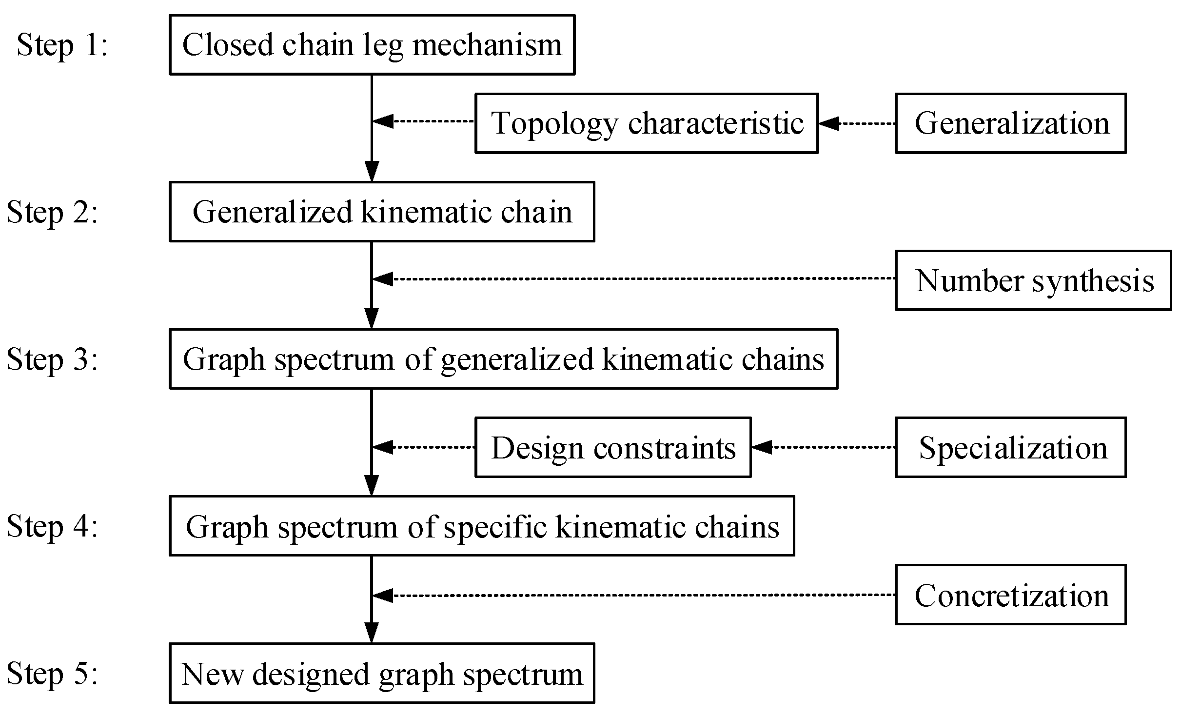
2.1. Selection of Closed-Chain Leg Structure

Figure 1 shows the flow chart used in the creative design of mechanical devices [33]. Based on this method, the closed kinematic chain (4,4)-type Chebyshev mechanism, the (6,7)-type Klanm mechanism [20], the (8,10)-type eight-link leg mechanism, and the (10,13)-type ten-link leg mechanism are proposed. The corresponding number of loops, the kinematic chains, and the number of non-isomorphic kinematic chains are also obtained. It can be concluded that the existing closed-chain leg mechanisms have several common structural characteristics. Their design constraints can be summarized as follows: (1) they have a single degree of freedom; (2) all kinematic pairs are flat low pairs; (3) they at least include crank rods, frame rods, thigh rods, and calf rods; (4) they have a crank rotation drive; and (5) the end of the calf rod generates a closed curve without a cross trajectory. Among them, the low accessory joint of the closed-chain leg mechanism can serve as a rotation joint or a sliding joint, and the sliding joint can be equivalent to a rotation joint with an infinite radius of curvature and is derived from a rotation joint.

For the (6,7), (8,10), and (10,13) kinematic chain types, the currently available closed-chain single-leg mechanisms are shown in

Table 1. Specific kinematic chain and closed-chain single-leg mechanisms.

(n,f)	(6,7)	(8,10)	(10,13)
Generalized kinematic chain
Specific kinematic chain
Schematic diagram of the new closed -chain leg mechanism

.

Type (4,4) is the simplest form of closed-chain single-leg mechanism. Besides the specifically allocated rods, there are no other rods for transmission connection, so the flexibility, diversity, and continuity of the mechanism are weak. At the same time, under the premise of having the same overall size, material, external load, and movement speed as the single-leg, the (4,4)-type single-loop structure is larger in size than the other three rods, and its mechanical properties are reduced. This leads to problems such as the slender rods’ compression instability, leg bending failures, an increase in crank motor torque, and so on. Meanwhile, the (6,7)-type, (8,10)-type, and (10,13)-type can achieve more sophisticated closed-chain leg mechanisms through creative design. From the perspective of engineering implementation, the number of closed-chain leg mechanism members and the complexity increase and the leg structure design will be more complicated; this also increases the weight of the mechanical body and the mechanical friction of the joints.

In summary, taking (6,7) as the basic form of the closed-chain single-leg mechanism, the diagram of the closed-chain single-leg mechanism is shown in

Table 2. The (6,7)-type of closed-chain leg mechanism.

Serial Number	1	2	3	4	5
Mechanism type	WATT-I	WATT-II	Stephenson-II	Stephenson-III	Stephenson-III
Specific kinematic chain
Schematic diagram of the new closed -chain leg mechanism

.

Based on the above-mentioned (6,7)-type new closed-chain leg mechanism design, the subsequent design of the closed-chain single-leg mechanism constructed via the Watt-I kinematic chain is shown in Figure 2.

2.2. Design Evaluation Index

Based on the design of the closed-chain single-leg mechanism, it is possible to build a quadruped walking platform. The design process of the multi-leg platform needs to be based on certain performance indicators.

First of all, the design of a closed-chain single leg should meet the following requirements: (1) the crank is driven by a single power to achieve revolving motion; (2) the foot end generates a closed, non-crossing trajectory that has a certain degree of symmetry; (3) the single leg should maintain straight support and a stable span as far as possible.

Secondly, the design of the whole closed-chain walking part should meet the following requirements: (1) the four-legged layout should be as compact as possible; (2) it should be composed of exactly the same single-leg mechanism; (3) there should be no mechanical interference during the movement of the four legs; (4) the drive should be located in the middle of the four legs; (5) the four-legged step sequence should ensure the stability of walking and reduce the impact vibration, center of mass fluctuations, and posture changes.

Finally, the design of the multi-leg carrier platform should meet the following requirements: (1) it should have a certain chassis height; (2) it should exhibit stable straight running and steering; (3) it should have good maneuverability, including rapidity and flexibility.

2.3. Degrees of Freedom Analysis of Closed-Chain Single-Leg Mechanism

As shown in Figure 3, the coordinate system of the closed-chain Watt-I type leg mechanism is established. The coordinates of each point are $A(x_A,y_A),B(x_B,y_B),C(x_C,y_C),$$(x_D,y_D),E(x_E,y_E),F(x_F,y_F),G(x_G,y_G)$. The uppercase letters and solid lines represent revolute joints and moving links, respectively. A triangle expresses a component.

According to the established coordinate system, the kinematic screw system of the closed-chain single-leg mechanism can be obtained as

$$\left\{\begin{array}{c}{\cancel{\mathit{S}}}_1=(001;000)\hfill \\ {\cancel{\mathit{S}}}_2=(001;y_B-x_{B}0)\hfill \\ {\cancel{\mathit{S}}}_3=(001;y_C-x_{C}0)\hfill \\ {\cancel{\mathit{S}}}_4=(001;y_D-x_{D}0)\hfill \\ {\cancel{\mathit{S}}}_5=(001;y_E-x_{E}0)\hfill \\ {\cancel{\mathit{S}}}_6=(001;y_F-x_{F}0)\hfill \\ {\cancel{\mathit{S}}}_7=(001;y_G-x_{G}0).\hfill \end{array}\right.$$

(1)

Among them, $(x_B,y_B),(x_C,y_C),(x_D,y_D),(x_E,y_E),(x_F,y_F),(x_G,y_G)$ are all different point coordinates. Since the first, second, and sixth elements in the Plücker coordinates of the seven screws are always zero, they have no impact on the configuration change. In this way, according to the calculation formula of the reciprocal product in the screw theory, namely $\cancel{\mathit{S}}·{\cancel{\mathit{S}}}^r$ = 0, we can obtain the constrained screw system of the seven screws as follows:

$$\left\{\begin{array}{c}{\cancel{\mathit{S}}}_1^r=(001;000)\hfill \\ {\cancel{\mathit{S}}}_2^r=(000;100)\hfill \\ {\cancel{\mathit{S}}}_3^r=(000;010).\hfill \end{array}\right.$$

(2)

Since there are three constraint screws, the mechanism has three public constraints and $\lambda$ = 3. The order of the mechanism is d = 6 − 3 = 3. In addition, $\nu$ and $\zeta$ are both 0. Thus, the degrees of freedom of the closed-chain single-leg mechanism are as follows:

$$M=6(n-g-1)+\sum _{i=1}^g{f}_i+\nu -\zeta =3(6-7-1)+7+0-0=1.$$

(3)

At the same time, ${\cancel{\mathit{S}}}_1^r$ is the constraint force along the Z axis, which constrains the movement along the Z axis. ${\cancel{\mathit{S}}}_2^r$ and ${\cancel{\mathit{S}}}_3^r$ are the couples around the X axis and the Y axis, respectively, restricting the rotation around the X axis and the Y axis, respectively.

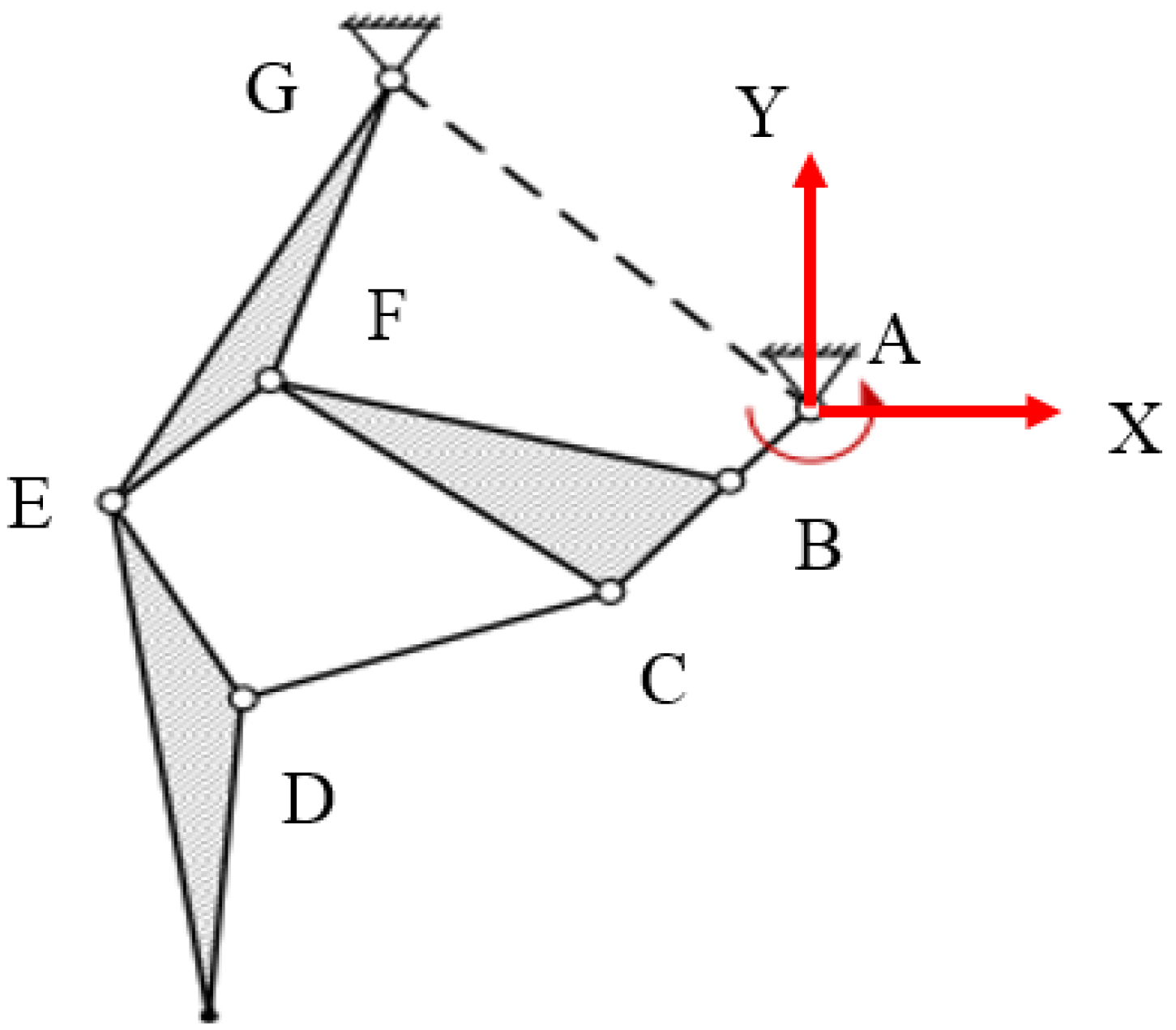
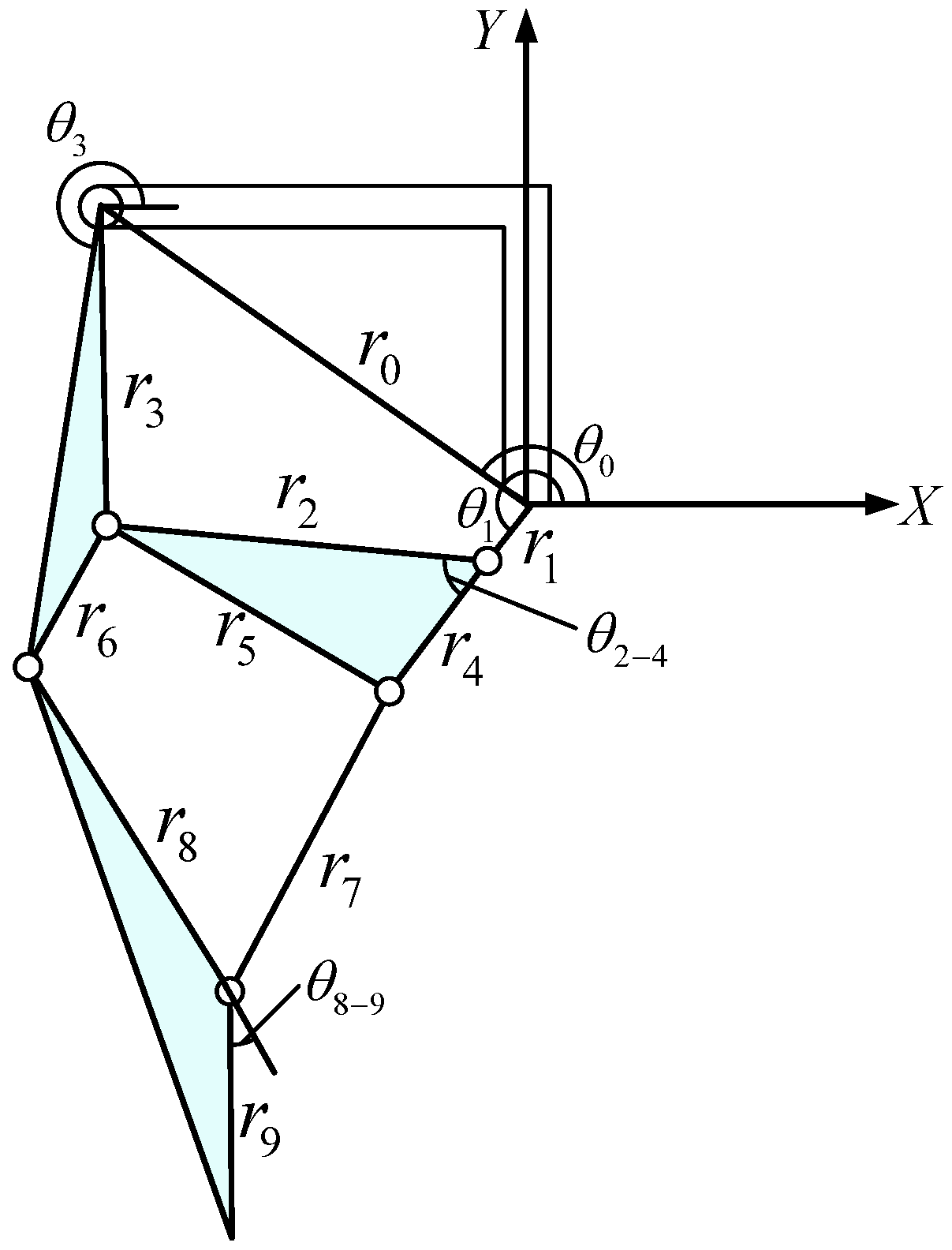
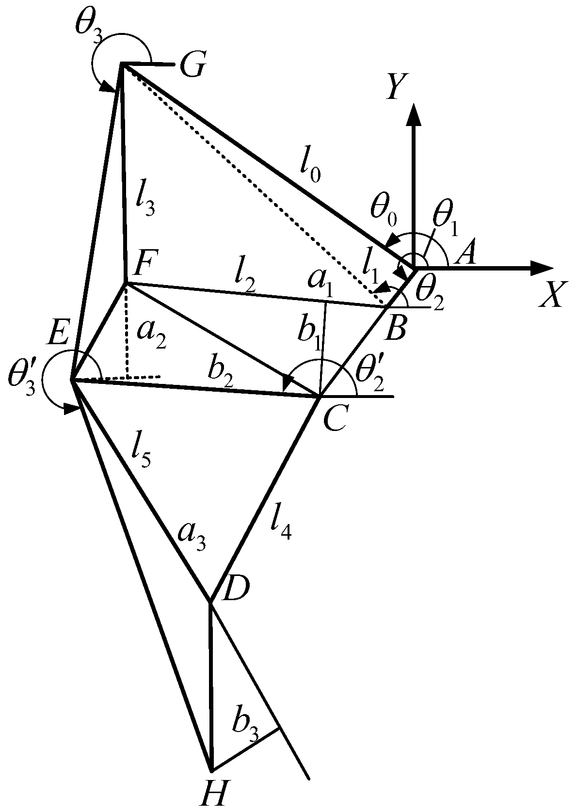
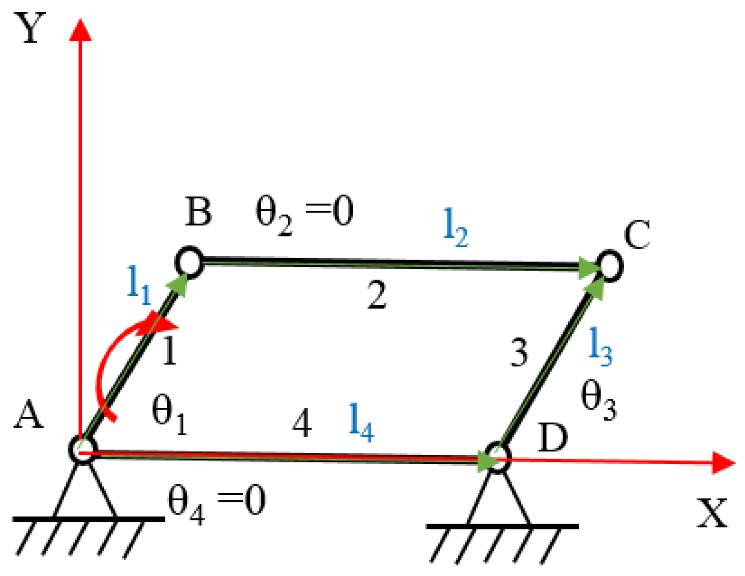
2.4. Kinematics Analysis of Closed-Chain Single-Leg Mechanism

For the closed-chain single-leg mechanism, we adopt the overall analysis method for the kinematic analysis. As shown in Figure 4, a rectangular coordinate system is established at the O point. The X axis is horizontal to the right, and the Y axis is vertically upward. The corresponding $\theta$ angles are the angles between the vector and the positive direction of the X axis. A blue triangle represents a component.

There are two closed loops in this mechanism, so two vector loop equations can be listed, which are expressed as follows:

$${\mathit{r}}_0+{\mathit{r}}_3-{\mathit{r}}_2-{\mathit{r}}_1={\mathbf{0}}_{2\times 1},$$

(4)

and

$${\mathit{r}}_5+{\mathit{r}}_6+{\mathit{r}}_7-{\mathit{r}}_8={\mathbf{0}}_{2\times 1}.$$

(5)

The vector of loop 1 (Equation (4)) is decomposed along the X and Y axes, and two trigonometric function equations are obtained:

$$r_{0}cos{\theta }_0+r_{3}cos{\theta }_3-r_{2}cos{\theta }_2-r_{1}cos{\theta }_1=0,$$

(6)

and

$$r_{0}sin{\theta }_0+r_{3}sin{\theta }_3-r_{2}sin{\theta }_2-r_{1}sin{\theta }_1=0,$$

(7)

where $r_0,{\theta }_0,r_3,r_2$, and $r_1$ are structural parameters, which are constants; ${\theta }_1$ is the rotation angle of the prime mover, which is a known parameter; and ${\theta }_2$ and ${\theta }_3$ are unknown.

After transforming Formulas (6) and (7) to solve ${\theta }_2$, we can obtain

$$r_{0}cos{\theta }_0-r_{2}cos{\theta }_2-r_{1}cos{\theta }_1=-r_{3}cos{\theta }_3,$$

(8)

and

$$r_{0}sin{\theta }_0-r_{2}sin{\theta }_2-r_{1}sin{\theta }_1=-r_{3}sin{\theta }_3.$$

(9)

Adding the squares of the two sides of the above formula, we can obtain

$$Acos{\theta }_2+Bsin{\theta }_2+C=0,$$

(10)

where

$$\left\{\begin{array}{c}A=2r_0{r}_{2}cos{\theta }_0-2r_1{r}_{2}cos{\theta }_1\hfill \\ B=2r_0{r}_{2}sin{\theta }_0-2r_1{r}_{2}sin{\theta }_1\hfill \\ C=-r_0^2-r_1^2-r_2^2+r_3^2+2r_0{r}_{1}cos({\theta }_0-{\theta }_1).\hfill \end{array}\right.$$

With order $t=tan{\displaystyle \frac{{\theta }_2}{2}}$, there are $sin{\theta }_2={\displaystyle \frac{2t}{1+t^2}},cos{\theta }_2={\displaystyle \frac{1-t^2}{1+t^2}}$. Substituting these into Equation (10), we can obtain

$$(C-A)t^2+2Bt+(A+C)=0,$$

(11)

where

$$\left\{\begin{array}{c}t={\displaystyle \frac{-B\pm \sqrt{B^2-C^2+A^2}}{C-A}}\hfill \\ {\theta }_2=2{tan}^{-1}\left(t\right),\hfill \end{array}\right.$$

and the above equation must satisfy $B^2-C^2+A^2\ge 0$.

In the same way, Formulas (6) and (7) are deformed and solved for ${\theta }_3$, and we can obtain

$$r_{0}cos{\theta }_0+r_{3}cos{\theta }_3-r_{1}cos{\theta }_1=r_{2}cos{\theta }_2,$$

(12)

and

$$r_{0}sin{\theta }_0+r_{3}sin{\theta }_3-r_{1}sin{\theta }_1=-r_{2}sin{\theta }_2.$$

(13)

Adding the squares of the two sides of the above formula, we can obtain

$$Acos{\theta }_3+Bsin{\theta }_3+C=0,$$

(14)

where

$$\left\{\begin{array}{c}A=2r_0{r}_{3}cos{\theta }_0-2r_1{r}_{3}cos{\theta }_1\hfill \\ B=2r_0{r}_{3}sin{\theta }_0-2r_1{r}_{3}sin{\theta }_1\hfill \\ C=r_0^2+r_1^2-r_2^2+r_3^2-2r_0{r}_{1}cos({\theta }_0-{\theta }_1).\hfill \end{array}\right.$$

With order $t=tan{\displaystyle \frac{{\theta }_3}{2}}$, there are $sin{\theta }_3={\displaystyle \frac{2t}{1+t^2}},cos{\theta }_3={\displaystyle \frac{1-t^2}{1+t^2}}$. Substituting these into Equation (14), we can obtain

$$(C-A)t^2+2Bt+(A+C)=0.$$

(15)

The solution is

$$\left\{\begin{array}{c}t={\displaystyle \frac{-B\pm \sqrt{B^2-C^2+A^2}}{C-A}}\hfill \\ {\theta }_3=2{tan}^{-1}\left(t\right),\hfill \end{array}\right.$$

and the above equation must satisfy $B^2-C^2+A^2\ge 0$.

Loop 2 (Formula (5)) is decomposed in the X and Y directions. Since ${\mathit{r}}_5={\mathit{r}}_2-{\mathit{r}}_4$, Formula (5) becomes

$${\mathit{r}}_2-{\mathit{r}}_4+{\mathit{r}}_6+{\mathit{r}}_8-{\mathit{r}}_7={\mathbf{0}}_{2\times 1}.$$

(16)

X direction decomposition results in

$$r_{2}cos{\theta }_2-r_{4}cos{\theta }_4+r_{6}cos{\theta }_6+r_{8}cos{\theta }_8-r_{7}cos{\theta }_7=0.$$

(17)

Y direction decomposition results in

$$r_{2}sin{\theta }_2-r_{4}sin{\theta }_4+r_{6}sin{\theta }_6+r_{8}sin{\theta }_8-r_{7}sin{\theta }_7=0,$$

(18)

where $r_2,r_4,{\theta }_2,{\theta }_4={\theta }_2+{\theta }_{2-4},r_6,{\theta }_6={\theta }_3+{\theta }_{3-6},r_8,r_7$ are all known quantities, and ${\theta }_7$ and ${\theta }_8$ are unknown quantities.

After transforming Equations (17) and (18) to solve ${\theta }_7$, we can obtain

$$r_{2}cos{\theta }_2-r_{4}cos{\theta }_4+r_{6}cos{\theta }_6-r_{7}cos{\theta }_7=-r_{8}cos{\theta }_8,$$

(19)

and

$$r_{2}sin{\theta }_2-r_{4}sin{\theta }_4+r_{6}sin{\theta }_6-r_{7}sin{\theta }_7=-r_{8}sin{\theta }_8.$$

(20)

After adding the squares of the two sides of the above formula, we simplify it to obtain

$$Acos{\theta }_7+Bsin{\theta }_7+C=0,$$

(21)

where

$$\left\{\begin{array}{c}A=-2r_2{r}_{7}cos{\theta }_2+2r_4{r}_{7}cos{\theta }_4-2r_6{r}_{7}cos{\theta }_6\hfill \\ B=-2r_2{r}_{7}sin{\theta }_2+2r_4{r}_{7}sin{\theta }_4-2r_6{r}_{7}sin{\theta }_6\hfill \\ C=r_2^2+r_4^2+r_6^2+r_7^2-r_8^2-2r_2{r}_{4}cos({\theta }_2-{\theta }_4)+2r_2{r}_{6}cos({\theta }_2-{\theta }_6)-2r_4{r}_{6}cos({\theta }_4-{\theta }_6).\hfill \end{array}\right.$$

With order $t=tan{\displaystyle \frac{{\theta }_7}{2}}$, there are $sin{\theta }_7={\displaystyle \frac{2t}{1+t^2}},cos{\theta }_7={\displaystyle \frac{1-t^2}{1+t^2}}$. Substituting these into Equation (21), we can obtain

$$(C-A)t^2+2Bt+(A+C)=0.$$

(22)

The solution is

$$\left\{\begin{array}{c}t={\displaystyle \frac{-B\pm \sqrt{B^2-C^2+A^2}}{C-A}}\hfill \\ {\theta }_7=2{tan}^{-1}\left(t\right),\hfill \end{array}\right.$$

and the above equation must satisfy $B^2-C^2+A^2\ge 0$.

In the same way, Formulas (17) and (18) are deformed and solved for ${\theta }_8$, and we can obtain

$$r_{2}cos{\theta }_2-r_{4}cos{\theta }_4+r_{6}cos{\theta }_6+r_{8}cos{\theta }_8=r_{7}cos{\theta }_7,$$

(23)

and

$$r_{2}sin{\theta }_2-r_{4}sin{\theta }_4+r_{6}sin{\theta }_6+r_{8}sin{\theta }_8=r_{7}sin{\theta }_7.$$

(24)

Adding the squares of the two sides of the above formula, we can obtain

$$Acos{\theta }_3+Bsin{\theta }_3+C=0,$$

(25)

where

$$\left\{\begin{array}{c}A=2r_2{r}_{8}cos{\theta }_2-2r_4{r}_{8}cos{\theta }_4+2r_6{r}_{8}cos{\theta }_6\hfill \\ B=2r_2{r}_{8}sin{\theta }_2-2r_4{r}_{8}sin{\theta }_4+2r_6{r}_{8}sin{\theta }_6\hfill \\ C=r_2^2+r_4^2+r_6^2+r_8^2-r_7^2-2r_2{r}_{4}cos({\theta }_2-{\theta }_4)+2r_2{r}_{6}cos({\theta }_2-{\theta }_6)-2r_4{r}_{6}cos({\theta }_4-{\theta }_6).\hfill \end{array}\right.$$

With order $t=tan{\displaystyle \frac{{\theta }_8}{2}}$, there are $sin{\theta }_8={\displaystyle \frac{2t}{1+t^2}},cos{\theta }_8={\displaystyle \frac{1-t^2}{1+t^2}}$. Substituting these into Equation (25), we can obtain

$$(C-A)t^2+2Bt+(A+C)=0.$$

(26)

The solution is

$$\left\{\begin{array}{c}t={\displaystyle \frac{-B\pm \sqrt{B^2-C^2+A^2}}{C-A}}\hfill \\ {\theta }_8=2{tan}^{-1}\left(t\right),\hfill \end{array}\right.$$

and the above equation must satisfy $B^2-C^2+A^2\ge 0$.

The leg-end position can be calculated according to the vector ${\mathit{r}}_1+{\mathit{r}}_4+{\mathit{r}}_7+{\mathit{r}}_9$, where the angle corresponding to the vector ${\mathit{r}}_1$ is ${\theta }_1$, the angle corresponding to the vector ${\mathit{r}}_4$ is ${\theta }_4={\theta }_2+{\theta }_{2-4}$, the angle corresponding to the vector ${\mathit{r}}_7$ is ${\theta }_7$, and the angle corresponding to the vector ${\mathit{r}}_9$ is ${\theta }_9={\theta }_8+{\theta }_{8-9}$.

The X direction coordinate of the leg end is

$$X=r_{1}cos{\theta }_1+r_{4}cos{\theta }_4+r_{7}cos{\theta }_7+r_{9}cos{\theta }_9.$$

(27)

The Y direction coordinate of the leg end is

$$Y=r_{1}sin{\theta }_1+r_{4}sin{\theta }_4+r_{7}sin{\theta }_7+r_{9}sin{\theta }_9.$$

(28)

Deriving both ends of Equations (6) and (7) according to time, the angular velocity $\omega$ can be obtained as

$$-{\omega }_3{r}_{3}sin{\theta }_3+{\omega }_2{r}_{2}sin{\theta }_2-{\omega }_1{r}_{1}sin{\theta }_1=0,$$

(29)

and

$${\omega }_3{r}_{3}cos{\theta }_3{\omega }_2{r}_{2}cos{\theta }_2+{\omega }_1{r}_{1}cos{\theta }_1=0.$$

(30)

Combined with the above formulas, we can obtain

$${\omega }_2={\displaystyle \frac{{\omega }_1{r}_{1}sin({\theta }_3-{\theta }_1)}{r_{2}sin({\theta }_2-{\theta }_3)}},$$

(31)

and

$${\omega }_3={\displaystyle \frac{{\omega }_1{r}_{1}sin({\theta }_2-{\theta }_1)}{r_{2}sin({\theta }_2-{\theta }_3)}}.$$

(32)

We solve both sides of Equations (17) and (18) to obtain

$${\omega }_7={\displaystyle \frac{r_2{\omega }_{2}sin({\theta }_2-{\theta }_8)+r_4{\omega }_{4}sin({\theta }_8-{\theta }_4)}{r_{2}sin({\theta }_7-{\theta }_8)}}+{\displaystyle \frac{r_6{\omega }_{6}sin({\theta }_6-{\theta }_8)}{r_{8}sin({\theta }_7-{\theta }_8)}},$$

(33)

and

$${\omega }_8={\displaystyle \frac{r_2{\omega }_{2}sin({\theta }_2-{\theta }_7)+r_4{\omega }_{4}sin({\theta }_7-{\theta }_4)}{r_{8}sin({\theta }_7-{\theta }_8)}}+{\displaystyle \frac{r_6{\omega }_{6}sin({\theta }_6-{\theta }_7)}{r_{8}sin({\theta }_7-{\theta }_8)}},$$

(34)

where ${\omega }_2={\omega }_4,{\omega }_3={\omega }_6$, ${\omega }_1$ is the angular velocity of the drive motor.

The second-order derivative with respect to time in Equations (6), (7), (17) and (18) can be used to calculate the accelerations of four unknown angles, which are recorded as ${\alpha }_2,{\alpha }_3,{\alpha }_7,$ and ${\alpha }_8$, respectively. The unknown angular acceleration can be calculated as follows:

$$\left\{\begin{array}{c}{\alpha }_2={\displaystyle \frac{Ecos{\theta }_3+Fsin{\theta }_3}{r_{2}sin({\theta }_2-{\theta }_3)}}\hfill \\ {\alpha }_3={\displaystyle \frac{Ecos{\theta }_2+Fsin{\theta }_2}{r_{3}sin({\theta }_2-{\theta }_3)}}\hfill \\ {\alpha }_7={\displaystyle \frac{Ecos{\theta }_8+Fsin{\theta }_8}{r_{7}sin({\theta }_7-{\theta }_8)}}\hfill \\ {\alpha }_8={\displaystyle \frac{Ecos{\theta }_7+Fsin{\theta }_7}{r_{8}sin({\theta }_7-{\theta }_8)}},\hfill \end{array}\right.$$

(35)

where

$$\left\{\begin{array}{c}E=r_0{\omega }_0^{2}cos{\theta }_0+r_3{\omega }_3^{2}cos{\theta }_3-r_2{\omega }_2^{2}cos{\theta }_2-r_1{\omega }_1^{2}cos{\theta }_1\hfill \\ F=r_0{\omega }_0^{2}sin{\theta }_0+r_3{\omega }_3^{2}sin{\theta }_3-r_2{\omega }_2^{2}sin{\theta }_2-r_1{\omega }_1^{2}sin{\theta }_1\hfill \\ G=r_2{\omega }_2^{2}cos{\theta }_2-r_4{\omega }_4^{2}cos{\theta }_4+r_6{\omega }_6^{2}cos{\theta }_6+r_8{\omega }_8^{2}cos{\theta }_8-r_7{\omega }_7^{2}cos{\theta }_7+\hfill \\ r_2{\alpha }_{2}sin{\theta }_2-r_4{\alpha }_{4}sin{\theta }_4+r_6{\alpha }_{6}sin{\theta }_6\hfill \\ H=r_2{\omega }_2^{2}sin{\theta }_2-r_4{\omega }_4^{2}sin{\theta }_4+r_6{\omega }_6^{2}sin{\theta }_6+r_8{\omega }_8^{2}sin{\theta }_8-r_7{\omega }_7^{2}sin{\theta }_7+\hfill \\ r_2{\alpha }_{2}sin{\theta }_2-r_4{\alpha }_{4}sin{\theta }_4+r_6{\alpha }_{6}sin{\theta }_6.\hfill \end{array}\right.$$

(36)

Thus far, all unknown angular displacements $({\theta }_2,{\theta }_3,{\theta }_4,{\theta }_6,{\theta }_7,{\theta }_8,{\theta }_9)$, angular velocities $({\omega }_2,{\omega }_3,{\omega }_4,{\omega }_6,{\omega }_7,{\omega }_8,{\omega }_9)$, and angular accelerations $({\alpha }_2,{\alpha }_3,{\alpha }_4,{\alpha }_6,{\alpha }_7,{\alpha }_8,{\alpha }_9)$ involved in the two loops have been calculated.

Through analysis and programming with the MATLAB (2017b) software, the leg-end motion trajectory of the single-leg closed chain mechanism is obtained.

2.5. Singularity Analysis of Closed-Chain Single-Leg Mechanism

The Watt-I type closed-chain single-leg mechanism has a single degree of freedom and can be divided into a planar four-bar mechanism and a class II linkage group. In reference [34], it is considered that the singularity analysis of a planar multi-ring mechanism can be divided according to the basic rod group. When a basic rod group reaches the singular position type, the complex mechanism is of the singular position type. Based on this principle, the singularity of the planar four-bar mechanism is analyzed.

For the four-bar linkage, the axes of the four rotating pairs are parallel to each other. They can be expressed as four line vectors with a zero pitch of ${\cancel{\mathit{S}}}_1,{\cancel{\mathit{S}}}_2,{\cancel{\mathit{S}}}_3,{\cancel{\mathit{S}}}_4$. We place the origins of the coordinates at point A, and the four kinematic pairs form a screw system ${\left[\mathit{J}\right]}^T$ as follows:

$${\left[\mathit{J}\right]}^T=\left[\begin{array}{c}{\cancel{\mathit{S}}}_1\\ {\cancel{\mathit{S}}}_2\\ {\cancel{\mathit{S}}}_3\\ {\cancel{\mathit{S}}}_4\end{array}\right]=\left[\begin{array}{cccccc}0& 0& 1& 0& 0& 0\\ 0& 0& 1& y_B& x_B& 0\\ 0& 0& 1& y_C& x_C& 0\\ 0& 0& 1& y_D& x_D& 0\end{array}\right],$$

(37)

where $y_i,x_i,(i=B,C,D)$ can be obtained from the positive solutions.

Obviously, in this 4 × 6 matrix, only a 4 × 3 sub-matrix ${\left[{\mathit{J}}^S\right]}^T$ is effective.

$${\left[{\mathit{J}}^S\right]}^T=\left[\begin{array}{ccc}1& 0& 0\\ 1& y_B& x_B\\ 1& y_C& x_C\\ 1& y_D& x_D\end{array}\right].$$

(38)

The rank of ${\left[{\mathit{J}}^S\right]}^T$ is 3 at most, so the four spirals ${\cancel{\mathit{S}}}_1,{\cancel{\mathit{S}}}_2,{\cancel{\mathit{S}}}_3,{\cancel{\mathit{S}}}_4$ are linearly related and belong to a three-series spiral, which can be expressed as

$$\sum _{j=1}^4{\omega }_j{\cancel{\mathit{S}}}_j=0.$$

(39)

For the spatial three-phase screw, there are three reciprocals that are inverse to it, i.e., three common constraints are imposed on the plane mechanism. They are the force along the Z direction ${\cancel{\mathit{S}}}_1^r$ and the force couple vectors along the X and Y directions ${\cancel{\mathit{S}}}_2^r,{\cancel{\mathit{S}}}_3^r$:

$$\left\{\begin{array}{c}{\cancel{\mathit{S}}}_1^r=(001;000)\hfill \\ {\cancel{\mathit{S}}}_2^r=(000;100)\hfill \\ {\cancel{\mathit{S}}}_3^r=(000;010).\hfill \end{array}\right.$$

(40)

For a four-bar mechanism, when ${\cancel{\mathit{S}}}_1^r,{\cancel{\mathit{S}}}_2^r,{\cancel{\mathit{S}}}_3^r$ are coplanar, the mechanism is at the limit displacement singularity; when ${\cancel{\mathit{S}}}_2^r,{\cancel{\mathit{S}}}_3^r,{\cancel{\mathit{S}}}_4^r$ are coplanar, the mechanism is at the dead-point singularity; when ${\cancel{\mathit{S}}}_3^r,{\cancel{\mathit{S}}}_4^r$ are coplanar, the mechanism is at the instantaneous degree of freedom change singularity; when ${\cancel{\mathit{S}}}_1^r,{\cancel{\mathit{S}}}_2^r,{\cancel{\mathit{S}}}_3^r,{\cancel{\mathit{S}}}_4^r$ are coaxial, the mechanism is at the continuous geometric singularity.

(1) The limit displacement singularity

When the limit displacement is singular, ${\cancel{\mathit{S}}}_1^r,{\cancel{\mathit{S}}}_2^r,{\cancel{\mathit{S}}}_3^r$ are coplanar, i.e.,

$$det\left(\left[\begin{array}{ccc}1& 0& 0\\ 1& y_B& x_B\\ 1& y_C& x_C\end{array}\right]\right)=0.$$

(41)

If and only if $y_B·x_C-y_C·x_B=0$, points A, B, and C are collinear. We solve the input variable $\theta$ at this time, and the input variable $\theta$ is obtained as

$$\theta =arccos\left({\displaystyle \frac{{(a+b)}^2+d^2-c^2}{2d(a+b)}}\right),$$

(42)

or

$$\theta =arccos\left({\displaystyle \frac{{(a-b)}^2+d^2-c^2}{2d(a-b)}}\right),$$

(43)

where $a,b,c,d$ represent the rod length AB, BF, FG, GA, respectively.

(2) The limit displacement singularity

When the limit displacement is singular, ${\cancel{\mathit{S}}}_2^r,{\cancel{\mathit{S}}}_3^r,{\cancel{\mathit{S}}}_4^r$ are coplanar, i.e.,

$$det\left(\left[\begin{array}{ccc}1& y_B& x_B\\ 1& y_C& x_C\\ 1& y_D& x_D\end{array}\right]\right)=0.$$

(44)

If and only if $(y_C-y_B)(x_D-x_B)-(y_D-y_B)(x_c-x_B)=0$, points B, C, and D are collinear. However, since $a+d<b+c$ in this study, there will be no dead point singularity.

(3) Singularity of instantaneous change in degree of freedom

When ${\cancel{\mathit{S}}}_2^r,{\cancel{\mathit{S}}}_3^r,{\cancel{\mathit{S}}}_4^r$ are coplanar, the mechanism has an instantaneously changing degree of freedom. The mechanism has two degrees of freedom instantaneously, corresponding to each $3\times 3$ sub-formula of the ${\left[{\mathit{J}}^S\right]}^T$ matrix, and the determinants are all 0 at the same time.

Since the determinant of its sub-formulas $\left[\begin{array}{ccc}1& y_B& x_B\\ 1& y_C& x_C\\ 1& y_D& x_D\end{array}\right]$ must not be zero, there is no singularity in the instantaneous change in the degrees of freedom.

(4) Continuous geometric singularity

When ${\cancel{\mathit{S}}}_1^r,{\cancel{\mathit{S}}}_3^r$ or ${\cancel{\mathit{S}}}_2^r,{\cancel{\mathit{S}}}_4^r$ are coaxial, the mechanism is in continuous geometric singularity. In other words, $\left[\begin{array}{ccc}1& y_B& x_B\\ 1& y_D& x_D\end{array}\right]$ or $\left[\begin{array}{ccc}1& y_A& x_A\\ 1& y_C& x_C\end{array}\right]$ have a linear correlation, which means that $a=c$ or $b=d$ is strictly required, so there is no self-continuous geometric singularity.

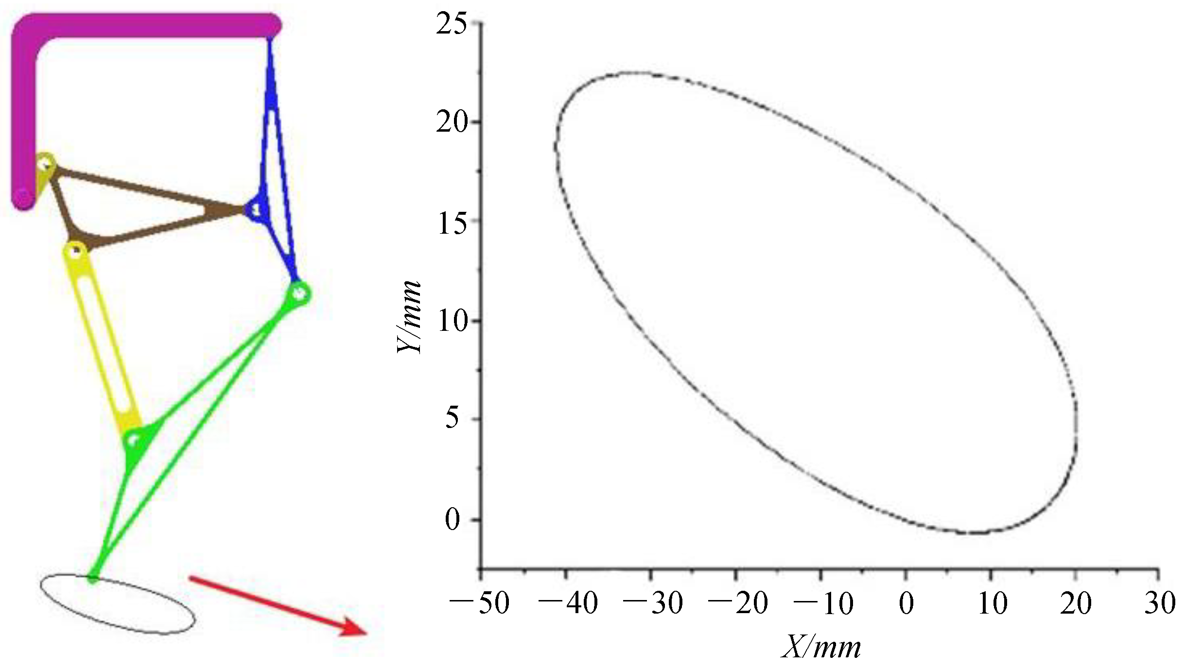
3. Mechanism Size Optimization Based on Trajectory Reproduction

3.1. Basic Research Methods

Trajectory reproduction is the method of reversing the size of the mechanism through the set ideal trajectory curve [35]. For general machines with leg structures, it is often an important aspect of dimension synthesis to obtain a mechanism with a predetermined trajectory. The results show that the foot-end trajectory with a small leg-lifting height and large proportion of support is suitable for fast-moving robots, and the foot-end track with a high leg-lifting height is suitable for obstacle-crossing robots.

For the dimensional optimization of trajectory reproduction, the trial-and-error method and drawing method can be used. However, for a complex mechanism with multiple structural parameters, the trial-and-error method needs a large amount of time and cannot guarantee the optimality of the results. The drawing method is not suitable for complex mechanisms and is almost infeasible. In this study, the inverse trajectory problem is transformed into an equivalent nonlinear optimization model with constraints, and the related algorithm optimization method is used to solve the problem to a certain extent.

3.2. Trajectory Reconstruction Based on Traditional Algorithms

3.2.1. Establish an Equivalent Nonlinear Optimization Model with Constraints

For a Watt-I-type structure, if $x_a=0$ and $y_a=0$ are set, the driving angle ${\phi }_1$ and 13 structural parameters $(l_1,l_2,l_3,l_4,l_5,x_g,y_g,a_1,a_2,a_3,b_1,b_2,b_3)$ are required. They can determine the mechanism, as shown in Figure 5.

When the driving angle ${\phi }_1$ of the active part is determined, the foot-end trajectory $x_h,y_h$ is a function of these 13 structural parameters:

$$\left\{\begin{array}{c}{x}_h=f_1\left(l_1,l_2,l_3,l_4,l_5,x_g,y_g,a_1,a_2,a_3,b_1,b_2,b_3\right)\hfill \\ y_h=f_2\left(l_1,l_2,l_3,l_4,l_5,x_g,y_g,a_1,a_2,a_3,b_1,b_2,b_3\right).\hfill \end{array}\right.$$

We artificially design a preset trajectory and select some points $(x_h^{\prime },y_h^{\prime })$ from the trajectory for approximation. Then, we construct the objective function:

$$min\left[f\left(x\right)\right]=min\left[\sum _{i=1}^6{(x_h-x_h^{\prime })}^2+{(y_h-y_h^{\prime })}^2\right]=0.$$

(45)

The construction of the constraint conditions includes the existence condition of the crank of the four-bar mechanism and the existence condition of the rod length:

$$S.t.\left\{\begin{array}{c}{l}_1<l_2\hfill \\ l_1<l_3\hfill \\ l_1<l_6\hfill \\ l_1+l_2<l_1+l_3\hfill \\ l_1+l_3<l_2+l_6\hfill \\ l_1+l_6<l_2+l_6\hfill \\ \left(l_1,l_2,l_3,l_4,l_5,x_g,y_g,a_1,a_2,a_3,b_1,b_2,b_3\right)>0.\hfill \end{array}\right.$$

(46)

3.2.2. Establish Result Evaluation Model

The typical algorithms for constrained nonlinear optimization models include quadratic sequential programming (SQP) [36], the interior-point method, and the active-set method. The traditional algorithm needs to be given an initial value when solving. In order to verify the feasibility of the three algorithms, a set of ideal parameters is set, as shown in

Table 3. Ideal structural parameters of the proposed foot mobile robot.

Parameters	Numerical Value (mm)	Parameters	Numerical Value (mm)
$l_1$	15.9	$a_2$	105
$x_g$	−96.9	$b_2$	18.5
$y_g$	70.4	$l_4$	78.2
$l_2$	87.4	$l_5$	87.9
$l_3$	73.1	$a_3$	126.2
$a_1$	19.3	$b_3$	29.2
$b_1$	31.8

, and the trajectory leg-end trace is shown in Figure 6. Moreover, six points are selected for approximation, which are shown in

Table 4. The coordinates of six approach points selected on the trajectory.

${\mathit{\phi }}_1$ (deg)	0	60	120	180	240	300
${\mathit{x}}_h^{\prime }$ (mm)	−22.368	−9.6286	−30.5297	−63.0965	−69.6808	−50.6535
${\mathit{y}}_h^{\prime }$ (mm)	−162.530	−151.182	−149.276	−157.858	−168.004	−170.216

.

The initial value is obtained by accumulating some errors according to the ideal value, which is expressed as

$$q_{i^{\prime }}=q_i+\Delta ,$$

(47)

where $q_i$ represents the ideal values of the thirteen structural parameters, and $q_{i^{\prime }}$ represents the corresponding calculated value.

We set the error evaluation function:

$$g\left(x\right)=\sum _{i=1}^{13}{(q-q_i)}^2,(i=1,2,\cdots ,13),$$

(48)

where $g\left(x\right)$ approaches 0, indicating that the effect is better.

3.2.3. Experimental Verification

We select the initial errors of 1, 3, 5, 7, 9, and 11 and use three algorithms adopted to solve constrained nonlinear optimization problems. The quadratic sequential programming method (SQP), interior-point method, and active-set method are used for error calculation. The results are shown in

Table 5. Error calculation results of different optimization algorithms.

Method/Initial   Error $\mathbf{\Delta }$	1 mm	3 mm	5 mm	7 mm	9 mm	11 mm
SQP	4	402	1502	8206	17,483	28,606
Interior point	1	1	33	9791	10,810	9868
Active set	1	18	87	13,634	32,300	27,356

. The data show that the three methods of solving the nonlinear optimization problem can alleviate the problem of trajectory inversion within a certain initial value error range. However, for the mechanism involved in this study, when the initial value error is greater than 5 mm, the solution effect will drop sharply. In fact, 5 mm is “insignificant” relative to the overall size of the mechanism. In other words, the above three algorithms are “over-dependent” on the initial value, which often has no use value in actual engineering. Similarly, it is also proven that the phenomenon of the oversensitivity to the initial value increases the complexity of the mechanism.

Therefore, the traditional algorithm used to solve the constrained nonlinear optimization problem is not suitable for the trajectory inversion problems of complex mechanisms.

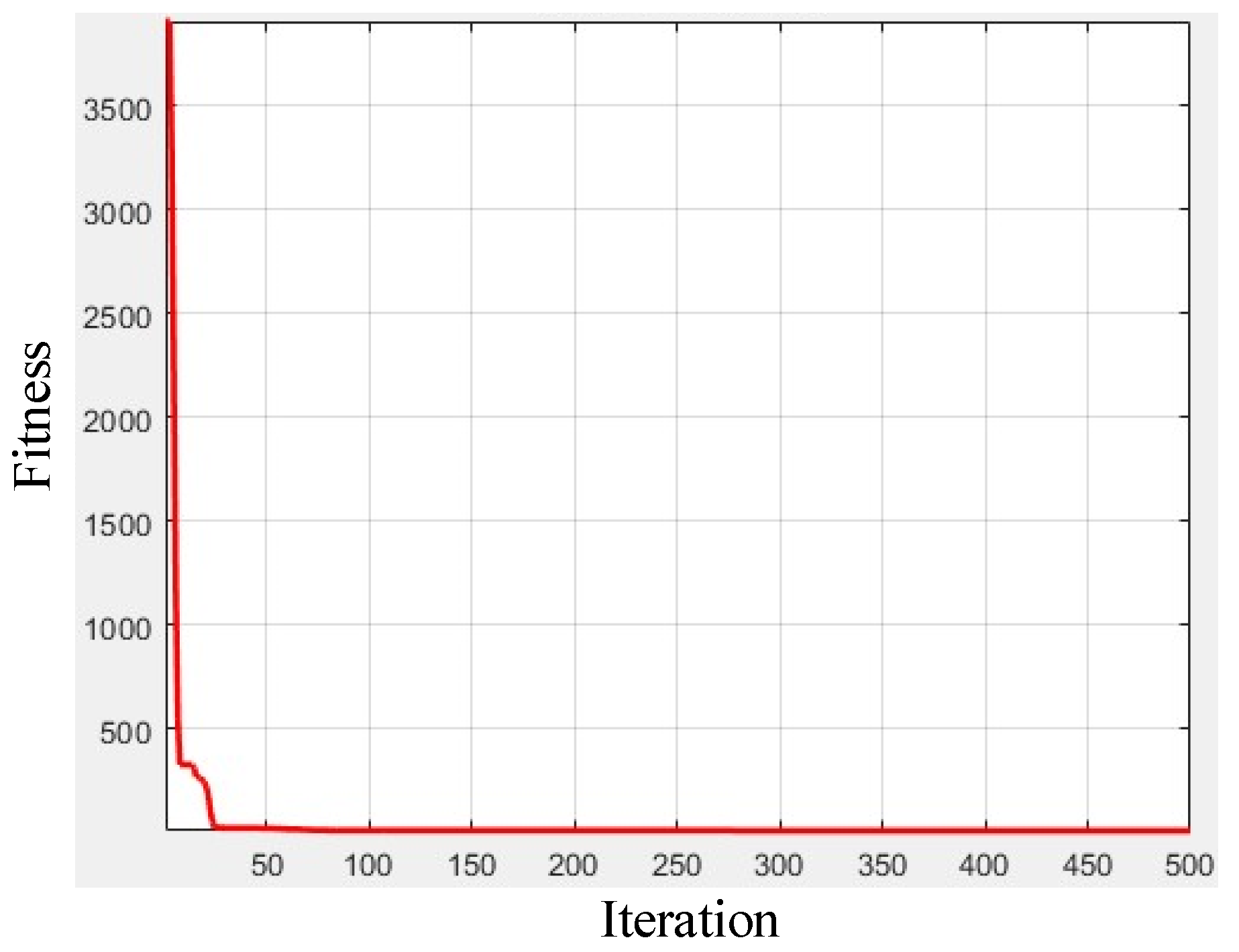
3.3. Trajectory Reconstruction Problem Based on Heuristic Algorithm

Common heuristic algorithms include the genetic algorithm, particle swarm algorithm, simulated annealing algorithm, etc. These algorithms are derived from different physical, chemical, and biological phenomena in the natural world [37]. This study uses the particle swarm algorithm to solve the trajectory reversal problem.

3.3.1. The Idea of the Particle Swarm Algorithm

The particle swarm algorithm was proposed in 1995, and its idea originated from the biological phenomenon of birds looking for food. The particle swarm algorithm searches for the optimal solution in the solution space through group iteration. Due to its simplicity, fast convergence speed, and small number of parameters, it has been widely used in various fields. The optimal solution can be regarded as food, and a flock of birds searches for the food in the solution space at a certain speed. The birds do not know where the food is, but they can perceive the distance to the food as a whole (objective function). The strategy adopted to find the food is as follows: all birds approach the bird closest to the food and search for the nearest one, with one loop iteration. The solution of each optimization problem is regarded as a bird, i.e., a “particle”, and all particles search for the optimal solution in the D-dimensional solution space. D is determined by the dimensions of the parameters. Each particle is defined by a fitness function to determine the quality of the current position, and each particle can remember the best area searched. Each particle adjusts the direction and speed of flight by receiving group information to approach the optimal solution.

3.3.2. Experimental Verification

The selected model parameters are shown in

Table 6. PSO algorithm parameters.

Particle Swarm Scale	The Maximum Number of Iterations	Inertia Weight	Learning Factor ${\mathit{c}}_1$	Learning Factor ${\mathit{c}}_2$	Particle Velocity
500	500	0.7298	1.4961	1.4961	[−1, 1]

.

The calculated and theoretical values of the 13 parameters obtained through iteration are shown in

Table 7. Calculated and theoretical values of parameters.

${\mathit{q}}_{\mathit{i}}$	Theoretical Value (mm)	Calculated Value (mm)
$l_1$	15.9	15.9
$x_g$	−96.9	−93.9
$y_g$	70.4	79.0
$l_2$	87.4	85.2
$l_3$	73.1	78.1
$a_1$	19.3	7.43
$b_1$	31.8	42.3
$a_2$	105	111
$b_2$	18.5	18.8
$l_4$	78.2	75.8
$l_5$	87.9	102
$a_3$	126.2	137
$b_3$	29.2	33.5

.

The curve of the iterative algebra and individual fitness is shown in Figure 7. The abscissa represents the evolutionary algebra, and the ordinate represents the fitness.

The trajectory obtained by bringing the calculated value into the positive kinematics solution is shown in Figure 8. It is basically consistent with the target trajectory.

In summary, it can be seen that the heuristic algorithm used to solve the trajectory reversal problem is far better than the traditional algorithm. Although there are small differences in some parameters, the overall trajectories are almost consistent. The greater the number of fitting points selected when establishing the objective function, the more accurate the solution, and the less likely it is to fall into local optima.

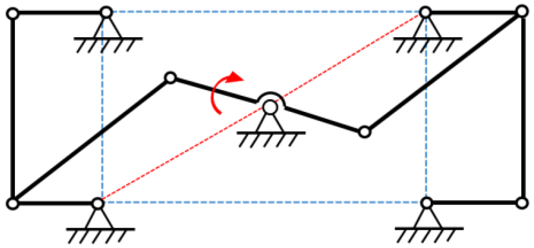
4. Design and Analysis of Steering Mechanism

4.1. Design and Selection of Steering Mechanism

After determining the closed-chain single-leg mechanism of the parallel foot robot and its arrangement and position on the platform, it is necessary to design the steering mechanism for the legs in order to realize the synchronous steering function of the four closed-chain leg structures of the legged robot. The design requirement is that the leg has a rotation range of at least 90°. Based on this, a motor-synchronous structure or a motor-rod group structure can be used. Among them, synchronous belts mostly use rubber, which is an elastic member and can easily be thermally aged, deformed, elongated, or broken. Moreover, it is not suitable for long-distance transmission. When the car body size is large, the transmission effect is worsened. In contrast, the reliability and accuracy of the motor-rod group is higher, and the following two structures are proposed.

Structure 1: The driving rod has an angle and forms a general four-bar mechanism with other rods, as shown in Figure 9. The red arrow represents the rotation direction of the driving link, and the dashed line indicates that the revolute joints on it are collinear.

Structure 2: The driving rod is arranged horizontally, and it forms a parallelogram mechanism with other rods, as shown in Figure 10.

The difference between the two structures is the length of the driving link. Considering the parallelogram mechanism, as shown in Figure 11a, its movement characteristics are as follows: the driving crank and the driven crank have the same rotation speed and direction, and the connecting link always moves horizontally. In order to control the rotation angle of the closed-chain leg structure, the parallelogram mechanism of Structure 2 is selected as the steering structure. The initial position is shown in Figure 11b, and the limit position is shown in Figure 11c.

The placement positions of the four closed-chain single-leg mechanisms of the robot on the platform (as shown in Figure 12), i.e., A, B, C, and D, have been determined. In order to realize the synchronous steering of the foot robot, the diagonal midpoint O is selected for use as the center of the driving link. The distance of the AO section is known, and the length of link AE is unknown. Considering that the length of the link AE cannot exceed half of the platform width AB, and the two closed-chain single-leg mechanisms on the same side cannot interfere with each other when turning, the length of link AE is determined to be 60 mm in the experiment.

Finally, the overall structure of the walking foot robot is designed, which is shown in Figure 13.

4.2. Analysis of Steering Mechanism

4.2.1. Calculation of Degrees of Freedom

The movement diagram of the steering mechanism is shown in Figure 14. According to the degrees of freedom calculation method for the planar mechanism, the number of degrees of freedom can be obtained. This value is calculated as follows:

$$F=3n-2P_1-P_h=3\times 9-2\times 13-0=1.$$

(49)

Therefore, the number of degrees of freedom of the steering mechanism is 1.

4.2.2. Kinematics Analysis

The core structure of the steering mechanism to achieve steering adopts the parallelogram structure, as shown in Figure 15.

Therefore, the parallelogram structure is taken for further analysis. As shown in Figure 16, we take point A as the origin to establish a rectangular coordinate system. We suppose that the length of member 1 is $l_1$, its azimuth angle is ${\theta }_1$, and $l_1$ is the rod vector of member 1, namely $l_1$ = AB. The rest of the components in the mechanism can all be expressed as corresponding rod vectors, so that a closed vector polygon composed of each rod vector is formed, namely ABCDA. In this closed vector polygon, the sum of its vectors must be equal to zero, i.e.,

$${\mathit{l}}_1+{\mathit{l}}_2-{\mathit{l}}_3-{\mathit{l}}_4={\mathbf{0}}_{2\times 1}.$$

(50)

(1) Location analysis

The closed vector Equation (50) of the mechanism is written as a projection on two coordinate axes and then rewritten in a form with only an unknown quantity on the left side of the equation. Thus, we have

$$\left\{\begin{array}{c}{l}_2-l_{3}cos{\theta }_3=l_4-l_{1}cos{\theta }_1\hfill \\ -l_{3}sin{\theta }_3=-l_{1}sin{\theta }_1.\hfill \end{array}\right.$$

(51)

It can be found that ${\theta }_1={\theta }_3$.

(2) Velocity analysis

Taking the first derivative of Equation (51) for time, we can obtain the following results:

$$\left\{\begin{array}{c}{l}_3{\omega }_3{sin}_3=l_1{\omega }_1{sin}_1\hfill \\ -l_3{\omega }_3{cos}_3=-l_1{\omega }_1{cos}_1.\hfill \end{array}\right.$$

(52)

It can be found that ${\omega }_1={\omega }_3$.

(3) Acceleration analysis

Taking the derivative of Equation (52) for time, we can obtain the acceleration formulas

$$\left\{\begin{array}{c}{l}_3{\alpha }_{3}cos{\theta }_3=l_1{\alpha }_{1}cos{\theta }_1\hfill \\ l_3{\alpha }_{3}sin{\theta }_3=l_1{\alpha }_{1}sin{\theta }_1.\hfill \end{array}\right.$$

(53)

It can be found that ${\alpha }_1={\alpha }_3$. The analysis shows that the velocity and acceleration relationship between input link AB and output link CD can be easily controlled to control the motion parameters of the steering structure.

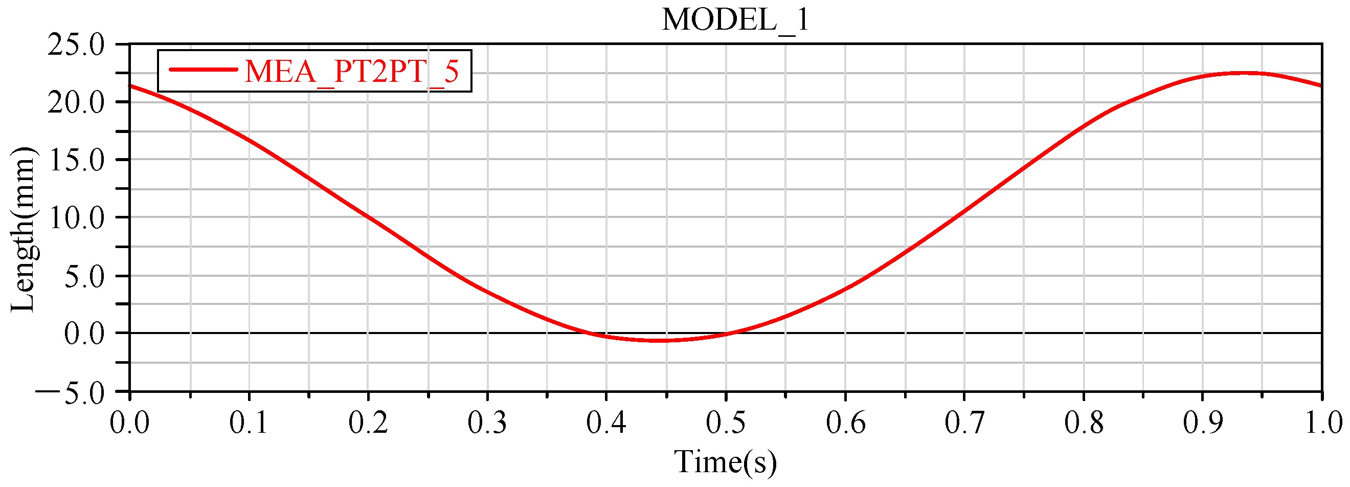
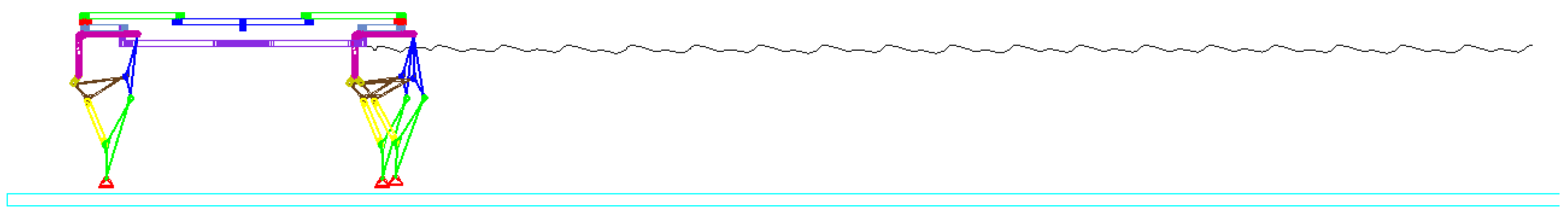
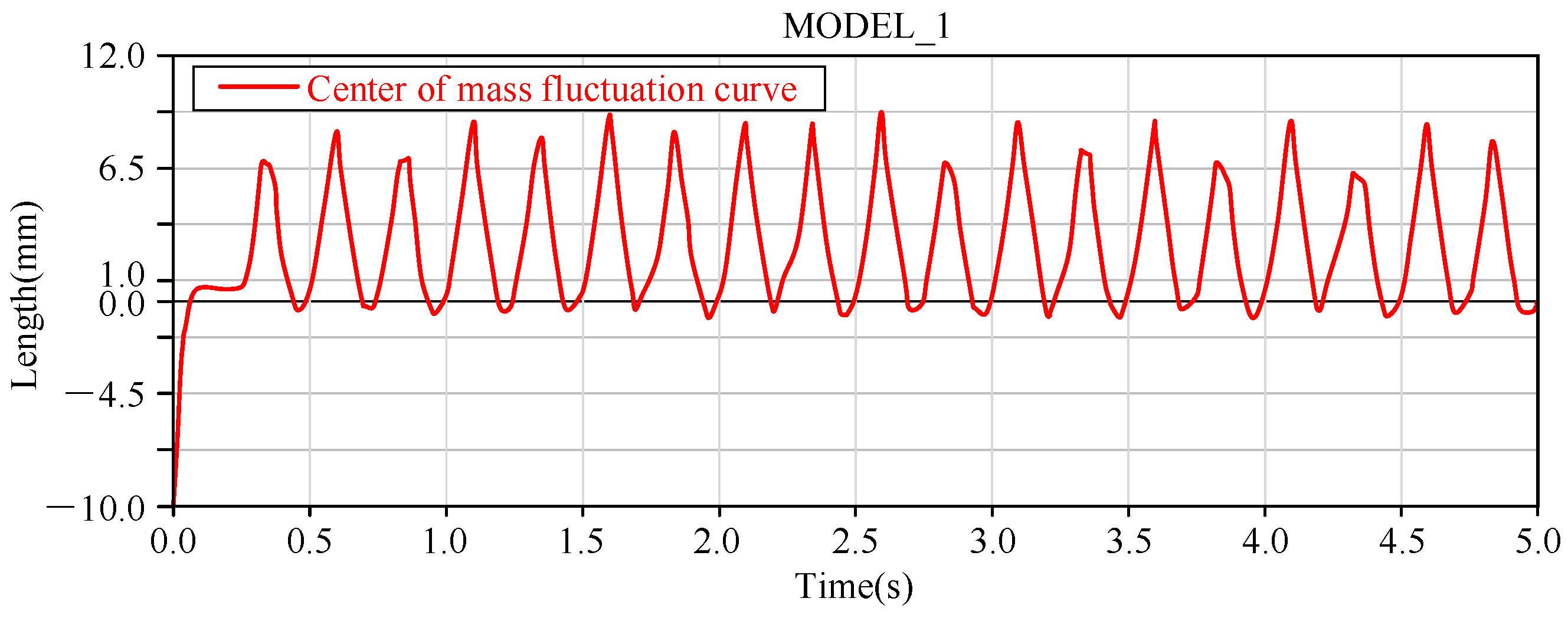
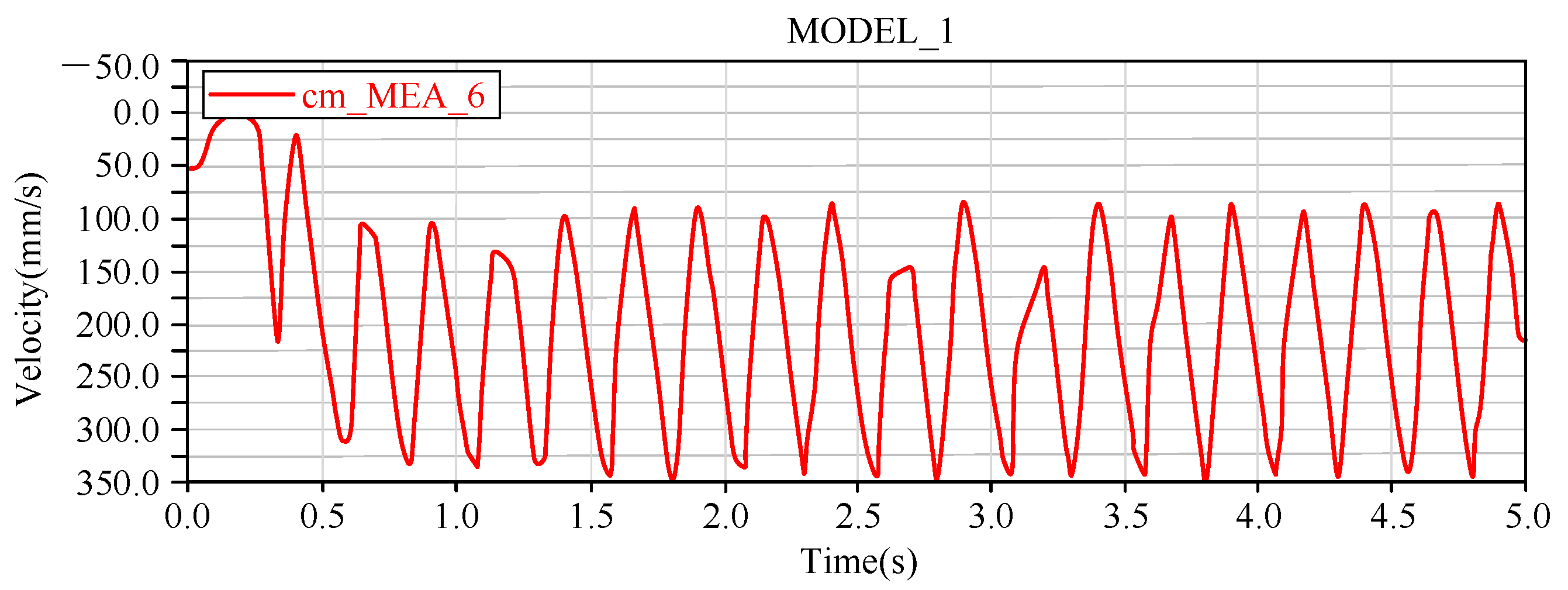
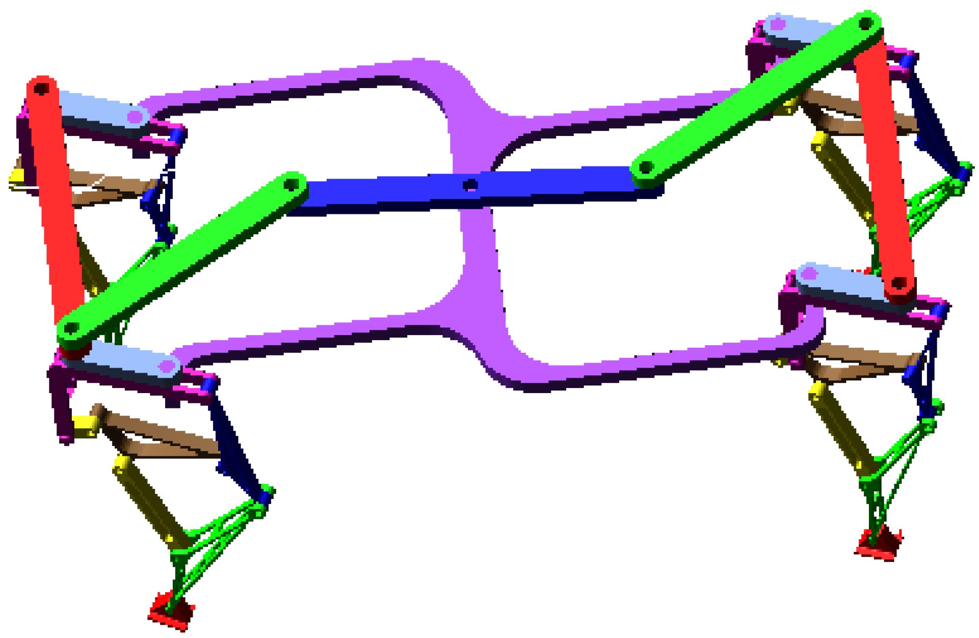
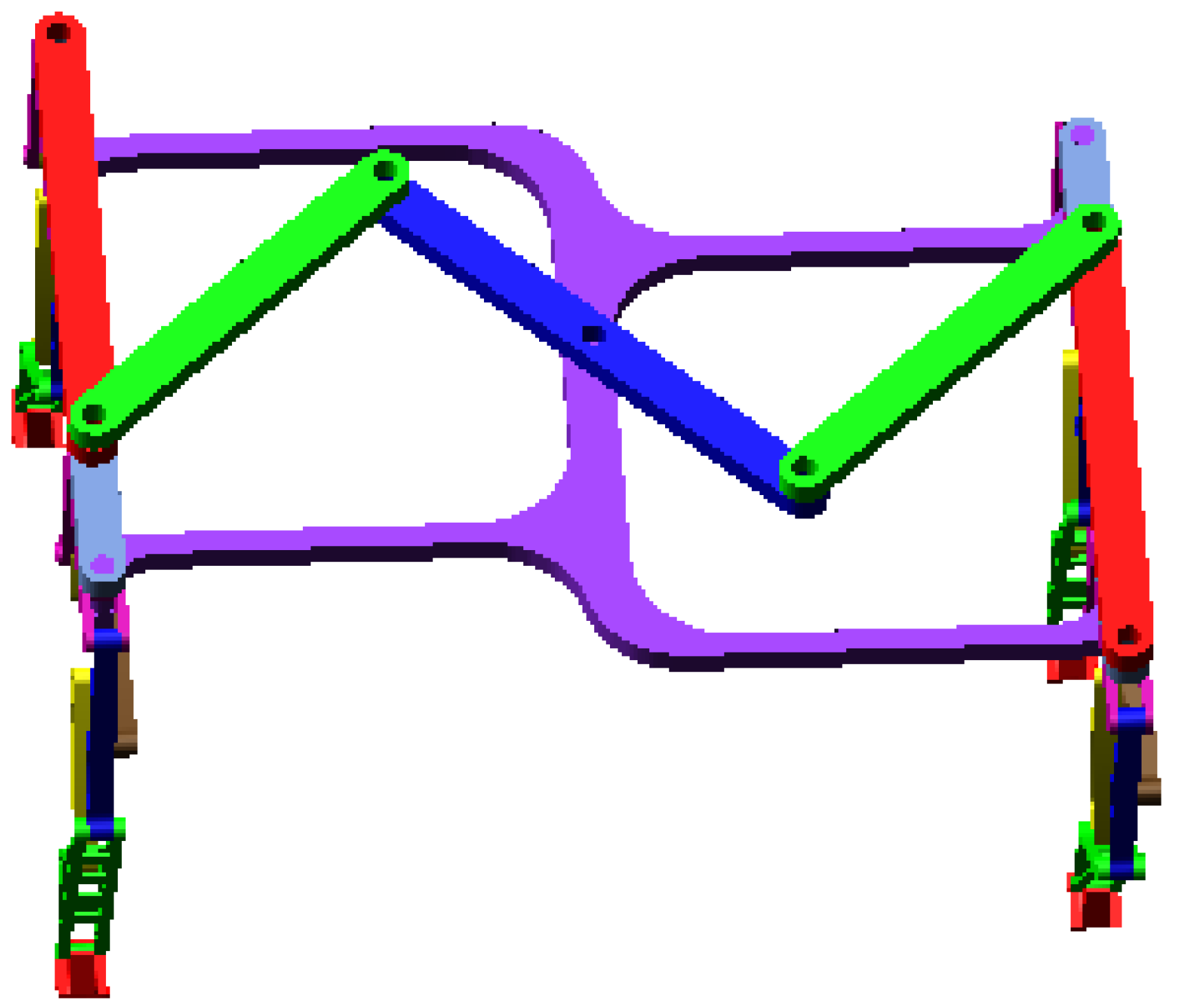
5. Motion Simulation Analysis

5.1. Simulation of Normal Walking Motion

In order to enable the robot to move forward quickly, there must be a certain amount of time to allow the end of the foot to touch down. Therefore, it is necessary to draw the curve of the leg end. Using the designed three-dimensional structure of the closed-chain leg, the ADAMS 2017 software is adopted for simulation and analysis. The trajectory of the single leg of the foot robot is shown in Figure 17. It can be seen from the foot trajectory image that its shape is approximately elliptical, which is essentially consistent with the foot trajectory drawn in MATLAB 2019a in the previous theoretical analysis. For the approximately elliptical trajectory, if we wish to optimize the walking speed, we need to install the semi-major axis parallel to the ground, i.e., in the direction of the arrow in Figure 15. If we wish to raise the leg height, we must install it at an inclined angle. These two installation methods need to be weighed according to the actual requirements.

In this installation situation, the vertical displacement curve of the leg lift height is drawn, as shown in Figure 18. The range of leg lifting is 0–21 mm. If different requirements need to be met, the whole robot can be processed by enlarging or reducing the scale. Since this robot is a four-legged mobile robot, it will inevitably produce centroid fluctuations. Through analysis in the ADAMS 2017 software, the centroid fluctuation changes at a certain point on the robot’s motion platform during the movement are drawn, as shown in Figure 19.

Then, the change curve of the center of mass is drawn, as shown in Figure 20. From the figure, it can be seen that the center of mass of a certain point on the moving platform exhibits periodic changes over time in the vertical direction, and its fluctuation amplitude is 7 mm, which is one-third of the height of the leg lift. When the robot starts, its center of mass fluctuates within a large range, which is consistent with the actual situation.

The height of the four-legged robot is 290 mm, and the driving speed is set to 2 r/s. The friction coefficient will be different when the foot encounters different ground environments. Herein, the friction coefficient is assumed to be 0.3, and the overall walking speed of the robot is simulated. The simulation speed curve is shown in Figure 21.

5.2. Steering Motion Simulation

Focusing on the designed mobile foot robot, its steering movement is analyzed. Before turning, its walking state is as shown in Figure 22.

After advancing a certain distance, the closed-chain leg mechanism begins to turn. In the process of steering, the motion state is as shown in Figure 23.

According to the rotation angle of the driving rod, the foot-type mobile robot can realize steering as a whole, and its motion state is as shown in Figure 24.

To summarize, it is possible to theoretically simulate the various motions of the designed foot-type mobile robot through software modeling, which can realize the motion state analysis of the mechanism under different conditions. Furthermore, we can intuitively analyze the movement of the foot end, providing conditions for the installation and optimization of the foot-end trajectory. The walking stability of the robot is one of the most important indices in the design process, and the stability of the robot’s motion can be analyzed by observing the fluctuations of the drawn center of the robot’s mass. At the same time, the software can clearly analyze the robot’s walking speed corresponding to the prime mover at a certain speed, which is helpful for the selection of the motor and the optimization of the dimensions of the robot.

6. Conclusions

Inspired by the WATT-I leg structure, this study proposes a novel closed-chain foot robot that can move in all directions. The conclusions are summarized as follows. (1) The kinematics and singularity analyses of the robot’s leg structure are carried out, and a three-dimensional model is drawn. After comparing the use of three optimization algorithms for the structural parameters, it can be concluded that the heuristic algorithm used to solve the trajectory reversal problem is far superior to the traditional algorithm. (2) A leg steering mechanism is proposed, and its kinematics and singularity analyses are developed in detail. The analysis results indicate that adding a spring return device can effectively solve the singularities in the configuration of the steering mechanism. (3) An Adams model of the proposed mobile foot robot is established to simulate the trajectories of the moving state and the turning state. The simulation results reflect not only the trajectories of the moving state and the turning state but also the fluctuations of the platform, providing theoretical guidance for the structural dimension optimization of the robot and its application in several practical situations—for example, in the rescue, exploration, or military fields.

References

1. Bekker, M.G. Off-the-road locomotion. In Research and Development in Terramechanics; University of Michigan Press: Ann Arbor, MI, USA, 1960. [Google Scholar]
2. Patel, N.; Scott, G.; Ellery, A. Application of Bekker theory for planetary exploration through wheeled, tracked, and legged vehicle locomotion. In Proceedings of the Space 2004 Conference and Exhibit, San Diego, CA, USA, 30 September 2004; p. 6091. [Google Scholar]
3. Zong, C.; Ji, Z.; Yu, J.; Yu, H. An angle-changeable tracked robot with human–robot interaction in unstructured environments. Assem. Autom. 2020, 40, 565–575. [Google Scholar] [CrossRef]
4. Liu, P.; Huang, K.; Chen, C. Design and Motion Simulation of a New Leg-Wheel Robot. In Proceedings of the 2020 Chinese Automation Congress (CAC 2020), Shanghai, China, 6–8 November 2020. [Google Scholar] [CrossRef]
5. Chu, H.; Qi, B.; Qiu, X.; Zhou, Y. 6-DOF wheeled parallel robot and its automatic type synthesis method. Mech. Mach. Theory 2022, 169, 104646. [Google Scholar] [CrossRef]
6. Liu, J.; Zhao, X.; Tan, M. Legged robots: A review. Robot 2006, 28, 81–88. [Google Scholar]
7. Tan, M.; Wang, S. Research progress on robotics. Acta Autom. Sin. 2013, 39, 963–972. [Google Scholar] [CrossRef]
8. García Armada, E.; Jiménez Ruiz, M.A.; González de Santos, P.; Armada, M. The Evolution of Robotics Research: From Industrial Robotics to Field and Service Robotics; Institute of Electrical and Electronics Engineers: Piscataway, NJ, USA, 2007; Number 1; pp. 90–103. [Google Scholar]
9. Catalano, M.G.; Pollayil, M.J.; Grioli, G.; Valsecchi, G.; Kolvenbach, H.; Hutter, M.; Bicchi, A.; Garabini, M. Adaptive Feet for Quadrupedal Walkers. IEEE Trans. Robot. 2022, 38, 302–316. [Google Scholar] [CrossRef]
10. Fu, Q.; Guan, Y.; Liu, S.; Zhu, H. A Novel Modular Wheel-legged Mobile Robot with High Mobility. In Proceedings of the 2021 IEEE International Conference on Robotics and Biomimetics (IEEE-ROBIO 2021), Sanya, China, 27–31 December 2021; pp. 577–582. [Google Scholar] [CrossRef]
11. Li, L.; Fang, Y.; Yao, J.; Wang, L. Type synthesis of a family of novel parallel leg mechanisms driven by a 3-DOF drive system. Mech. Mach. Theory 2022, 167, 104572. [Google Scholar] [CrossRef]
12. Zang, L.; Yang, S.; Wu, C.; Wang, X.; Teng, F. Design and kinematics analysis of coordinated variable wheel-track walking mechanism. Int. J. Adv. Robot. Syst. 2020, 17, 1729881420930577. [Google Scholar] [CrossRef]
13. Desai, S.G.; Annigeri, A.R.; TimmanaGouda, A. Analysis of a new single degree-of-freedom eight link leg mechanism for walking machine. Mech. Mach. Theory 2019, 140, 747–764. [Google Scholar] [CrossRef]
14. Miler, D.; Birt, D.; Hoic, M. Multi-Objective Optimization of the Chebyshev Lambda Mechanism. Stroj.-Vestn.-J. Mech. Eng. 2022, 68, 725–734. [Google Scholar] [CrossRef]
15. Alizade, R.I.; Kiper, G.; Bagdadioglu, B.; Dede, M.I.C. Function synthesis of Bennett 6R mechanisms using Chebyshev approximation. Mech. Mach. Theory 2014, 81, 62–78. [Google Scholar] [CrossRef]
16. Nansai, S.; Elara, M.R.; Iwase, M. Dynamic Analysis and Modeling of Jansen Mechanism. In Proceedings of the International Conference on Design and Manufacturing (ICONDM2013), Chennai, India, 18–20 July 2013; Volume 64, pp. 1562–1571. [Google Scholar] [CrossRef]
17. Patnaik, L.; Umanand, L. Kinematics and dynamics of Jansen leg mechanism: A bond graph approach. Simul. Model. Pract. Theory 2016, 60, 160–169. [Google Scholar] [CrossRef]
18. Singh, R.; Bera, T.K. Walking Model of Jansen Mechanism-Based Quadruped Robot and Application to Obstacle Avoidance. Arab. J. Sci. Eng. 2020, 45, 653–664. [Google Scholar] [CrossRef]
19. Sheba, J.K.; Elara, M.R.; Martinez-Garcia, E.; Tan-Phuc, L. Design and Evaluation of Reconfigurable Klann Mechanism based Four Legged Walking Robot. In Proceedings of the 2015 10th International Conference on Information, Communications and Signal Processing (ICICS), Singapore, 2–4 December 2015. [Google Scholar]
20. Komoda, K.; Wagatsuma, H. Energy-efficacy comparisons and multibody dynamics analyses of legged robots with different closed-loop mechanisms. Multibody Syst. Dyn. 2017, 40, 123–153. [Google Scholar] [CrossRef]
21. Rafeeq, M.; Toha, S.F.; Ahmad, S.; Yusof, M.S.M.; Razib, M.A.M.; Bahrin, M.I.H.S. Design and Modeling of Klann Mechanism-Based Paired Four Legged Amphibious Robot. IEEE Access 2021, 9, 166436–166445. [Google Scholar] [CrossRef]
22. Li, T.; Ceccarelli, M. Design and simulated characteristics of a new biped mechanism. Robotica 2015, 33, 1568–1588. [Google Scholar] [CrossRef]
23. Baskar, A.; Plecnik, M.; Hauenstein, J.D. Finding straight line generators through the approximate synthesis of symmetric four-bar coupler curves. Mech. Mach. Theory 2023, 188, 105310. [Google Scholar] [CrossRef]
24. Yin, L.; Huang, L.; Huang, J.; Xu, P.; Peng, X.; Zhang, P. Synthesis Theory and Optimum Design of Four-bar Linkage with Given Angle Parameters. Mech. Sci. 2019, 10, 545–552. [Google Scholar] [CrossRef]
25. Jaiswal, A.; Jawale, H.P. Comparative study of four-bar hyperbolic function generation mechanism with four and five accuracy points. Arch. Appl. Mech. 2017, 87, 2037–2054. [Google Scholar] [CrossRef]
26. Bai, S.; Angeles, J. Coupler-curve synthesis of four-bar linkages via a novel formulation. Mech. Mach. Theory 2015, 94, 177–187. [Google Scholar] [CrossRef]
27. Ivolga, D.V.; Borisov, I.I.; Nasonov, K.V.; Kolyubin, S.A. Computational Design of Closed-Chain Linkages: Respawn Algorithm for Generative Design. In Proceedings of the 2023 IEEE/RSJ International Conference on Intelligent Robots Furthermore, Systems, (IROS), Detroit, MI, USA, 1–5 October 2023; pp. 481–486. [Google Scholar] [CrossRef]
28. Tole, G.; Williams, G.; Holland, A.E.; Clark, R.A. Lower limb muscle performance during a closed chain single leg squat and a squat jump in people with leg weakness after stroke: A comparative study. Brain Impair. 2022, 25, IB22031. [Google Scholar] [CrossRef]
29. Liu, G.; Trinkle, J.; Yang, Y.; Luo, S. Motion Planning of Planar Closed Chains Based on Structural Sets. IEEE Access 2020, 8, 117203–117217. [Google Scholar] [CrossRef]
30. Shafei, A.M.; Shafei, H.R. Dynamic modeling of planar closed-chain robotic manipulators in flight and impact phases. Mech. Mach. Theory 2018, 126, 141–154. [Google Scholar] [CrossRef]
31. Wu, J.; Yao, Y.A. Design and analysis of a novel walking vehicle based on leg mechanism with variable topologies. Mech. Mach. Theory 2018, 128, 663–681. [Google Scholar] [CrossRef]
32. Wu, J.; Yao, Y.; Ruan, Q.; Liu, X. Design and optimization of a dual quadruped vehicle based on whole close-chain mechanism. Proc. Inst. Mech. Eng. Part-J. Mech. Eng. Sci. 2017, 231, 3601–3613. [Google Scholar] [CrossRef]
33. Yan, H.; Yao, Y. Creative Design of Mechanical Devices; China Machine Press: Beijing, China, 2002. [Google Scholar]
34. Huang, Z.; Zhao, Y.S.; Zhao, T.S. Advanced Spatial Mechanism; China Higher Education Press: Beijing, China, 2006; pp. 89–201. [Google Scholar]
35. Gu, R. Optimal design of planar four-bar mechanism with trajectory representation. J. Nantong Vocat. Univ. 2011, 25, 97–100. [Google Scholar]
36. Wu, J. The Design and Application of the Link Type Integral Closed Chain Multi Sufficient Transportation Platform; Beijing Jiaotong University: Beijing, China, 2019. [Google Scholar]
37. Li, P.; Peng, S.; Che, L.; Du, L.; Wu, Z. Application of hybrid artificial bee colony algorithm in scale optimization of parallel mechanism. Mech. Des. 2019, 36, 90–96. [Google Scholar]
Figure 1. Creative design methodology for mechanical devices.
Applsci 14 06805 g001
Figure 2. Single-leg mechanical structure.
Applsci 14 06805 g002
Figure 3. Coordinate system of closed-chain single-leg mechanism.
Applsci 14 06805 g003
Figure 4. Establishing the leg coordinate system.
Applsci 14 06805 g004
Figure 5. Schematic diagram of institutional parameters.
Applsci 14 06805 g005
Figure 6. Preset trajectory diagram.
Applsci 14 06805 g006
Figure 7. The relationship between the number of iterations and the individual fitness.
Applsci 14 06805 g007
Figure 8. Foot trajectory curve obtained with calculated values.
Applsci 14 06805 g008
Figure 9. Structure 1.
Applsci 14 06805 g009
Figure 10. Structure 2.
Applsci 14 06805 g010
Figure 11. Parallelogram mechanism.
Applsci 14 06805 g011
Figure 12. Layout of four closed-chain single-leg mechanisms.
Applsci 14 06805 g012
Figure 13. Overall structure.
Applsci 14 06805 g013
Figure 14. Movement diagram of steering mechanism.
Applsci 14 06805 g014
Figure 15. Steering mechanism.
Applsci 14 06805 g015
Figure 16. Establishing coordinate system of the parallelogram structure mechanism.
Applsci 14 06805 g016
Figure 17. Foot trajectory.
Applsci 14 06805 g017
Figure 18. Changes in height displacement of leg lift.
Applsci 14 06805 g018
Figure 19. The fluctuation curve of a point on the motion platform.
Applsci 14 06805 g019
Figure 20. Centroid change curve.
Applsci 14 06805 g020
Figure 21. Overall walking speed curve.
Applsci 14 06805 g021
Figure 22. Movement state before turning.
Applsci 14 06805 g022
Figure 23. Movement state during steering.
Applsci 14 06805 g023
Figure 24. Movement state after steering.
Applsci 14 06805 g024