Frequency Coordination Control Strategy for Large-Scale Wind Power Transmission Systems Based on Hybrid DC Transmission Technology with Deep Q Network Assistance

Abstract

Wind power is currently the most mature representative of sustainable energy generation technology, which has been developed and utilized on a large scale worldwide. The random and fluctuating nature of wind power output poses a threat to the secure and stable operation of the system. Consequently, the transmission of wind power has garnered considerable attention as a crucial factor in mitigating the challenges associated with wind power integration. In this paper, an artificial-intelligence-aided frequency coordination control strategy applicable to wind power transmission systems based on hybrid DC transmission technology is proposed. The line commutated converter (LCC) station at the sending end implements the strategy of auxiliary frequency control (AFC) and automatic generation control (AGC) to cooperate with each other in order to assist the system frequency regulation. The AFC controller is designed based on the variable forgetting factor recursive least squares (VFF-RLS) algorithm for system identification. First, the VFF-RLS algorithm is used to identify the open-loop transfer function of the system. Then, the AFC controller is designed based on the root locus method to achieve precise control of the system frequency. The DC line power modulation quantity is introduced in the AGC to automatically track the active power fluctuation and frequency deviation of the system. The AGC utilizes the classical proportional-integral (PI) control. By selecting the integrated time absolute error (ITAE) performance index to construct the reward function, and using a deep Q-network (DQN) for controller parameter optimization, it achieves improved regulation performance for the AGC. The voltage source converter (VSC) station at the receiving end implements an adaptive DC voltage droop control (ADC)strategy. Finally, the effectiveness and robustness of the proposed frequency control strategy are verified through simulation experiments.

1. Introduction

Wind energy is currently the fastest growing and most commercially promising clean renewable energy source globally. With its mature technology and low-cost advantage, wind power generation has been developed and utilized on a large scale, demonstrating high environmental, economic, and social benefits [1,2]. Due to the long-distance, high-capacity transmission capabilities far exceeding those of AC transmission, along with flexible control and lower loss, DC transmission has become the primary method for the large-scale transmission of wind power.

However, due to the weak AC grid infrastructure and the singular power structure in wind power regions, it is necessary to integrate a certain capacity of hydropower or thermal power units to meet the power fluctuations of wind power. In [3], a cost-effective off-grid power system for clean energy generation consisting of wind energy, pumped storage and open wells was proposed. Reference [4] established a simulation model of a water–wind complementary operation system and investigated the dynamic response characteristics of this system under active power control.

According to the different converters of the transmission line, there exist two types of DC wind power transmission: LCC-HVDC and VSC-HVDC. In comparison with traditional DC transmission technologies, the flexible DC transmission based on VSC has no reactive power compensation problem and no commutation faults [5,6,7]. Flexible DC transmission has become a hot topic of research, and several studies have explored ways to further enhance the performance of VSC-HVDC systems. Reference [8] constructed a hybrid AC-DC system including a VSC-MTDC system, onshore grids, and offshore wind farms. An adaptive droop control strategy was proposed. It mentioned that converter stations can autonomously adjust their DC voltage reference based on grid frequency deviation, allowing for the redistribution of power. The performance of the ADC strategy was verified, which can enhance the system’s response to frequency fluctuations. This provides a new approach for efficient control of power systems.

Wind power, with its intermittent and highly stochastic characteristics, can lead to large fluctuations in output power when integrated into the system on a large scale, significantly impacting the frequency based on the active power balance [9]. Reference [10] investigates the frequency stability concerns arising from the integration of large-scale wind power into the system. The findings suggested that conventional power system frequency control methods are no longer adequate to meet the heightened demands posed by the frequent and substantial fluctuations in wind power output for maintaining power system frequency stability. Moreover, in the case of large-scale wind power grid integration, the uncertainty of wind power significantly increases the adjustment pressure on AGC units, which makes the regulation performance of AGC on system power and frequency fluctuations worse [11].

PI control is a traditional method widely used in AGC systems. In the field of industrial control, various techniques have been applied to tune the parameters of PID controllers. Traditional PI control often faces challenges in selecting parameters that yield optimal performance. To address this, recent studies have incorporated artificial intelligence (AI) techniques for PID controller tuning to achieve better performance. The three main branches of AI are neural networks, fuzzy control, and genetic algorithms, which can be integrated with the PID controller, respectively [12]. Reference [13] focused on an air rudder servo system and proposed a PI control method optimized by a genetic algorithm. The genetic algorithm optimized the initial parameters of the PI controller, and the deep deterministic policy gradient algorithm controller performs real-time tuning. However, this type of controller is often used for offline parameter tuning and has poor real-time performance. Reference [14] addressed the issue of voltage tracking control for inverters under load disturbances and input–output constraints. Based on the time-domain mathematical model of voltage and current in the synchronous rotating coordinate system, it proposed a constraint adaptive PI control strategy based on neural networks. In terms of artificial intelligence involvement in control strategies, ref. [15] constructed a deep learning model for AGC strategy using long short-term memory (LSTM) recurrent neural networks as neurons, and it proposed a data-driven AGC real-time control strategy based on LSTM recurrent neural networks. Additionally, ref. [16] proposed a frequency control strategy for islanded microgrids based on DQN to address the issue of frequency control when microgrids are subjected to strong random disturbances and changes in network topology parameters. Deep reinforcement learning (DRL) integrates deep learning with reinforcement learning, enabling the autonomous learning of optimal strategies through environmental interaction in unknown settings, thus eliminating the need for extensive manual feature engineering or rule design. Currently, several notable applications of DRL have been developed. For instance, ref. [17] employs DRL to propose an automatic power flow adjustment application that considers static stability constraints. This method effectively measures the sensitivity of each device’s adjustment to changes in system power flow, thereby accelerating the convergence speed of power flow. Additionally, ref. [18] introduces an optimal configuration strategy for system measurement devices based on observability strength and proposes a GCN-DDPG algorithm to ensure system observability across multiple scenarios. Moreover, some researchers have applied DRL to achieve automatic generation control (AGC).

Considering that DC modulation has been widely used to improve the frequency stability of the system, while meeting the basic requirements for large-scale conventional energy and wind power transmission, making full use of the fast controllability of DC transmission power in order to coordinate the active power control can improve the stability of the wind power delivery, as well as greatly improving the utilization rate of the DC transmission system and the capacity of wind power transmission [19,20,21]. To enhance the frequency response capability of high-proportion wind power electrical systems and maintain system frequency stability, research on how wind power participates in system frequency regulation mainly focuses on using additional control of wind turbine generators to respond to changes in system frequency [22]. In [23], an enhanced strategy for HVDC transmission to engage in auxiliary frequency control was introduced and experimentally validated, and the results indicated that employing HVDC instead of relying on wind power frequency regulation reserves can significantly improve system frequency stability. Reference [24] focused on improving the poor system stability when constant voltage and frequency (V/F) control was used for a direct-drive wind farm side converter station via a flexible DC transmission system.

Considering the LCC-VSC hybrid DC transmission system, this paper proposes a frequency coordination control strategy applicable to wind power transmission systems based on hybrid DC transmission technology. Finally, simulations are conducted using PSCAD/EMTDC, and the feasibility and effectiveness of the control strategy are validated by comparing with the system response without AFC.

The specific innovative contributions are as follows:

For the sending end, an additional frequency controller is designed based on the VFF-RLS algorithm and root locus method. It is proposed to use AFC in coordination with AGC using conventional PI control to suppress frequency fluctuations caused by changes in wind power output. Additionally, to achieve better control performance of the AGC, artificial intelligence with deep Q-network (DQN) assistance is introduced to optimize the PI parameters of the AGC.

For the receiving end, an adaptive DC voltage droop control method is proposed. This method allows the droop coefficient to adapt to changes in DC power and voltage, thereby reasonably distributing unbalanced power and improving the responsiveness of power adjustments at the converter station.

2. Hybrid DC Transmission System

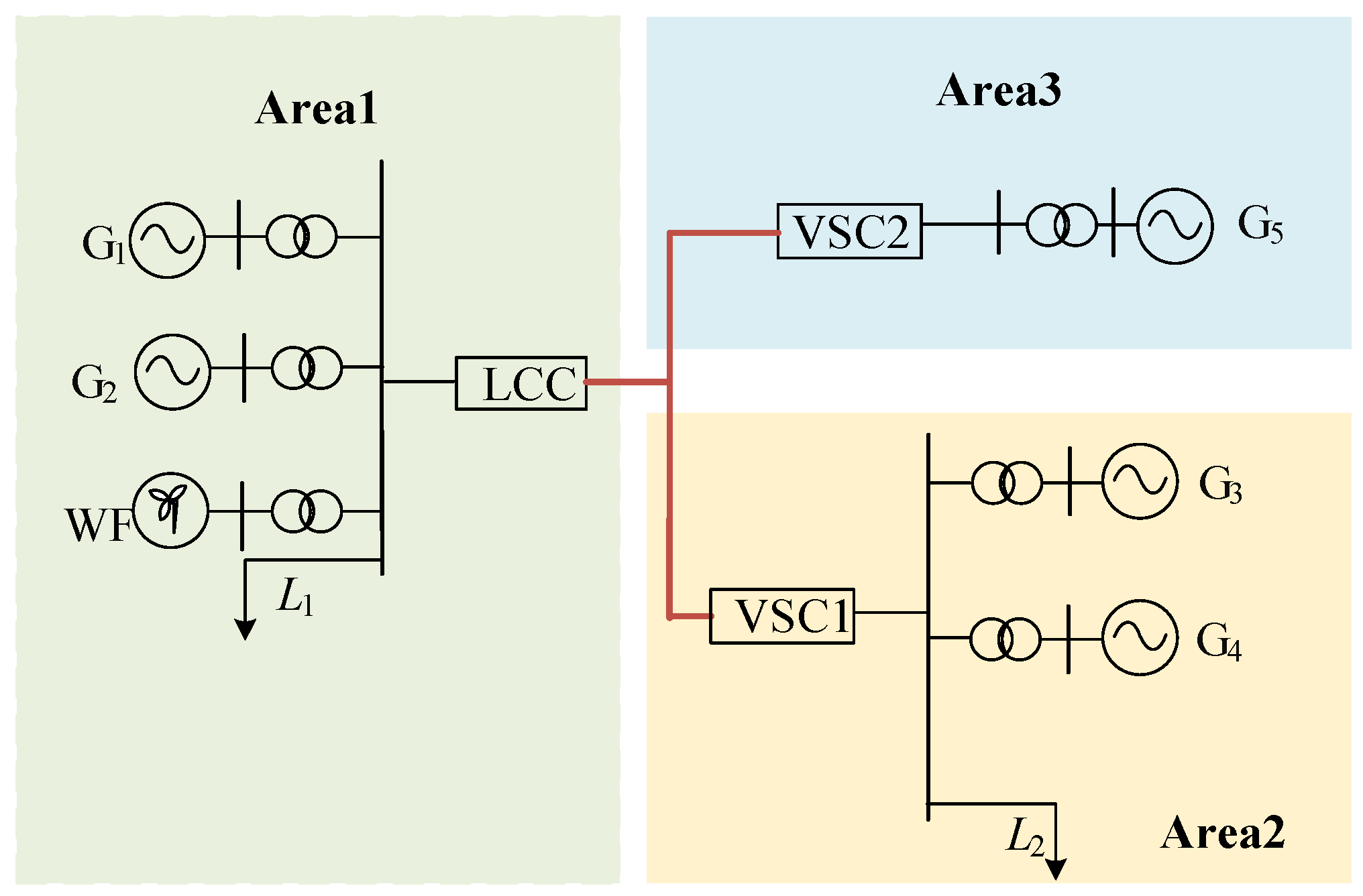
2.1. Structure of the Hybrid DC Transmission System

For large-scale and long-distance transmission from wind power bases that are more than 1000 km away from the load center, LCC-HVDC is still a more appropriate choice. However, this method has defects, such as the risk of commutation failure and more loss in reactive power. In contrast, VSC-HVDC transmission not only avoids the problem of commutation failure but also realizes independent and rapid control of active and reactive power. Additionally, the transmission line possesses a certain capacity for reactive support, allowing for the dynamic compensation of reactive power in the AC system.

To fully exploit the high voltage and large capacity transmission capability of the LCC converter station and the flexible control of the VSC converter station, a hybrid LCC-VSC DC transmission system is considered [25]. Through appropriate control strategies, power coordination control is achieved to mitigate the impact of wind power fluctuations on system stability. The four-machine, two-area model is used as the basis [26] in which the VSC-MTDC system is embedded, and the wind farm is connected in Area 1, where G1 and G2 are hydroelectric units. The wind power units in Area 1 are connected to the same AC bus as the hydroelectric units in the local grid, and active power is transmitted to Areas 2 and 3 through DC lines.

The wind farms are equipped with a certain percentage of hydroelectric turbine FM capacity to smooth out fluctuations in wind power output. As shown in Figure 1.

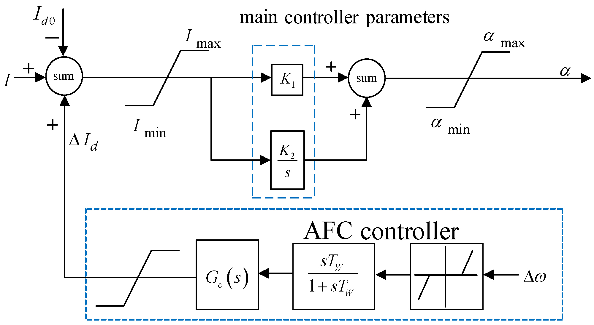
2.2. Control Strategies of the Hybrid DC Transmission System

When the system integrates large-scale wind power, the significant and frequent fluctuations in wind power pose stricter requirements for power system frequency control. Traditional frequency control methods are currently insufficient to meet the demands of safe and stable system operation. While wind–hydro bundling alleviates wind power fluctuations to some extent, the adjustment speed of hydroelectric units cannot promptly follow the changes in wind power output, leading to potential power fluctuations. Therefore, considering the fast controllability of DC power, the stability of the wind power integration system can be improved, fully exploiting the modulation characteristics of DC transmission systems.

Conventional frequency control primarily relies on governor response to achieve the absorption of wind power imbalance increments, but the capacity for adjustment is quite limited. Therefore, according to the operating conditions and characteristics of the system, when the hybrid LCC-VSC DC system is applied to wind power transmission, in order to ensure the stable operation of the transmission system, the LCC station is set up to use the control strategy of AFC and AGC to coordinate and cooperate so that the AGC unit G1 balances most of the incremental wind power, and the AFC modulates the DC active power in order to balance the small-amplitude and short-period active power disturbance components to assist the primary frequency regulation.

At the same time, the DC transmission line power modulation is introduced into the AGC to coordinate with the AFC to track the active power fluctuation and frequency deviation of the system automatically, and the AGC unit active output is adjusted to balance the active power disturbance component with a large amplitude and a long period and ultimately to realize the difference-free regulation of the frequency. VSC2 and VSC3 stations use an adaptive DC voltage droop control to adapt to the frequent changes in wind farm currents and to guarantee the stability of the DC voltage of the receiving end system.

3. Frequency Coordination Control Strategy at LCC Terminal

3.1. Auxiliary Frequency Controller Design Based on VFF-RLS Algorithm

Auxiliary frequency controllers can be used to assist in the primary frequency regulation of power systems, with the basic principle being DC active power modulation. The deviation in active power caused by the small-amplitude, short-period, and rapidly changing wind power output fluctuations is denoted as ΔP. This is equivalent to a load disturbance with the same amplitude and period, and the frequency deviation caused by this disturbance is considered as primary frequency control, adjusted by the governor of the generator unit. Therefore, according to the power balance relation, it is expressed as follows:

$$\Delta P=\Delta P_G-\Delta P_D=K\Delta f,$$

(1)

where ΔP_G represents the power increment adjusted by the generator unit based on the droop characteristic, and ΔP_D represents the load increment adjusted by the load regulation effect. K is the power–frequency static characteristic coefficient. From (1), the larger the value of K, the smaller the frequency variation caused by power fluctuations in the system. Therefore, the stability of the system frequency can be improved.

The AFC controller achieves power regulation by adding a DC current modulation signal to the main controller of the LCC converter station; the specific structure is shown in Figure 2, where Δω represents the selected speed difference between generators, T_w is the time constant of the DC-blocking link, G_c(s) is the controller transfer function, ΔI_d is the DC current regulation command, I is the actual measurement of DC current, I_d0 is the DC current setpoint, K₁ and K₂ are parameters of the LCC converter station main controller, and α represents the firing angle.

The specific principle of the AFC controller is summarized as follows:

When the system frequency fluctuation exceeds the action frequency set by the AFC controller, the AFC controller responds and outputs an additional DC current regulation command ΔI_d, which is superimposed on the main controller of the LCC converter station, jointly participating in modulating the active power of the DC interconnection line. The rapid increase or decrease in active power in the DC contact line is utilized to alleviate the active power imbalance in the area and to realize the mutual support of power between areas, thus improving the system frequency.

The additional DC current regulation command ΔI_d is output by the AFC controller, which can be used to obtain the additional DC power regulation command ΔP_dc to regulate the DC power. K_dc is the corresponding frequency regulation coefficient The Equation (1) can be rewritten as follows:

$$\Delta P=\Delta P_G-\Delta P_D+\Delta P_{\mathrm{dc}}=(K+K_{\mathrm{dc}})\Delta f.$$

(2)

From (1) and (2), it can be seen that the participation of AFC is equivalent to improving the active power–frequency static characteristic coefficient of the system; that is to say, for the same amount of power variation, the system with AFC participation has a small amount of frequency variation. Thus, the stability of the system frequency is enhanced. To avoid frequent responses of the AFC controller to the active power of the DC line, a dead zone limit link is introduced, and the size of the dead zone limit needs to be coordinated with the primary frequency modulation. In addition, to eliminate the influence of steady-state error on the controller, a time constant Tw = 10 s is added after the dead zone limit link.

The recursive least squares (RLS) algorithm is an adaptive filtering algorithm commonly used for system identification. The basic idea is to transform the system model, minimizing the sum of squared errors and performing recursive operations on the instantaneous input data to find the optimal parameters. This overcomes the limitations of offline identification and enables the online identification of parameters.

The forgetting factor λ is one of the key parameters in RLS algorithm, and the convergence speed, tracking speed, and correction effect of the algorithm are all affected by the forgetting factor. VFF-RLS algorithm is adopted to make the forgetting factor dynamically adjusted according to the changes of the estimated parameters so as to realize a faster tracking speed, have a small parameter estimation error, and improve the online recognition accuracy. The defining expression is as follows:

$$\lambda \left(k\right)={\lambda }_{\max }-\left({\lambda }_{\max }-{\lambda }_{\min }\right)\times \tan \mathrm{h}\left(\mu \times {\displaystyle \sum }_{j=0}^M\parallel \mathrm{e}\left(k-j\right){\parallel }^2\right),$$

(3)

where λ_max and λ_min is the range of the forgetting factor adjustment to ensure that RLS algorithm does not diverge during iteration. The error e comes from the error between the calculated value and the real measured value, reflecting the dynamic changes in parameters by calculating the error.

The approach to realize the identification of the open-loop transfer function of the system is as follows:

Utilizing the low-amplitude step disturbance at the control signal of the rectifier-side main controller as the input I, the inter-generator speed difference is used as output y_. Assuming the sensor sampling error at time k is e(k), then

$$y\left(k\right)={\mathsf{\Phi }}^T\left(k\right)\theta +e\left(k\right).$$

(4)

To minimize the sum of squares of the errors between the estimate of ${\widehat{y}}_k={\mathsf{\Phi }}_k\widehat{\theta }$ and the actual value of $y_k={\mathsf{\Phi }}_k\widehat{\theta }$, minimize $J\left(\widehat{\theta }\right)={(y-\mathsf{\Phi }\widehat{\theta })}^T\left(y-\mathsf{\Phi }\widehat{\theta }\right)$.

Let

$${\left.{\displaystyle \frac{\partial J}{\partial \theta }}\right|}_{\theta =\widehat{\theta }}=-2{\mathsf{\Phi }}^T\left(y-\mathsf{\Phi }\widehat{\theta }\right)=0,$$

(5)

resulting in

$$\widehat{\theta }={\left({\mathsf{\Phi }}^T\mathsf{\Phi }\right)}^{-1}{\mathsf{\Phi }}^{T}y.$$

(6)

Each time the system updates the measurement data each time, it will update the matrix Φ and the I_k matrix, thereby further correcting the existing estimated values. Consequently, as the system continually updates the measurement data, the identified parameters also continuously evolve.

The steps of the VFF-RLS algorithm are as shown in

Table 1. Steps of the VFF-RLS algorithm.

Serial Number	Steps and Instructions
1	Input Parameters	${\theta }_0,P_0,{\lambda }_0,I_k,U_k$
2	Update Gain Matrix	$K_k=P_{k-1}{\mathsf{\Phi }}_k{ }^T{\left[\lambda +{\mathsf{\Phi }}_k{P}_{k-1}{\mathsf{\Phi }}^T{ }_k\right]}^{-1}$
3	Update Parameters	${\theta }_k={\theta }_{k-1}+K_k\left(y_k-{\mathsf{\Phi }}_k{\theta }_{k-1}\right)$
4	Update Covariance	$P_k={\displaystyle \frac{1}{\lambda }}\left(I-K_k{\mathsf{\Phi }}_k\right)P_{k-1}$
5	Calculate Parameter Error	$e=f\left({\theta }_k\right)-y_k$
6	Update Forgetting Factor	$\lambda \left(k\right)={\lambda }_{\max }-\left({\lambda }_{\max }-{\lambda }_{\min }\right)\times \tan \mathrm{h}\left(\mu \times {\displaystyle {\displaystyle \sum }_{j=0}^M}\parallel \mathrm{e}\left(k-j\right){\parallel }^2\right)$
7	Output Online Identified Parameters	${\theta }_k$

.

In order to realize the precise control of the system frequency, the root locus method is used to design the AFC controller. The root locus method is a graphical method which is easy to implement, and it has been widely used in engineering practice. The position of the closed-loop pole determines the stability and dynamic characteristics of the system. By adjusting the position of the closed-loop pole, the dynamic performance of the system can be regulated.

The basic principle is to use the open-loop transfer function obtained by using the VFF-RLS algorithm to identify an open-loop system. Based on the root locus of the open-loop system, the dominant poles of the system are determined for the desired dynamic characteristics. Negative feedback correction is applied by adding zeros and poles to the open-loop transfer function through the correction loop G_c(s). This adjustment positions the closed-loop dominant poles of the system at the desired ideal dominant poles, making the closed-loop system’s root locus pass through these characteristic roots for improved system stability and dynamic response characteristics. The control system block diagram is shown in Figure 3. With the addition of the correction section, the system’s open-loop transfer function ϕ₀(s), closed-loop function ϕ(s), and closed-loop characteristic equation are as follows:

$${\varphi }_0(s)=G(s),$$

(7)

$$\varphi (s)={\displaystyle \frac{G(s)}{1+G(s)G_c(s)}},$$

(8)

$$1+G(s)G_c(s)=0.$$

(9)

The root locus curve of the system after correction passes through the ideal dominant pole $s_d=a\pm bi$, which satisfies the phase angle condition and magnitude condition:

$$\left\{\begin{array}{l}{\left.\angle G(s)G_c(s)\right|}_{s=s_d}={\displaystyle \sum _{i=1}^m\angle (s+z_i)}-{\displaystyle \sum _{j=1}^n\angle (s+p_i)}=\pm {180}^{\mathrm{o}}(2k+1)\\ {\left.\left|G(s)G_c(s)\right|\right|}_{s=s_d}=1\end{array}\right.,$$

(10)

where m and n represent the orders of the zeros and poles, while z and p represent the zeros and poles.

$$G_c(s)=K{\displaystyle \frac{s+T_1}{s+T_2}},$$

(11)

where K is determined by the magnitude condition, and T₁ and T₂ are determined by the phase condition. Plugging the dominant pole s_d into the open-loop system transfer function G(s) determines its phase deficiency and open-loop gain deficiency. From (10), the specific parameters of the correction section G_c(s) can be determined, obtaining the transfer function of the auxiliary frequency control.

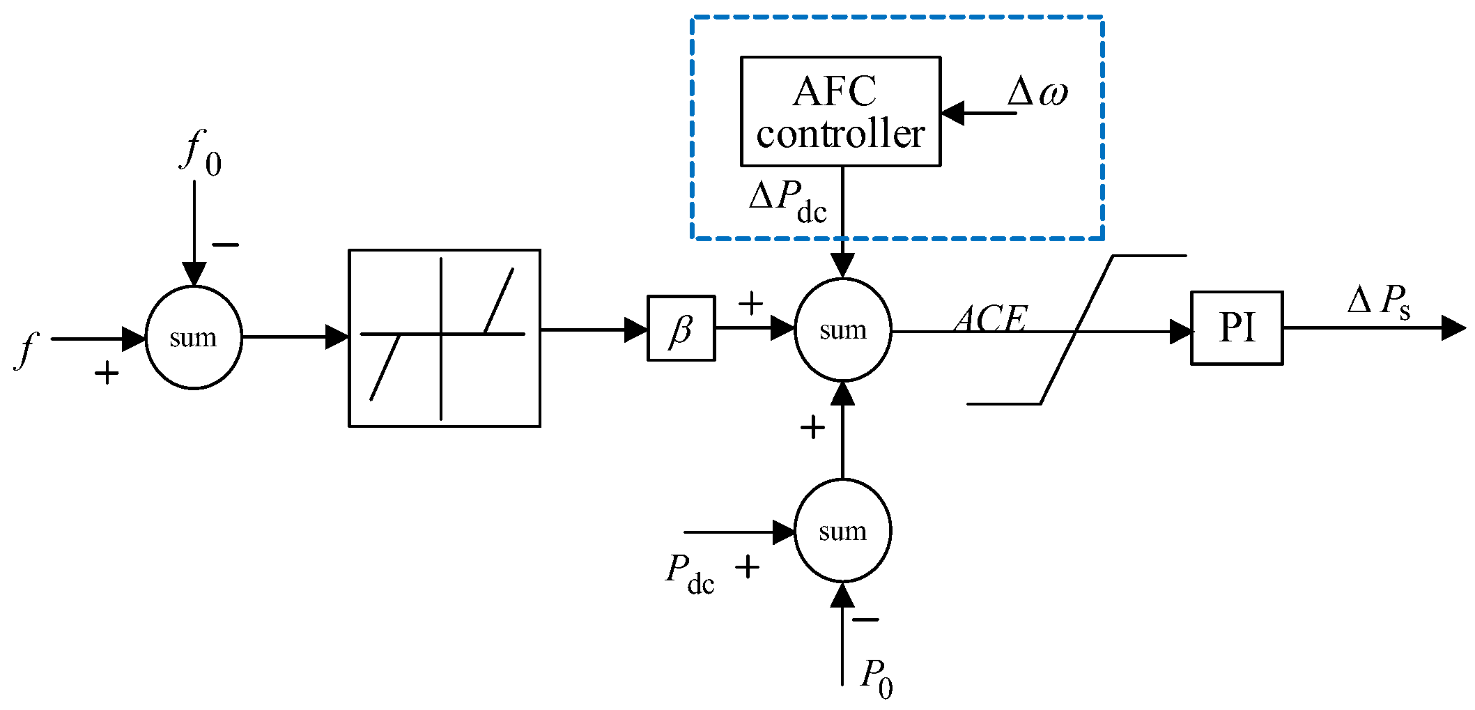
3.2. AGC Controller Parameter Optimization Using DQN Algorithm

The fundamental idea of deep learning (DL) is to transform high-dimensional data into a low-dimensional feature representation through multi-layer neural networks and nonlinear transformations. The fundamental idea of reinforcement learning (RL) is to interact with the environment in real time, learning from experiences in the process of continuous failures and successes, maximizing the cumulative reward obtained by the agent from the environment, and ultimately allowing the agent to learn the optimal strategy. The DQN algorithm effectively integrates deep learning and reinforcement learning, addressing the instability issues associated with using neural networks and other nonlinear function approximators to represent action-value functions. The DQN algorithm is based on Q-learning and uses a neural network model instead of a Q-value table to directly predict Q-function values. The current target Q-value is calculated, and then the neural network parameters are updated using the mean square error between the current target Q-value and the predicted Q-value of the neural network. Since AGC controllers are crucial for maintaining power system stability and operation, the optimization of AGC controller parameters involves a high-dimensional parameter space, which needs to handle the complex dynamic environment. Compared with other optimization algorithms, DQN optimization can handle the high-dimensional state space in many practical problems, and it can adapt to the changes in system dynamics and learn the optimal control strategy under different operating conditions. Therefore, we chose to use the DQN algorithm to optimize the PI parameters of the AGC controller. The core ideas of the DQN algorithm can be summarized in the following three points:

(1)

Loss Function.

Training a neural network essentially involves optimizing a loss function. The lower the loss function, the higher the robustness of the model. The DQN algorithm constructs a learnable loss function based on the Q-learning algorithm. The update formula for the algorithm is shown in Equation (12):

$$Q\left(s,a\right)\leftarrow Q\left(s,a\right)+\mathrm{lr}\left(r+\underset{a\in A}{\max }Q\left(s^{\prime },a\right)-Q\left(s,a\right)\right).$$

(12)

We use the mean squared error between the current Q value and the target Q value to define the loss function of the DQN algorithm, as shown in Equation (13):

$$L\left(\theta \right)=E\left[{\left(r+\gamma \underset{a\in A}{\max }Q\left(s^{\prime },a^{\prime };\theta \right)-Q\left(s,a;\theta \right)\right)}^2\right],$$

(13)

where θ represents the weight parameters of the convolutional neural network model, and γ represents the decay factor, $r+\gamma {\max }_{a\in A}Q\left(s^{\prime },a^{\prime };\theta \right)$, which is the target Q value. After obtaining the loss function, the weight parameters θ of the convolutional neural network can be directly solved using the gradient descent method.

(2)

Experience Replay Mechanism.

The DQN algorithm adopts an experience replay mechanism, storing the experiential data generated by the agent’s interaction with the surrounding environment in an experience pool. During network iteration training, several data points are randomly extracted from the experience pool for model training. Each experiential data are stored in the form of a five-tuple $\left(s,a,r,s^{\prime },T\right)$, where T is a Boolean value used to indicate whether the next state $s^{\prime }$ is a target or terminal state. This can effectively eliminate the correlation between data samples, reduce the error of approximating the value function, and avoid mutual influence between data and non-stationary distribution problems, thereby improving the convergence speed of the network model.

(3)

Dual Network Structure.

DQN adopts two neural networks with identical structures but different parameters, which are called action value estimation network and target value network. By introducing the target network, the correlation between the current Q-value and the target Q-value can be effectively suppressed. It can avoid the difficulty of network convergence during iterative training and greatly improve the convergence speed and stability of the algorithm.

By using DQN, the control parameters of AGC can be optimized. The state space s_t is as follows:

$$s_t=(t,K_P,K_I,\Delta f,\Delta P),$$

(14)

where the state space includes the current period, t, and the PI parameters K_P and K_I of the AGC controller. Δf is the frequency deviation, and ΔP is the active power deviation.

Action space α_t using DQN is as follows:

$$a_t=(\Delta K_P,\Delta K_I).$$

(15)

Since the main task of the AGC is to keep the frequency in the area stable and the active power of the DC line within the planned value after a disturbance, the ITAE performance metrics are selected to construct the reward function r_t, which is as follows:

$$r_t=-{\displaystyle {\int }_0^{T}t\left|\alpha \left|\Delta f\right|+\beta \left|\Delta P_{dc}\right|\right|}dt.$$

(16)

3.3. Frequency Coordination Control through AFC and AGC

The AGC unit responds to the area control error (ACE) signal by outputting reference load adjustment commands to the governor. It adjusts the output of the generator units to maintain the scheduled exchange power P_AB on the tie line while ensuring the stability of system frequency and voltage. The basic control modes of AGC include scheduled tie-line power control, scheduled frequency control, and tie-line frequency deviation control. In this paper, tie-line frequency deviation control is used to maintain system frequency stability and tie-line power at the scheduled value. The calculation formula is as follows:

$$\begin{array}{l}AC{E}_A=\Delta P_{AB}+{\beta }_A\Delta f\\ AC{E}_B=-\Delta P_{AB}+{\beta }_B\Delta f\end{array},$$

(17)

where ∆P_AB represents the tie-line power deviation, ∆f represents the deviation of system frequency from the rated value, and β_A and β_B are the frequency response coefficients for the control area of the units.

For the wind power DC transmission system, the AGC structure diagram after introducing the AFC controller is shown in Figure 4.

AGC corrects the control error in the control area to make the ACE signal zero. Due to the addition of the DC link, the ACE signal is expressed as follows:

$$ACE=\Delta P_{dc}+\beta (f-f_0),$$

(18)

where f is the actual frequency of the area, f₀ is the standard frequency of the area, P₀ is the planned power, ΔP_dc is the active power modulation command of the DC link, PI represents the PI section of AGC, and ΔP_s is the desired power increment of the generator unit.

The mechanism of AFC and AGC, working in coordination to assist system frequency regulation, is briefly described as follows.

For small-amplitude, short-period, and rapid active power fluctuations, the system rapidly adjusts the generator output through the governor, initiating a primary frequency response to counterbalance the active power disturbance in the area. If the resulting frequency change exceeds the dead zone range of the AFC controller, the AFC controller outputs modulation instructions to adjust the DC link power quickly, alleviating the imbalance in active power in this area. If the frequency change remains within a narrow range or returns to stability, AGC does not need to be involved in frequency adjustment.

For large-amplitude, long-period, and rapid gradient changes causing active power disturbances in wind power output, the resulting frequency deviation cannot be restored solely by primary frequency response and AFC.

In such cases, once the frequency reaches the action frequency set by the AGC controller, AGC outputs a reference load setpoint adjustment command based on the ACE signal, adjusting the generator output to achieve the desired active power adjustment and restoring the balance of system active power. During the AGC adjustment process, AFC will still respond simultaneously by quickly adjusting the DC link active power, suppressing the ACE signal, and rapidly stabilizing the system frequency.

4. Adaptive DC Voltage Droop Control at VSC Terminal

When the system experiences frequent power fluctuations, each converter station takes on the task of smoothing out power fluctuations, allocating power margins according to a pre-set slope curve so that the overall power of the system is stabilized.

In traditional DC voltage droop control, which generally uses the fixed droop coefficient. The DC voltage linearly decreases with the increase in output current or power. If the droop coefficient is too large, a small voltage change will lead to a large power fluctuation so that when the system is disturbed, the converter station with a small power margin will be easily overloaded. If the droop coefficient is too small, the system’s ability to control the voltage will be relatively weakened; that is to say, too large or too small droop coefficients can affect the stable operation of the entire system. In the traditional voltage droop control, the power margin and operating conditions of each converter station are not adequately considered, which may result in the transmission power of the converter station exceeding the rated value, thus leading to system instability. In contrast, adopting an adaptive droop control strategy allows the droop coefficient to adapt to changes in DC power and voltage. The core of this strategy is to adjust the droop coefficient as the available power margin of each converter station changes, thus reasonably allocating unbalanced power. This approach maximizes the utilization of individual power margins, enhances the rapidity of power adjustment for converter stations, and maintains the stable operation of the multi-terminal system.

Assuming there are N converter stations in the system using DC voltage droop control, let $\Delta U_{\mathrm{dc}}=U_{\mathrm{dc}}-U_{\mathrm{dcref}}$ be the DC voltage deviation and $\Delta P=P-P_{\mathrm{ref}}$ be the system DC imbalance power, where P and P_ref are the actual and reference values of DC power, and U_dc and U_dcref are the actual and reference values of DC voltage. K represents the droop coefficient. ΔP_n and K_i are the DC power deviation and droop coefficient of the nth converter station, and K determines the distribution of unbalanced power among the converter stations in the system, satisfying the following:

$$\Delta P_n={\displaystyle \frac{K_n\Delta P}{{\displaystyle \sum _{i=1}^N{K}_i}}}.$$

(19)

The voltage threshold for adjusting the droop coefficient K is set to U_dm to limit the frequent power fluctuations of the converter stations. When $\Delta U_{\mathrm{dc}}>U_{dm}>0$, if the system’s DC voltage level is high, the converter station needs to reduce active power. Based on the above equation, the initial droop coefficient K_H can be defined when the DC voltage is high:

$$K_H={\displaystyle \frac{P_{ref}}{\Delta U_{\mathrm{dc}\max }}}.$$

(20)

When $\Delta U_{\mathrm{dc}}<U_{dm}<0$, if the system’s DC voltage level is low, the active power of the converter station should increase. Based on the power margin of the converter station, define the initial droop coefficient K_L when the DC voltage is low:

$$K_L={\displaystyle \frac{P_{i\max }-P_{ref}}{\Delta U_{\mathrm{dc}\max }}}.$$

(21)

To sum up, the adaptive droop coefficient can be defined as follows:

$$\begin{array}{l}{K}^{*}=\left\{\begin{array}{c}\alpha {\displaystyle \frac{P_i}{\Delta U_{\mathrm{dc}\max }}}+{\displaystyle \raisebox{1ex}{$K_H$}\!\left/ \!\raisebox{-1ex}{$3$}\right.},\begin{array}{ccc} & \Delta U_{\mathrm{dc}}>U_{dm}& \end{array}\\ \begin{array}{cccc} & & 0& \begin{array}{cc} & \end{array}\end{array},\begin{array}{ccc} & -U_{dm}\le \Delta U_{\mathrm{dc}}\le U_{dm}& \end{array}\\ \alpha {\displaystyle \frac{P_{i\max }-P_i}{\Delta U_{\mathrm{dc}\max }}}+{\displaystyle \raisebox{1ex}{$K_L$}\!\left/ \!\raisebox{-1ex}{$3$}\right.},\begin{array}{ccc} & \Delta U_{\mathrm{dc}}\text{<}-U_{dm}& \end{array}\end{array}\right.\\ \alpha =m\Delta U_{\mathrm{dc}}^2\end{array},$$

(22)

where α is the weight coefficient, which varies according to the parabolic function, m is a constant, and α ranges from (0, 2/3).

It is observed that when the DC voltage deviation ΔU_dc is small and close to the dead zone range, the droop coefficient is maintained at a constant value K₀ = 0, indicating fixed active power control; when the DC voltage deviation ΔU_dc is large, adjustments are based on the changes in the available power at the converter station, ensuring that voltage control dominates to quickly stabilize the DC voltage. In essence, adaptive DC voltage droop control combines fixed active power control and fixed DC voltage control, allowing for rapid adjustment of DC power without the need to switch control modes.

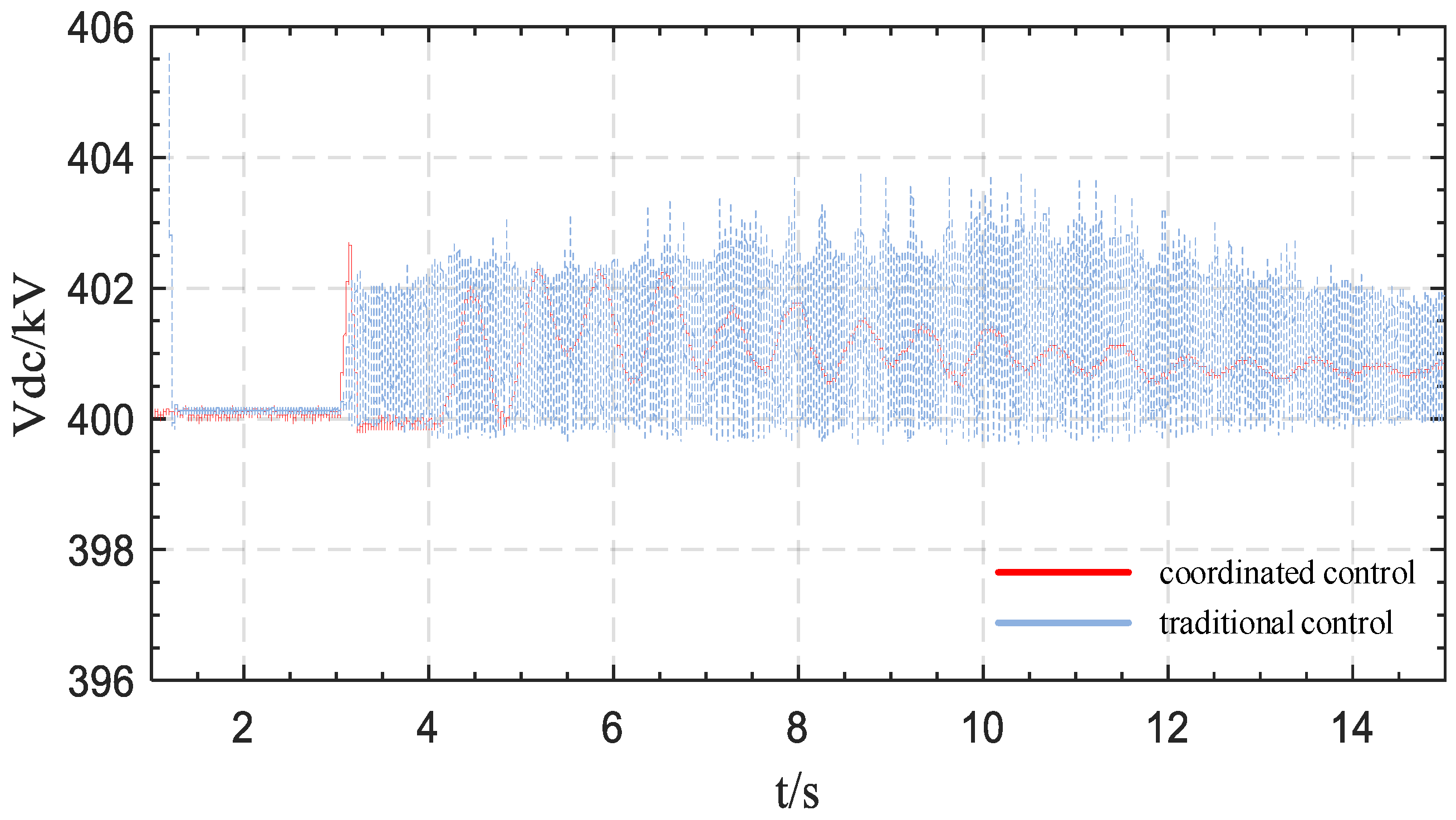
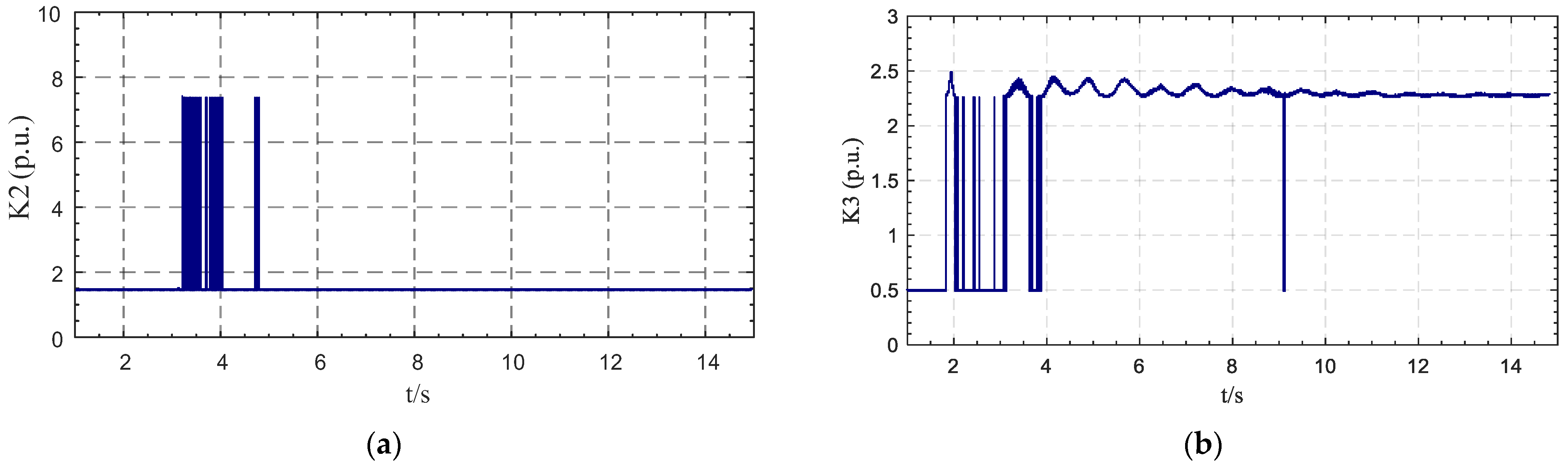
5. Experimental Results

5.1. Simulation Model

To validate the effectiveness of the proposed hybrid LCC-VSC DC transmission frequency control strategy, a simulation test system was constructed using the electromagnetic transient simulation software PSCAD/EMTDC v4.6.2, as illustrated in Figure 1.

The detailed parameters of the generator units are provided in reference [26]. The rated value of the DC voltage is 400 kV, with a permissible fluctuation range of ±5%. The LCC station adopts fixed active power control with a rated operating power of 350 MW, while theVSC2 and VSC3 stations use adaptive DC voltage droop control, with rated operating powers of 500 MW and 150 MW, respectively. The capacitance of the converter stations is set to C = 2000 μF. The distances from the LCC station and VSC3 station to the VSC2 station are both 200 km, connected by a DC cable with an impedance of 0.005 Ω/km. In Area 1, the wind farm has a rated capacity of 500 MVA, and generators G1, G2, G3, and G4 each have a rated capacity of 900 MVA, equipped with speed governor devices. However, only the generator in Area 1, G1, is equipped with AGC. The active power load is 900 MW in Area 1 and 1800 MW in Area 2.

5.2. Setup of Controller Parameters

Considering that the full-load power of VSC converter stations is 1.1 times the rated operating power. From (20) and (21), the initial droop coefficients of VSC2 and VSC3 are calculated to be K_H2 = 25, K_L2 = 2.5; K_H3 = 7.5, K_L3 = 1.5. The constant m in both cases is set to 0.007.

We run the simulation model in PSCAD/EMTDC. After the system reaches steady-state operation, we apply a 2% step disturbance to the set current controller of the LCC station at 2 s. We use the step disturbance to the set value as input and the speed difference between the selected generators G1 and G2 as output. We employ the VFF-RLS algorithm based system identification method to identify the open-loop system, obtaining the following:

$$G(s)={\displaystyle \frac{-0.0003015s^6-0.005026s^5-0.1082s^4-0.3252s^3-3.302s^2-0.3488s}{1.004s^6+3.4986s^5+87.83s^4+207.1s^3+1834s^2+2814.7s+214.8}}.$$

(23)

This study plots the root locus diagram of the system as derived from Equation (23), as shown in Figure 5. The root locus diagram of the system shown in Figure 5 indicates that all the poles of the system are located to the left of the imaginary axis, signifying stability. However, the dynamic characteristics of the open-loop system are determined by the pole $d_0=-0.137\pm 5.88\mathrm{i}$ nearest to the imaginary axis, which is isolated from other poles or zeros, resulting in weak damping with a damping ratio of 2.3%. To achieve better system dynamic characteristics, the desired damping ratio of the dominant closed-loop poles is ζ = 0.5, and the undamped natural oscillation frequency is ${\omega }_n=2\mathrm{rad}/\mathrm{s}$. The location of the dominant closed-loop poles is determined to be $s_d=-1\pm 1.7321\mathrm{i}$. Given that gain adjustment alone is insufficient to relocate the system’s dominant pole to the desired position, the introduction of a correction section is necessitated.

Substituting the dominant poles into Equation (10), it can be determined that T₁ = 3.4606, T₂ = 1.0125, and by substituting the already-determined parameters and calculating the amplitude condition, K_c = 280.2219. Thus, the final determined controller transfer function is as follows:

$$G_c(s)={\displaystyle \frac{750s+216.725}{s+0.9876}}.$$

(24)

Building upon the parameter tuning of the AFC controller, the optimization and solution for the PI controller parameters of AGC using the DQN algorithm yield the optimal values: K_P = 0.8, K_I = 0.4.

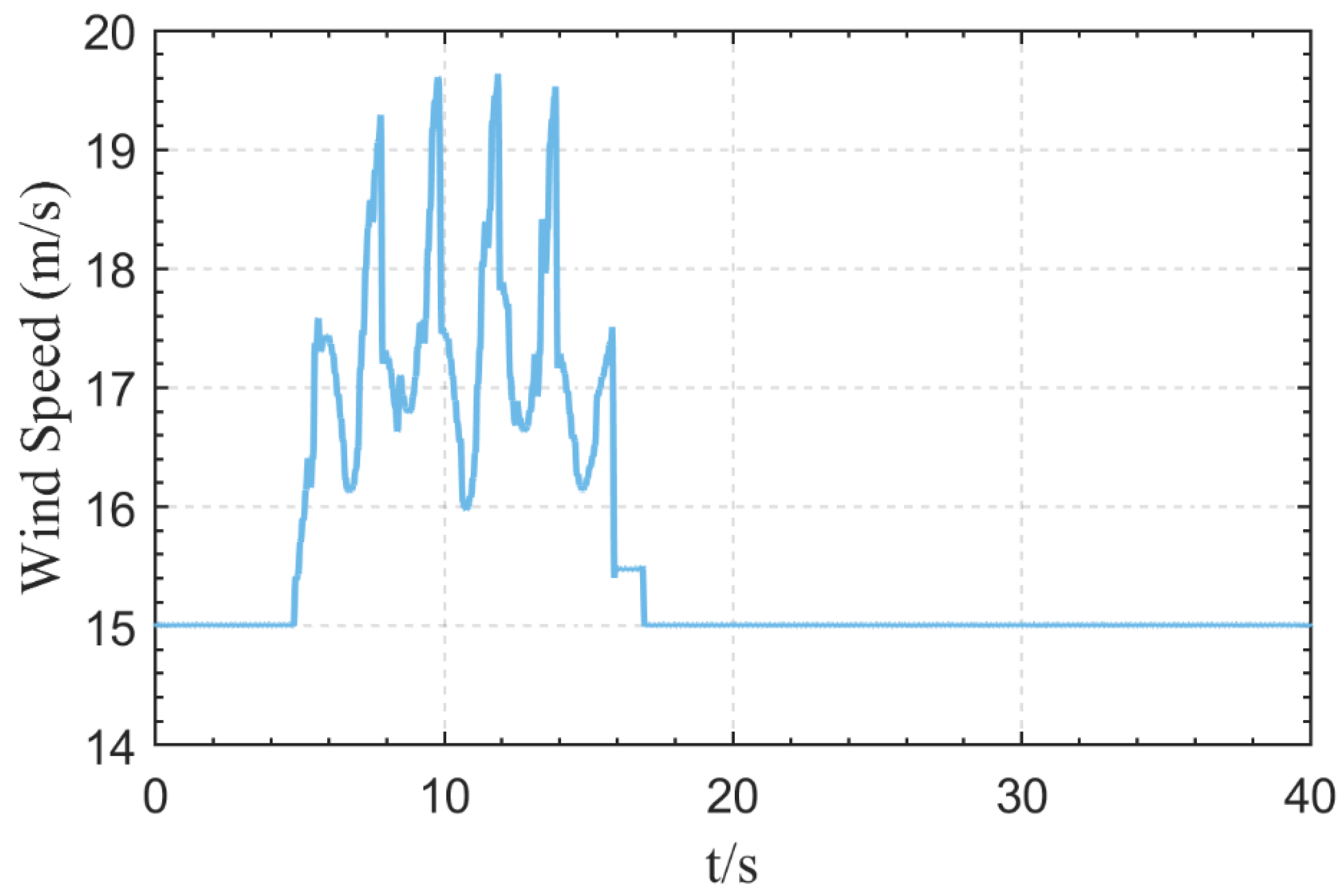
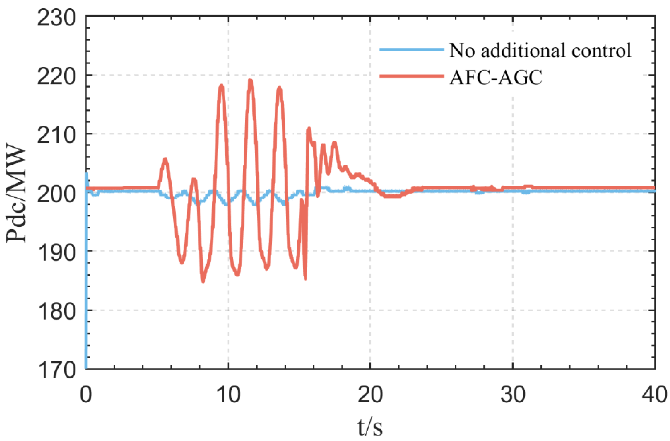
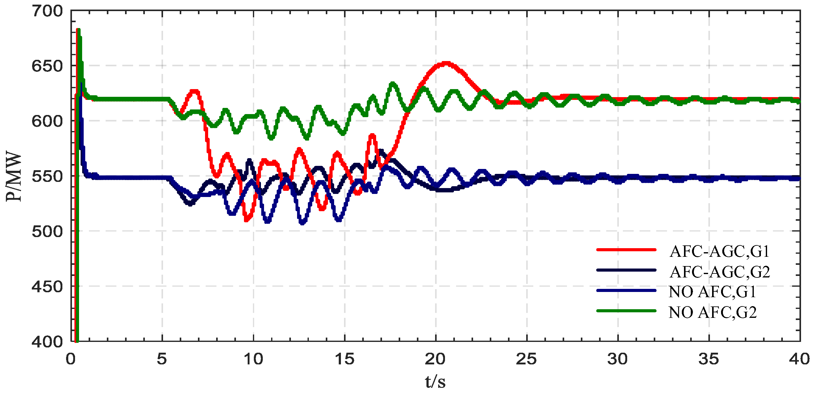
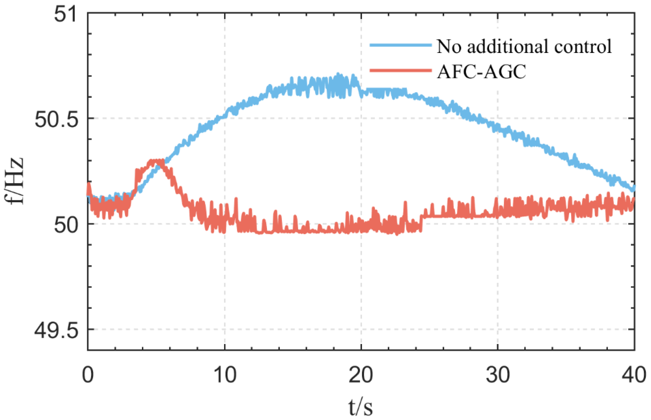
5.3. Case 1: Continuous Intense Fluctuations of Wind Speed

For Area 1, the wind speed fluctuations are systematically modeled, as illustrated in Figure 6. A comparison of simulation results is conducted between the proposed coordinated control strategy and the scenario without additional frequency control. The system frequency, DC link active power outputs from G1 and G2, and DC voltage are observed to assess the system’s frequency stability and power fluctuation regulation capability. The simulation results are presented in Figure 7, Figure 8 and Figure 9 for comparative analysis.

The comparison of system frequency changes shown in Figure 7 indicates that, with wind speed fluctuations, the frequency deviation exceeds +0.2 Hz approximately 2 s after initiation, continuously rising to 50.2 Hz. Within the 40 s simulation duration, the frequency exceeds the 50 ± 0.3 Hz range for a total of 20 s. At the end of the simulation, the frequency remains unstable, showing a large fluctuation range and a slow recovery process. Using the auxiliary frequency control strategy of AFC and AGC ensures that the frequency consistently remains within the 50 ± 0.2 Hz range throughout the simulation. Approximately 3 s following the cessation of wind speed fluctuations, the frequency promptly stabilizes at 50 Hz.

The observed variations in DC link active power and generator output are illustrated in Figure 8 and Figure 9. The results indicate that without auxiliary frequency control, the increment in wind power within Area 1 mainly relies on the isolated governor responses of generators G1 and G2, which adapt their outputs to assimilate this increase. However, this adjustment capability is notably constrained, and even after the cessation of wind speed fluctuations, the output from the generators continues to demonstrate minor yet persistent oscillations. When using the coordinated control strategy of AFC and AGC, the AGC unit G1 in Area 1 takes on the task of balancing most of the wind power increment. The auxiliary frequency controller promptly reacts to variations in wind power output that cause frequency fluctuations, issuing control commands that swiftly adjust the DC link transmission’s active power. After the stabilization of wind speed, both the DC link active power and the generator output rapidly regain stability.

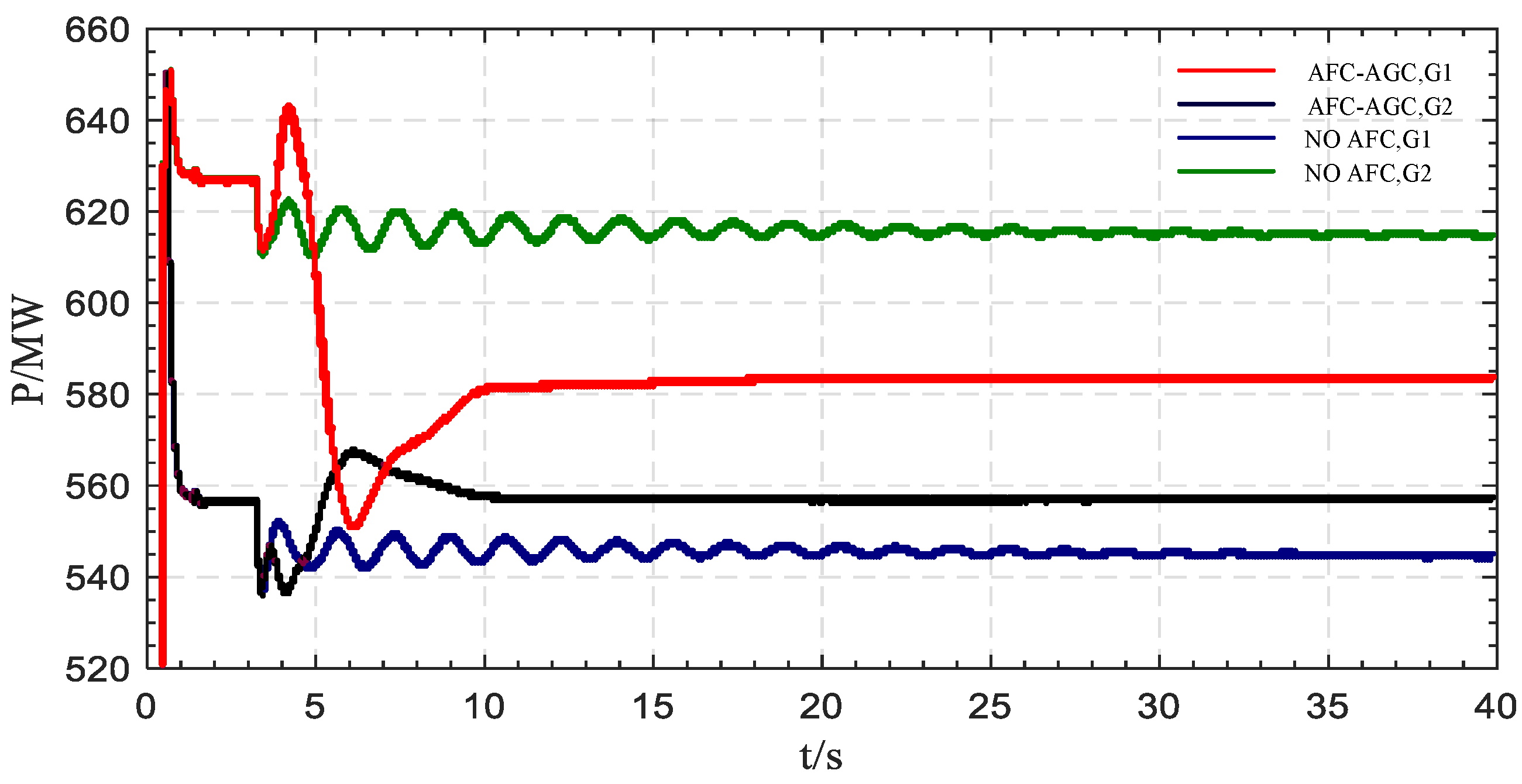
5.4. Case 2: Sudden Load Change

Introducing a load disturbance, in Area 1, at 3 s, there is a sudden loss of 40 MW in the active power load. The frequency, DC link active power, generator output, and voltage in Area 1 continue to be monitored. The simulation results are compared between no additional frequency control and those using AFC and AGC coordinated auxiliary frequency control strategy, as shown in Figure 10, Figure 11, Figure 12 and Figure 13.

According to the system frequency variation illustrated in Figure 10, following the abrupt reduction in load in Area 1, the surplus active power prompts an increase in the system frequency. In the absence of auxiliary frequency control, the frequency continues to rise, reaching a maximum deviation of up to 0.40 Hz, and then it slowly returns to a value close to the steady state around 38 s. In contrast, using the coordinated control strategy of AFC and AGC, the frequency peaks at approximately 50.3 Hz and, within about 5 s, swiftly reverts to the nominal value. Overall, the system frequency maintains a relatively stable condition.

As shown in Figure 11, generators G1 and G2 jointly address the active power disturbance, with their output changes mirroring each other, with both manifesting sustained oscillations after the disturbance. When implementing the coordinated control strategy, the AGC unit in G1 assumes the primary responsibility for the load disturbance, resulting in smoother changes in generator output. Due to the response of the AFC controller, the DC link engages in short-term adjustments, facilitating the system’s rapid return to steady-state operation within 10 s.

As illustrated in Figure 12 and Figure 13, it can be seen that the disturbance causes a change in DC voltage. The VSC2 station and VSC3 station, using the traditional control strategy, respond quickly, but the fixed droop coefficient fails to fulfill the adjustment demands, resulting in DC voltage oscillations. However, upon implementing the coordinated control strategy that includes adaptive DC voltage droop control and auxiliary frequency control, VSC2 and VSC3 stations effectively respond to DC voltage changes. They adaptively adjust the droop coefficient in real-time based on their own adjustment capacity and voltage fluctuations, thereby adjusting the active power of the converter station. The VSC2 station achieves the steady-state range following a brief adjustment period of approximately 1.6 s, thereafter requiring only minimal fine-tuning. The VSC3 station persistently responds to voltage fluctuations, continuously adjusting its power, and attains the steady-state range within approximately 8 s. This approach fully capitalizes on the VSC-MTDC’s capabilities for rapid and controllable active power adjustments, thereby enhancing the system’s frequency stability.

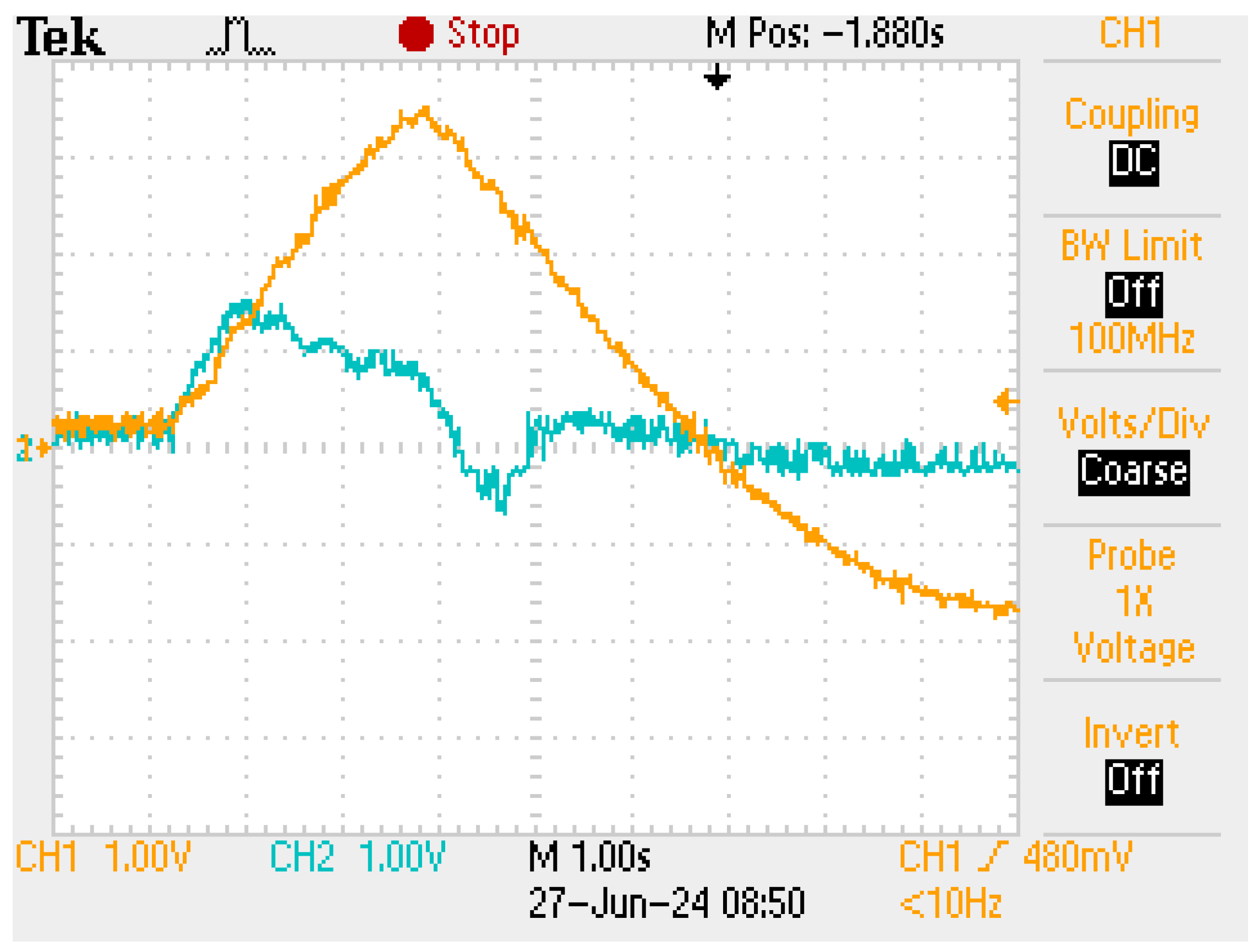
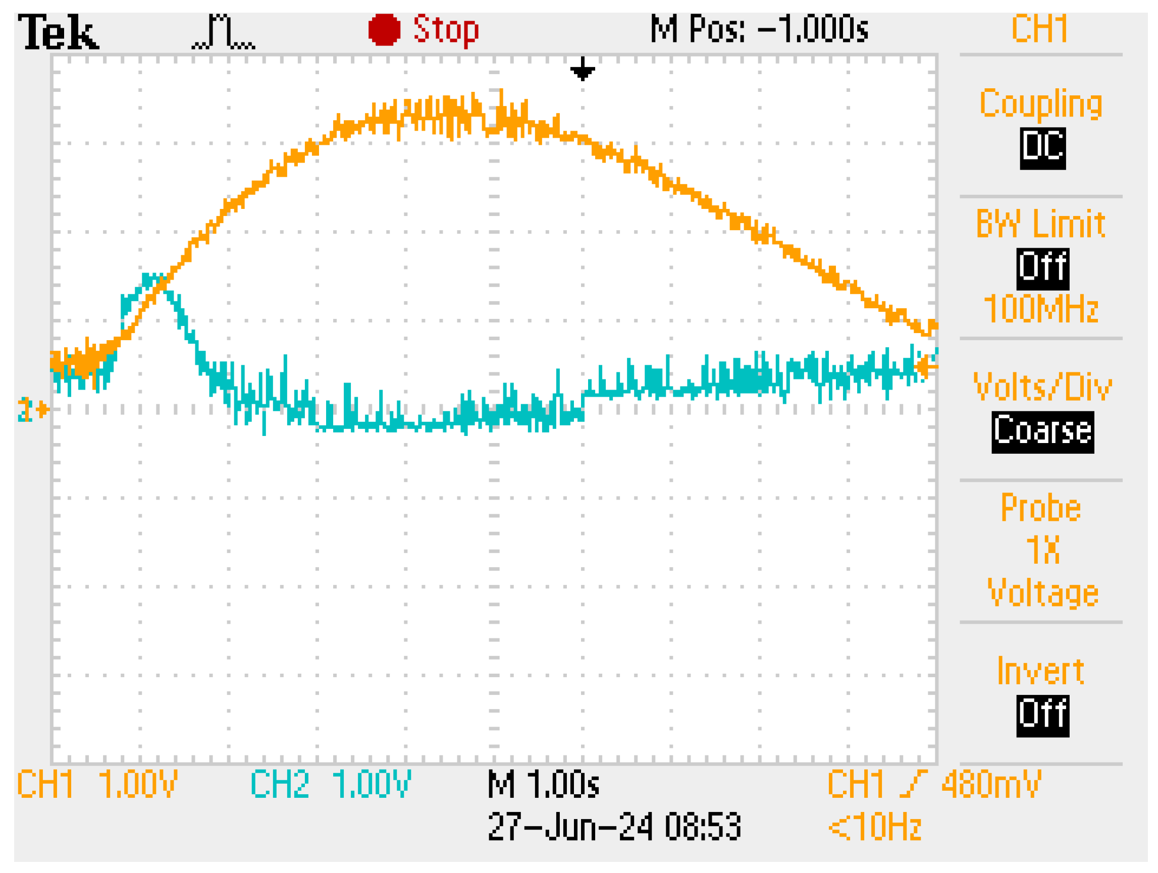
5.5. Experimental Verification

To further validate the proposed conclusions, a hardware platform based on controller hardware-in-the-loop (CHIL) was set up, as shown in Figure 14. This hardware platform consists of two parts: a control section based on TMS320F28335+FPGA, and a main circuit section simulated by Typhoon602+. The control section is responsible for sampling, computation, control, and waveform generation, while Typhoon602+ simulates the main circuit of a hybrid DC transmission system with wind power integration. The control board inputs the collected voltage and current data into the DSP. After executing the relevant calculations and controls, the DSP sends the waveform signals to the FPGA, which processes these signals and then sends them to Typhoon602+.

Figure 15 presents the frequency variation output waveforms under continuous and intense wind speed fluctuations. The yellow waveform represents the scenario without additional frequency control, while the green waveform depicts the scenario using the proposed control strategy. Figure 16 shows the frequency variation output waveforms after introducing load disturbances, with the yellow waveform again representing the scenario without additional control and the green waveform using the proposed strategy. By comparing these experimental results with the simulation results in Section 5.3 and Section 5.4, it can be observed that the experimental waveforms closely match the simulation waveforms. The introduction of auxiliary frequency control to participate in system frequency regulation enhances the frequency stability of the hybrid DC transmission system with wind power integration, further verifying the effectiveness of the proposed strategy.

6. Conclusions

In this paper, the LCC-VSC hybrid DC system, which integrates wind and hydro resources for transmission, is selected as the object of study. An auxiliary frequency control is introduced to participate in the frequency regulation of the system, and the following conclusions are obtained through simulation:

• The integration of large-scale wind power into the DC transmission system leads to continuous fluctuations in wind power output, significantly disturbing the system’s active power and adversely affecting the system’s frequency stability. Consequently, the primary frequency regulation of the system is no longer sufficient to meet the requirements. Therefore, utilizing the rapid controllability of DC transmission power provides a new perspective for improving the frequency regulation performance of the system.
• The control strategy, coordinated by both AFC and AGC, effectively mitigates the frequency fluctuations caused by the persistent and intense fluctuations of wind power output. Simultaneously, it demonstrates good frequency control performance under other disturbances, such as load mutations, thus enhancing the frequency stability of DC transmission systems integrated with wind power.

References

1. Xing, C.; Liu, M.; Peng, J.; Wang, Y.; Shang, C.; Zheng, Z.; Liao, J.; Gao, S. Frequency Stability Control Strategy for Voltage Source Converter-Based Multi-Terminal DC Transmission System. Energies 2024, 17, 1195. [Google Scholar] [CrossRef]
2. Fang, P.; Fu, W.; Wang, K.; Xiong, D.; Zhang, K. A compositive architecture coupling outlier correction, EWT, nonlinear Volterra multi-model fusion with multi-objective optimization for short-term wind speed forecasting. Appl. Energy 2022, 307, 118–191. [Google Scholar] [CrossRef]
3. Pali, B.S.; Vadhera, S. An Innovative Continuous Power Generation System Comprising of Wind Energy along with Pumped-Hydro Storage and Open Well. IEEE Trans. Sustain. Energy 2020, 11, 145–153. [Google Scholar] [CrossRef]
4. Wang, J.; Liao, Y.; Han, W.; Ding, J.; Yang, W. Modeling and active power control characteristics of pumped storage-wind hybrid power system in the context of peak carbon dioxide emission. Water Resour. Hydropower Eng. 2021, 52, 172–181. [Google Scholar]
5. Zhu, B.; Liu, Y.; Zhi, S.; Wang, K.; Liu, J. A Family of Bipolar High Step-Up Zeta–Buck–Boost Converter Based on “Coat Circuit”. IEEE Trans. Power Electron. 2023, 38, 3328–3339. [Google Scholar] [CrossRef]
6. Yang, N.; Dong, Z.; Wu, L.; Zhang, L.; Shen, X.; Chen, D.; Zhu, B.; Liu, Y. A Comprehensive Review of Security-constrained Unit Commitment. J. Mod. Power Syst. Clean Energy 2022, 10, 562–576. [Google Scholar] [CrossRef]
7. Xing, C.; Liu, M.; Peng, J.; Wang, Y.; Liao, J.; Zheng, Z.; Gao, S.; Guo, C. LCC-HVDC Frequency Robust Control Strategy Based on System Parameter Identification in Islanded Operation Mode. Electronics 2024, 13, 951. [Google Scholar] [CrossRef]
8. Wang, W.; Li, Y.; Cao, Y.; Häger, U.; Rehtanz, C. Adaptive Droop Control of VSC-MTDC System for Frequency Support and Power Sharing. IEEE Trans. Power Syst. 2018, 33, 1264–1274. [Google Scholar] [CrossRef]
9. Xisheng, T.; Fufeng, M.; Zhiping, Q.I.; Huimin, H.E.; Tao, W.U.; Shanying, L.I. Survey on Frequency Control of Wind Power. Proc. CSEE 2014, 34, 4304–4314. [Google Scholar]
10. Curtice, D.H.; Reddoch, T.W. An Assessment of Load Frequency Control Impacts Caused by Small Wind Turbines. IEEE Trans. Power Appar. Syst. 1983, PAS-102, 162–170. [Google Scholar]
11. Machowski, J.; Bialek, J.W.; Bumby, J.R. Power System Dynamics; Wiley: Hoboken, NJ, USA, 2013. [Google Scholar]
12. Meza, J.L.; Santibanez, V.; Soto, R.; Llama, M.A. Fuzzy Self-Tuning PID Semiglobal Regulator for Robot Manipulators. IEEE Trans. Ind. Electron. 2012, 59, 2709–2717. [Google Scholar] [CrossRef]
13. Hong, Z.; Xu, W.; Lv, C.; Ouyang, Q.; Wang, Z. Deep reinforcement learning-PI control strategy of air servo system based on genetic algorithm optimization. J. Mech. Electr. Eng. 2023, 40, 1071–1078. [Google Scholar]
14. Shi, J.; Li, S.; Zhao, N.; Xu, M. Constrained Adaptive PI Control of Inverter based on Neural Network. Acta Energiae Solaris Sinca 2023, 44, 19–27. [Google Scholar]
15. Li, B.; Wang, J.; Liang, S.; Wei, C. AGC real-time control strategy based on LSTM recurrent neural network. Electr. Power Autom. Equip. 2022, 42, 128–134. [Google Scholar]
16. Liu, H.; Xu, F.; Fan, P.; Liu, L.; Wen, H.; Qiu, Y.; Ke, S.; Li, Y.; Yang, J. Load Frequency Control Strategy of Island Microgrid with Flexible Resources Based on DQN. In Proceedings of the 2021 IEEE Sustainable Power and Energy Conference (iSPEC), Nanjing, China, 23–25 December 2021; pp. 632–637. [Google Scholar]
17. Jiang, B.; Wang, Q.; Wu, S.; Wang, Y.; Lu, G. Advancements and Future Directions in the Application of Machine Learning to AC Optimal Power Flow: A Critical Review. Energies 2024, 17, 1381. [Google Scholar] [CrossRef]
18. Zhou, X.; Wang, Y.; Shi, Y.; Jiang, Q. Deep Reinforcement Learning-Based Optimal PMU Placement Considering the Degree of Power System Observability. IEEE Trans. Ind. Inform. 2024, 20, 8949–8960. [Google Scholar] [CrossRef]
19. He, C.; Wang, H.; Wei, Z.; Wang, C. Distributed Coordinated Real-Time Control of Wind Farm and AGC Units. Proc. CSEE 2015, 35, 302–309. [Google Scholar]
20. Xu, Y.; Mili, L.; Sandu, A.; von Spakovsky, M.R.; Zhao, J. Propagating Uncertainty in Power System Dynamic Simulations Using Polynomial Chaos. IEEE Trans. Power Syst. 2019, 34, 338–348. [Google Scholar] [CrossRef]
21. Xu, Y.; Wang, Q.; Mili, L.; Zheng, Z.; Gu, W.; Lu, S.; Wu, Z. A Data-Driven Koopman Approach for Power System Nonlinear Dynamic Observability Analysis. IEEE Trans. Power Syst. 2023, 39, 4090–4104. [Google Scholar] [CrossRef]
22. Yan, M.; Cai, H.; Xie, Z.; Zhang, Z.; Xu, Z. Distributed DC voltage control strategy for VSC-MTDC systems. Electr. Power Autom. Equip. 2020, 40, 134–140. [Google Scholar]
23. Hu, J.; Zhao, C. In auxiliary frequency control of HVDC systems for wind power integration. In Proceedings of the 2010 5th International Conference on Critical Infrastructure (CRIS), Beijing, China, 20–22 September 2010; pp. 1–5. [Google Scholar]
24. Rong, M.; Wu, H.; Wu, T.; Hou, X.; Zhang, J.; Yu, B. Improved V/F control strategy for enhancing stability of Direct-drive wind power with VSC-HVDC system. Power Syst. Technol. 2021, 45, 1698–1706. [Google Scholar]
25. Aljabrine, A.A.; Smadi, A.A.; Chakhchoukh, Y.; Johnson, B.K.; Lei, H. Resiliency Improvement of an AC/DC Power Grid with Embedded LCC-HVDC Using Robust Power System State Estimation. Energies 2021, 14, 7847. [Google Scholar] [CrossRef]
26. Kundur, P. Power System Stability and Control; CRC press: Boca Raton, FL, USA, 1994. [Google Scholar]
Figure 1. Hybrid LCC-VSC transmission system.
Applsci 14 06817 g001
Figure 2. System structure of the AFC controller.
Applsci 14 06817 g002
Figure 3. Diagram of the control system.
Applsci 14 06817 g003
Figure 4. Diagram of AGC structure.
Applsci 14 06817 g004
Figure 5. Root Locus diagram of the system.
Applsci 14 06817 g005
Figure 6. Wind speed variations.
Applsci 14 06817 g006
Figure 7. Comparison of system frequency variations.
Applsci 14 06817 g007
Figure 8. Comparison of DC link active power variations.
Applsci 14 06817 g008
Figure 9. Comparison of G1 and G2 output variations.
Applsci 14 06817 g009
Figure 10. Comparison of system frequency variations.
Applsci 14 06817 g010
Figure 11. Comparison of changes in generator output.
Applsci 14 06817 g011
Figure 12. Variation of DC voltage with different control strategies.
Applsci 14 06817 g012
Figure 13. Variation of droop coefficients with coordinated control strategy: (a) VSC2-droop coefficient; (b) VSC3-droop coefficient.
Applsci 14 06817 g013
Figure 14. Hardware platform of CHIL experiment.
Applsci 14 06817 g014
Figure 15. Case 1 experimental results: comparison of system frequency changes.
Applsci 14 06817 g015
Figure 16. Case 2 experimental results: comparison of system frequency changes.
Applsci 14 06817 g016