A Prediction Method for the Average Winding Temperature of a Transformer Based on the Fully Connected Neural Network

Abstract

The average winding temperature of a transformer (AWTT), serving as a key indicator for assessing the running state of the transformer, is of utmost importance in determining a transformer’s electrical properties and the insulation longevity of the transformer. An accurate prediction of AWTT is essential for ensuring the safe operation of the transformer. A novel method for predicting AWTT is introduced based on the analysis of field monitoring data. Firstly, the thermal characteristics and operational mechanisms of oil-immersed transformers are examined. Secondly, a factor analysis model is developed to streamline the network structure, accounting for the strong correlations among ambient temperature, load current, and top oil temperature. Thirdly, the independent temperature factor and load factor are extracted as pivotal features, and then input into the fully connected neural network to predict AWTT. Through a case study involving a 110 kV/10 kV oil-immersed transformer, the results show that the proposed method reduces redundant correlation information compared to traditional methods and improves the prediction accuracy of AWTT, establishing a foundation for further transformer state assessments.

1. Introduction

Power transformers, as the key component in transmission and distribution systems, play a significant role in power systems. The average winding temperature (AWTT) and the winding hot-spot temperature (WHSTT) serve as critical parameters for assessing the transformer’s state [1,2,3,4]. Elevated AWTT can accelerate the degradation of insulation materials, escalate transformer losses, and compromise insulation strength, increasing the risk of equipment malfunctions and accidents. Therefore, the accurate prediction of AWTT is essential for enabling operation and maintenance personnel to promptly identify potential issues and implement protective measures to ensure safe operation of the transformer [5,6,7,8].

Currently, the methods for predicting the AWTT and WHSTT are mainly following: empirical thermal model method, thermal circuit model method, numerical simulation method, and artificial intelligence method. The most used method for calculating AWTT is the empirical thermal model, as in [9,10]. This method utilizes one or two differential equations to describe the increase in the AWTT in relation to the top oil temperature. Another method is the thermal circuit equivalent model method. In [11], nonlinear thermal resistance is introduced into the thermal path model to solve the problem of uneven heat transfer inside the transformer, and the temperature rise of the transformer winding is predicted by using this model, and a good calculation result is obtained, providing a new example for studying the hot-spot temperature rise of winding by using the thermal path model. In [12], by discussing the influence of oil viscosity and resistance on thermal resistance, the thermal resistance is redefined, which makes the calculation of thermal resistance more practical and improves the lumped thermal path model. However, both the empirical thermal model and the thermal circuit equivalent model bring challenges because parameters such as winding index, oil index, and thermal constant are typically approximated based on the transformer capacity and cooling methods. Therefore, the accuracy of these models in calculating the AWTT is limited in practical applications. Considering the winding structure and loss distribution comprehensively, numerical simulation analysis enables precise calculation of the AWTT. In [13], the finite element method analyzed the magnetic field and transformer loss, and the finite volume method calculated the temperature distribution, considering material property changes. In [14,15], scholars studied the influence of parameters such as oil passage size and baffle structure on winding temperature to provide guidance for transformer heat dissipation design. Artificial intelligence algorithms can predict the AWTT accurately by analyzing the operational data, environmental factors, and winding characteristics of the transformers. In [16], a model using the kernel extreme learning machine was created to predict the top layer oil temperature of transformers, accounting for uncertainty and matching measured values. In [17], particle swarm optimization improved this model by considering environmental factors, enhancing prediction accuracy.

However, due to the complex and variable operating conditions of the transformers, the current methods for predicting AWTT have some problems.

Table 1. The inadequacies of existing research methods.

Method	Inadequacy
Empirical thermal model method	Lack of accuracy, dependent on specific conditions
Thermal circuit model method	The solving model is relatively complex and computationally heavy
Numerical simulation method	High computing resource requirements and complex model building

shows the inadequacies of existing research methods. The mutual influence of factors such as heat conduction, cooling, and losses within the windings makes it difficult for traditional models to provide accurate simulations. Generally, these models rely on oversimplified assumptions and empirical equations, which do not simulate the complex heat conduction process within transformers effectively. Consequently, the accuracy and reliability of current prediction methods for AWTT are limited. Therefore, it is necessary for further research to address these challenges.

The thermal properties and operational mechanisms of oil-immersed transformers are analyzed to address the issues in this paper. A predictive model for AWTT is introduced, which is based on the fully connected neural network. Firstly, the thermal properties of oil-immersed transformers are analyzed, and there is coupling among ambient temperature, load current, and top oil temperature. Secondly, the above parameters are decoupled based on the factor analysis, implementing the effect of reducing the input dimension. Thirdly, the fully connected neural network is used to predict the AWTT. Finally, the analysis and verification are conducted on real transformer data, and the results show that the proposed method improves the prediction accuracy of the AWTT with reduced dimensions of data processing compared to traditional methods. The method in this paper is meaningful for attaining AWTT accurately and can offer support for further transformer state assessments.

2. Analysis of the Thermal Properties of Oil-Immersed Transformers

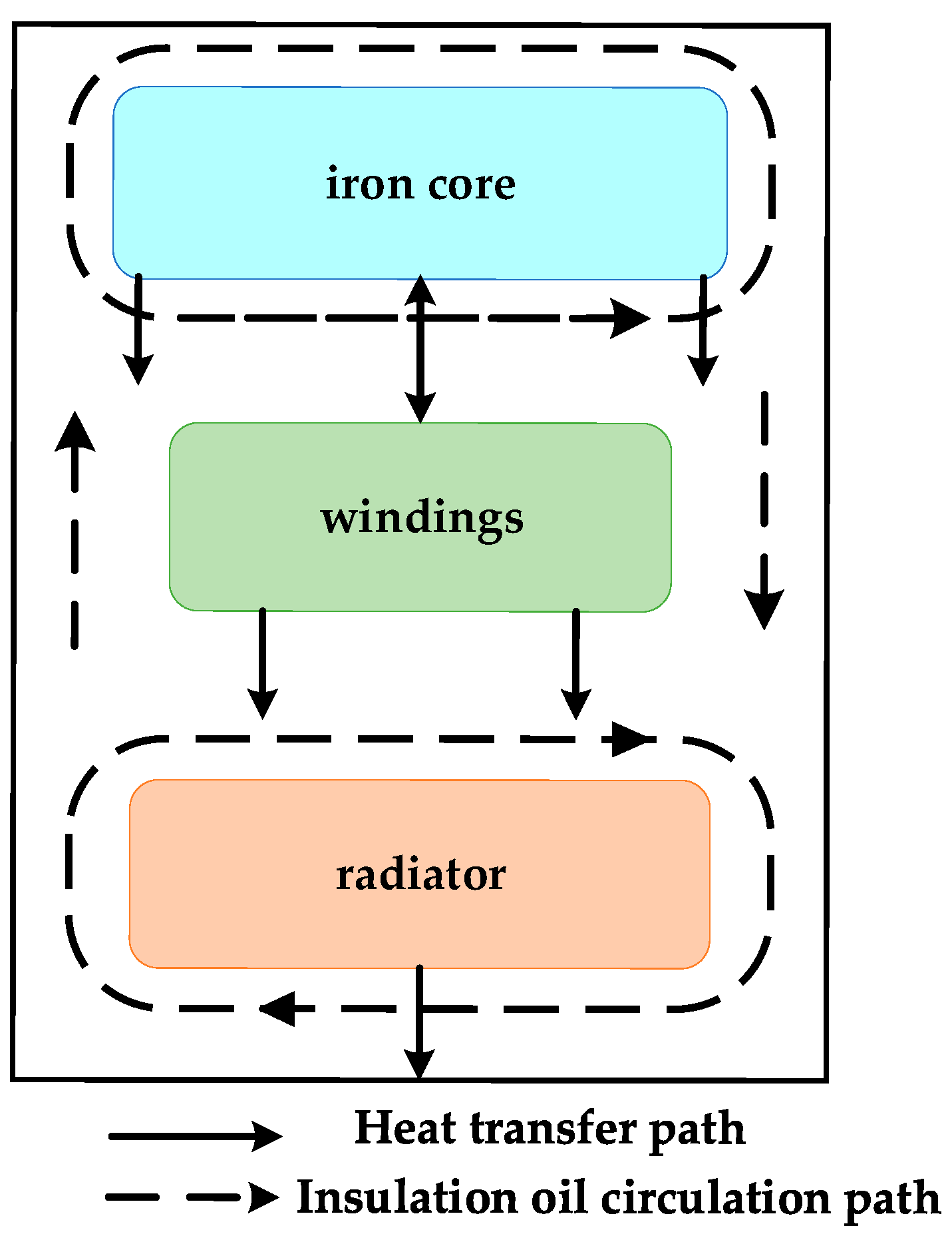
2.1. Internal Heat Generation Mode of Oil-Immersed Transformer

During the operation of transformers, internal heat is generated due to the copper losses in the windings, iron losses in the core, and stray losses in the transformer components under leakage magnetic flux. The copper loss can be expressed as follows:

$$P=3I_{1N_{\varphi }}^2{R}_{1.75°\mathsf{C}}+3I_{2N_{\varphi }}^2{R}_{2.75°\mathsf{C}}$$

(1)

where $P$ is the copper loss, and $I_{1N_{\varphi }}$ and $I_{2N_{\varphi }}$ are the phase current of the primary and secondary transformer windings, respectively. $R_{1.75°\mathsf{C}}$ and $R_{2.75°\mathsf{C}}$ are the total resistance of the primary and secondary transformer windings converted to 75 °C, respectively.

The iron loss is expressed as follows:

$$P_0=K_{0}G{P}_C$$

(2)

$$P_C=P_{1/50}{(F/50)}^{\beta }{B}_m^2$$

(3)

where $P_0$ is the iron loss, $K_0$ is the loss technological coefficient and takes the value 0.9, G is the core weight, $P_C$ is the loss per unit weight, $P_{1/50}$ is the iron loss coefficient, $\beta$ is the frequency index, and $B_m$ is the maximum magnetic flux density of the core.

Compared with the former two types of losses, the stray loss in the transformer is generated by the leakage magnetic field in the conductive material, usually with a smaller value [18,19,20].

2.2. Internal Heat Transfer Process of Oil-Immersed Transformer

The heat transfer in oil immersed transformers is mainly influenced by conduction and convection diffusion, while radiation has a relatively small heating effect. In particular, between conduction and convection, the former is the key to heat transfer. During operation, some losses in the transformer result in heat within the core and windings, and part of this heat is transferred to the insulating oil through conduction. The volume and temperature of the insulating oil are closely linked, as heat absorption causes the oil to expand. Thus, the oil density is reduced, and the oil flow characteristics are changed. This heat is then dissipated to the outside in a convective manner, as illustrated in Figure 1.

3. Prediction of AWTT

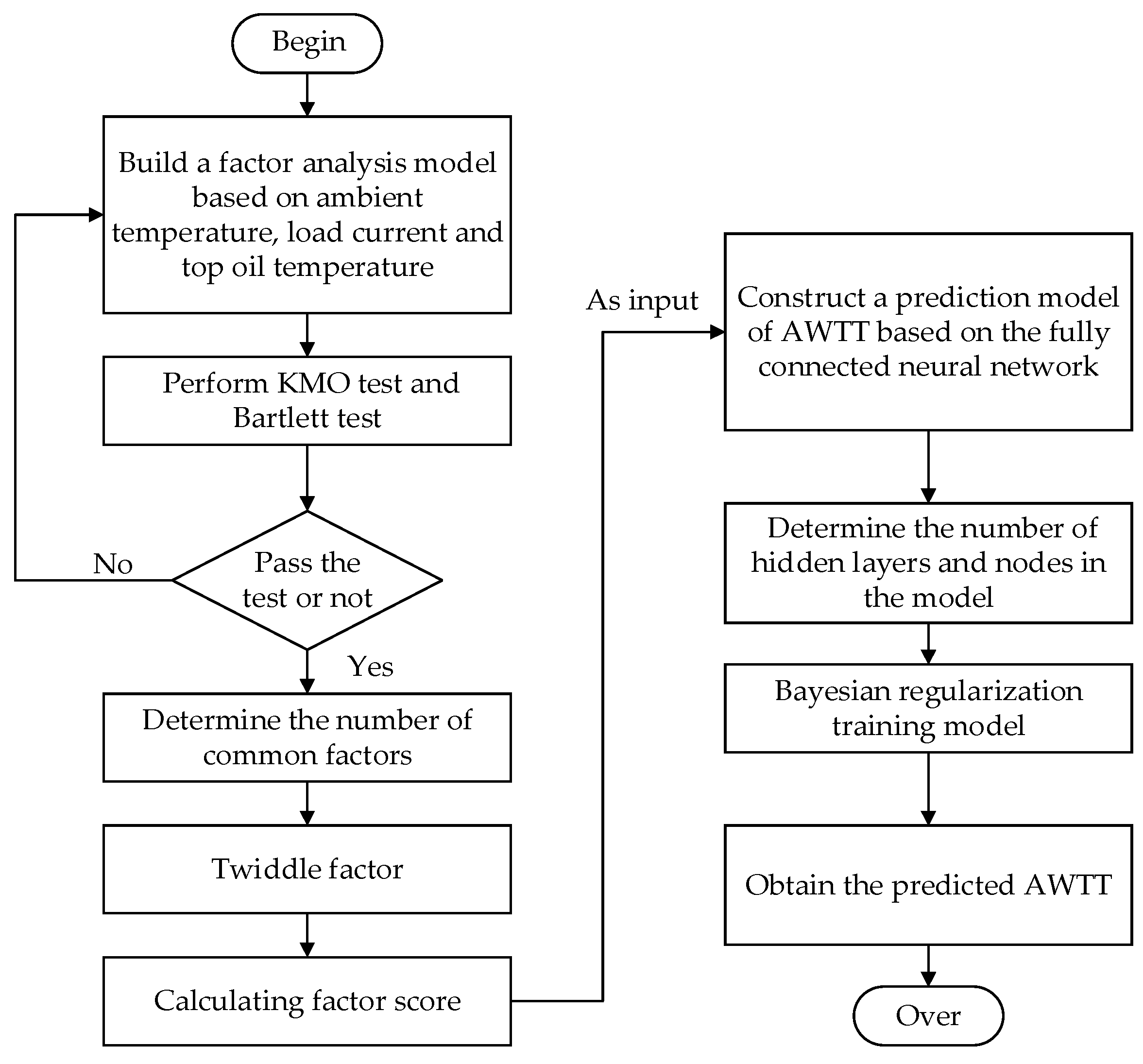
3.1. Correlation Analysis of Original Variables

The load borne by the transformer is real-time fluctuations during the operation. The heat transfer process includes the heat generated by load loss at the corresponding moment. This process is continuous and uninterrupted, so the AWTT is dynamic, influenced by ambient temperature, oil temperature, load [18], wind velocity [21], harmonics [22], insulation paper [23], and solar radiation [24]. In the on-site situation, the placement of sensors is relatively strict, and some parameters are inconvenient to measure. In addition, if the cooling method of the transformer is ONAN, it is impossible to assign initial values to the oil flow velocity and fit the oil flow direction through mathematical formulas. Therefore, ambient temperature, load current, and top oil temperature, affecting the temperature elevation characteristics of transformers, are selected as the fundamental parameters to predict AWTT.

Figure 2 shows the trend of data points in the scatter plot clearly among ambient temperature, load current, and top oil temperature. The purple are data points. The orange shows the relationship between top oil temperature and load current. The blue shows the relationship between top oil temperature and ambient temperature. The green shows the relationship between ambient temperature and load current. Preliminary assessments are conducted on the correlation between these three key parameters. With the increase in one characteristic parameter, another characteristic parameter also tends to rise, indicating a rough positive linear correlation between any pair of the parameters within the three.

In order to obtain more accurate and reliable results for quantitative analysis, the Pearson correlation coefficient is adopted to further analyze the numerical correlation among ambient temperature, load current, and top oil temperature. The Pearson correlation coefficient can assess the correlation between two variables, and the calculated value is within the range of −1 to 1 and can be expressed as follows:

$${\rho }_{X,Y}={\displaystyle \frac{s(X,Y)}{{\sigma }_X{\sigma }_Y}}={\displaystyle \frac{{\displaystyle \sum _{i=1}^n(X_i-\overline{X})(Y_i-\overline{Y})}}{\sqrt{{\displaystyle \sum _{i=1}^n{(X_i-\overline{X})}^2{\displaystyle \sum _{i=1}^n{(Y_i-\overline{Y})}^2}}}}}$$

(4)

where $s$ is covariance; ${\sigma }_X$ and ${\sigma }_Y$ are the standard deviations of variables X and Y; $\overline{X}$ and $\overline{Y}$ are the average values of X and Y; n is the number of samples; and $X_i$ and $Y_i$ are the variables, respectively.

In accordance with the correlation coefficient in

Table 2. Correlation coefficient of ambient temperature, load current, and top oil temperature.

	Ambient Temperature	Load Current	Top Oil Temperature
Ambient temperature	1	0.657	0.793
Load current	0.657	1	0.724
Top oil temperature	0.793	0.724	1

, the correlation coefficients among the ambient temperature, load current, and top oil temperature are all above 0.6. Among them, the strongest correlation is found between the top oil temperature and the ambient temperature. The transformer dissipates internally generated heat to the external environment through the heat dissipation system. Radiation and convection are driven by temperature differences. Both are impacted by ambient temperature, changing the top oil temperature. Furthermore, the transformer is an intercoupling thermal system. The thermal coupling effect also results in a strong positive correlation between the load current and the top oil temperature. When the load current passes through the winding, resistance and eddy current loss are generated. The heat converted by the loss is transmitted to the cooling medium transformer oil through the heat transfer mode, causing an increase in the oil temperature. In addition, the increase in load current will lead to the accumulation of heat inside the transformer. The heat is dissipated to the external environment, affecting ambient temperature distribution.

3.2. Factor Analysis Feature Dimension Reduction

A notable correlation among ambient temperature, load current, and top oil temperature is observed as mentioned above. If these three highly correlated parameter data are directly used to predict the AWTT, there will be an abundance of superfluous information, potentially leading to the problem of over-fitting and the complexity of prediction models. The factor analysis algorithm can effectively decouple and improve the efficiency of the network model. Based on retaining the main original data information, the correlation between the data is removed, and the dimensionality of the data is reduced.

Ambient temperature x₁, load current x₂, and top oil temperature x₃ are selected as three evaluation indexes in this paper. When there are n samples, a data matrix of $n\times 3$ can be expressed as

$$x=\left(\begin{array}{ccc}{x}_{11}& x_{12}& x_{13}\\ x_{21}& x_{22}& x_{23}\\ ⋮& ⋮& ⋮\\ x_{n1}& x_{n2}& x_{n3}\end{array}\right)=\left(x_1,x_2,x_3\right)$$

(5)

The ambient temperature, load current, and top oil temperature are represented as a linear combination of common factors and special factors, so as to establish the factor analysis model. Then, the Kaiser–Meyer–Olkin (KMO) test and Bartlett test are performed on the data. Following the confirmation of significant correlations, the quantity of common factors is determined. Factor rotation is executed to minimize bias and enhance the explication of the practical implications. Finally, the Anderson–Rubin method is used to compute the factor scores. According to the component score coefficient matrix, the coefficients of the factor score function are obtained, resulting in the acquisition of all factor scores. That is, the common factor is represented as a linear combination of the original variables.

$$\{\begin{array}{l}{f}_1=b_{11}{x}_1+b_{12}{x}_2+b_{13}{x}_3\\ f_2=b_{21}{x}_1+b_{22}{x}_2+b_{23}{x}_3\\ \cdots \\ f_m=b_{m1}{x}_1+b_{m2}{x}_2+b_{m3}{x}_3\end{array}$$

(6)

where $f_1,f_2,\cdots ,f_m(m<3)$ is the common factor, and $b_{ij}$ is the coefficient of the ith factor corresponding to the jth variable.

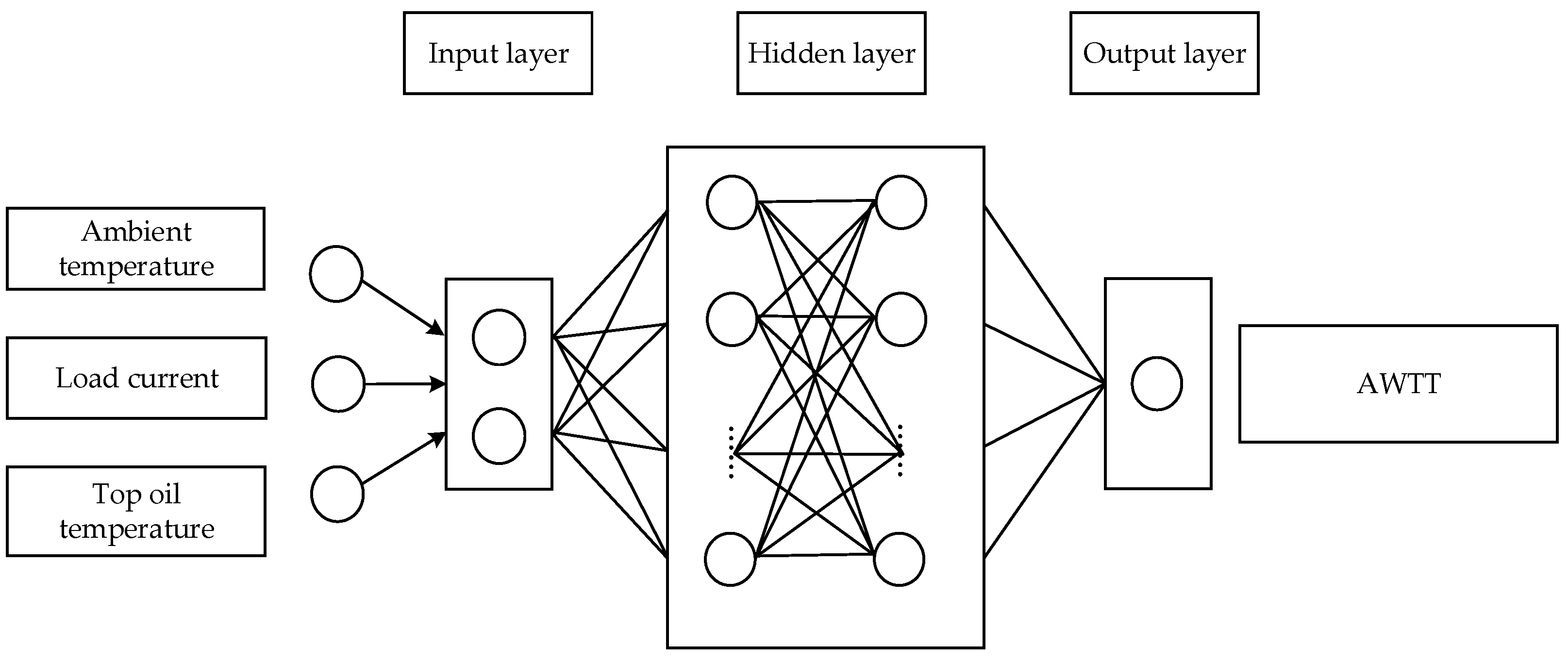
3.3. Constructing Fully Connected Neural Networks

With its robust expression capabilities, favorable capacity for nonlinear data fitting, and strong generalization ability, the fully connected neural network can accurately learn and represent the complex nonlinear mapping relationships between input features and output parameters. It is a commonly used method to achieve accurate prediction of low dimensional nonlinear data. Therefore, a fully connected neural network is used to predict the AWTT. The factor score derived from the above factor analysis is the input of the network model, and the AWTT is the output. This method constructs a prediction model for the AWTT using the fully connected neural network, as shown in Figure 3.

The neural network mentioned above is trained with the Bayesian regularization optimization algorithm. This algorithm utilizes maximum a posteriori to infer estimated model parameters, automatically determining appropriate regularization parameters. This method helps prevent overfitting and enhances the model generalization ability.

3.4. Prediction Method for AWTT

As shown in Figure 4, the method for predicting AWTT involves the factor analysis and the fully connected neural network. Firstly, the factor model is established among ambient temperature, load current, and top oil temperature. Then, the above parameters are decoupled based on the factor analysis. Next, taking the factor score as the input and the AWTT as the output, the AWTT prediction model based on the fully connected neural network is constructed, and the hidden layers and the number of nodes are adjusted. Finally, the model trained with the Bayesian regularization optimization algorithm is applied to predict the AWTT.

4. Case Verification

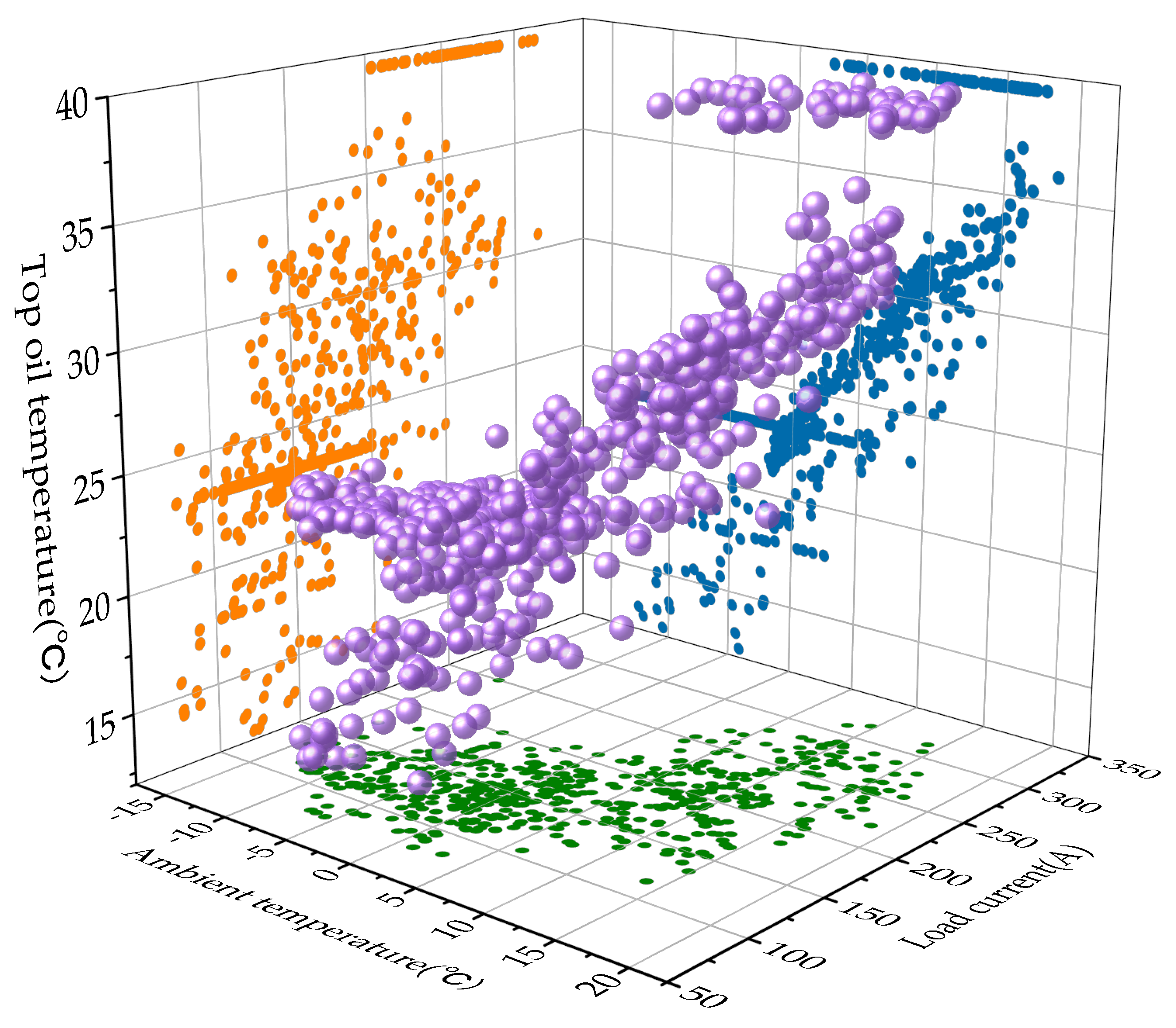
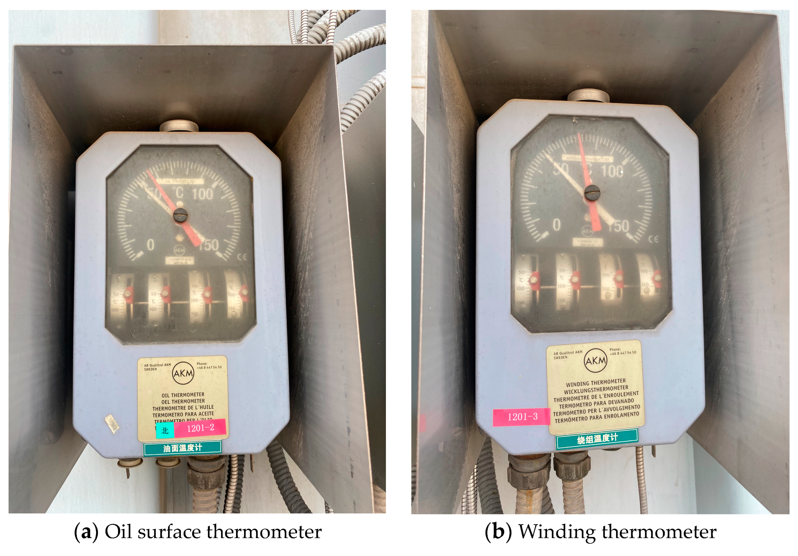
4.1. Field Test

The field monitoring data of a 110 kV oil-immersed transformer in a substation are selected as the experimental data set in this paper. The model of the transformer is SSZ11-50000/110, and the basic parameters are shown in

Table 3. SSZ11-50000/110 basic parameters.

Parametric Index	Value	Parametric Index	Value
Rating capacity	50,000/50,000/50,000 kVA	Connection group	YNyn0d11
Rating voltage	110 ± 8 × 1.25%/36.75/10.5 kV	Impedance voltage	10.3/18.73/6.81%
Rating current	262.4/785.5/2749.3 A	No load current	0.09%
Frequency	50 Hz	Cooling method	ONAN
Number of phases	3	Oil surface temperature rise	55 K
Upper oil tank weight	6700 kg	Oil weight	20,300 kg

. These parameters are from the nameplate of the transformer. Figure 5 shows the transformer physical diagram.

The data set includes the ambient temperature, load current, top oil temperature, and AWTT of the selected transformer. There are 560 groups of data samples. The on-site temperature data in the substation are from the dedicated detection device for transformer oil temperature and the winding thermometer, as shown in Figure 6. The oil temperature sensor is installed inside the oil tank near the top cover to measure the top oil temperature. The AWTT is measured with the winding thermometer. The temperature measured with the winding thermometer is actually the temperature of the top oil layer and the temperature rise of the coil to the oil. It is based on the oil temperature gauge and is equipped with the current matching device and the electric heating element. The oil temperature probe is 20–30 cm away from the top of the transformer. The current matching device is a type of current conversion device. The current output from the current transformer is converted into the heating current to the electric heating element, thereby simulating the AWTT. When a certain phase does not bear power, the temperature rise of the coil to the oil is zero, and the reading on the winding thermometer is the temperature of the transformer oil. When the phase bears power and operates, the current of the current transformer is converted into a heating current through the current matching device. The electric heating element is heated and corresponding additional displacement is generated. The temperature indicated with the winding thermometer is the sum of the top oil temperature and the temperature rise of the coil to the oil.

The working condition data of the transformer come from the terminal management system of the substation operation and maintenance team. Figure 7 shows the load changes in the transformer within a week. From the load data, the transformer operates at low load, and the maximum load carried by the transformer fluctuates in numerical values. However, the trend of load changes is basically the same. The peak load occurs from noon to evening, corresponding to the peak electricity consumption period in the vicinity of the transformer. The minimum load value occurs in the early morning, which is a low valley for application electricity.

4.2. Data Preprocessing

The factor analysis algorithm is used to preprocess the ambient temperature, load current, and top oil temperature in the above data set. After the establishment of the factor model, the KMO test and the Bartlett test are first performed. According to KMO = 0.723, the p value of the Bartlett test is less than 0.001, so this group of data is suitable for factor analysis.

Table 4. Total variance explanation table.

Total Variance Interpretation
Factor	Initial Eigenvalue			Extract the Sum of Squared Loads			Rotating Load Sum of Squares
	Total	Variance %	Accumulate %	Total	Variance %	Accumulate %	Total	Variance %	Accumulate %
1	2.451	81.688	81.688	2.451	81.688	81.688	1.610	53.652	53.652
2	0.353	11.775	93.463	0.353	11.775	93.463	1.194	39.811	93.463
3	0.196	6.537	100.000	/	/	/	/	/	/

shows the variance and cumulative sum explained by each common factor. From the initial eigenvalues, the variance percentage of the first common factor is 81.688. It represents that 81.688% of the information of the original variable can be explained by the first common factor. The percentage of variance of the second common factor is 11.775, so the second common factor can explain 11.775% of the information in the original variable. The cumulative variance of the first two common factor explanations is 93.463%. These two common factors already contain most of the variability of the original data and effectively summarize the main features of the original data set. However, the subsequent common factors have little contribution to the interpretation of the original variables, so the first two common factors are extracted for analysis and prediction tasks. The square sum of extracted loads is the variance contribution information of the two common factors extracted without rotation. The values are the same as the first two rows of initial eigenvalues. The square sum of rotational loads is the variance contribution information of the new common factor obtained after rotation, which helps distinguish and explain different factors. Compared with the unrotated contribution information, the variance contribution rate of each common factor changes, but the final cumulative variance contribution rate remains unchanged at 93.463%.

(1)

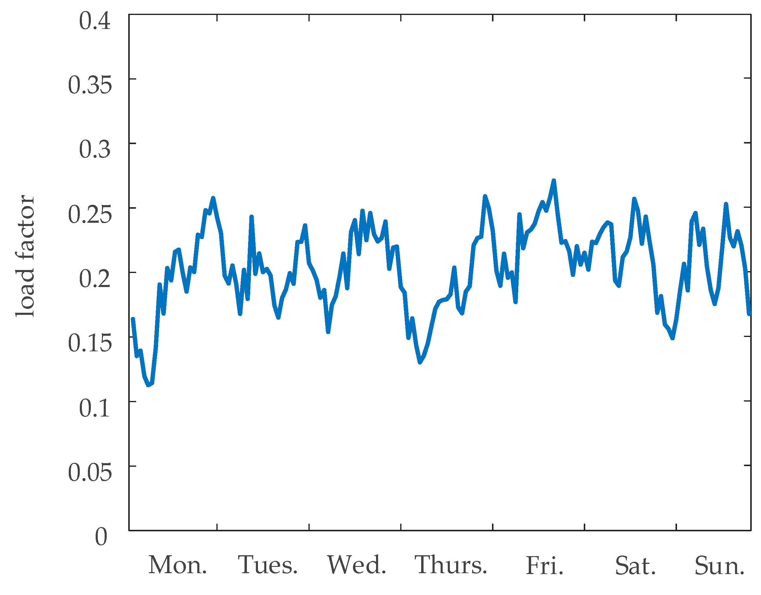
The component matrix after rotation is shown in

Table 5. Rotated component matrix.

Common Factor	Ambient Temperature	Load Current	Top Oil Temperature
1	0.913	0.376	0.796
2	0.313	0.922	0.497

. Obviously, the first common factor corresponds to a larger value in terms of ambient temperature and top oil temperature, while the second common factor is associated with a higher value of load current compared to the other two factors, which better represents the characteristic parameter of load current. Therefore, the first common factor is known as temperature factor f₁, and the second common factor is known as load factor f₂. These factors primarily represent the temperature variables and load variables that impact the temperature rise characteristics of the transformer.

Table 6. Component score coefficient matrix.

Common Factor	Ambient Temperature	Load Current	Top Oil Temperature
1	0.889	−0.576	0.508
2	−0.503	1.267	−0.021

shows the component score coefficient matrix after the rotation factor. Factor scores corresponding to temperature factor f1 and load factor f2 are obtained. They are entered into the fully connected neural network as two new variables.

$$\{\begin{array}{l}{f}_1=0.889\stackrel{⌢}{x_1}-0.576\stackrel{⌢}{x_2}+0.508\stackrel{⌢}{x_3}\\ f_2=-0.503\stackrel{⌢}{x_1}+1.267\stackrel{⌢}{x_2}-0.021\stackrel{⌢}{x_3}\end{array}$$

(7)

where $\stackrel{⌢}{x_1}$, $\stackrel{⌢}{x_2}$, and $\stackrel{⌢}{x_3}$ are the three original variables after standardization.

4.3. Case Verification

(1)

Parameter setting:

Based on the above preprocessing, two factor scores are obtained after factor analysis. Therefore, the input layer node of the network is set to 2; the output of the network is the AWTT predicted with the model, so the output layer node of the network is set to 1. The number of hidden layers and the number of nodes are dynamically altered and determined based on the actual situation. In order to guarantee the precision and effectiveness of the network model, the number of hidden layers is 1 and the number of nodes in each layer is 6 by debugging the network model.

In the training process, 70% of the sample data constitute the model training set, and 15% of the sample data are set aside to constitute the verification set. Adjust model parameters and preliminarily evaluate model capabilities. Then, 15% of the sample data are used as a test set to evaluate the generalization ability of the final model.

In order to show the validity of the model, the root mean square error (RMSE) and goodness of fit (R²) of the model prediction are selected as the indexes to evaluate the accuracy of the model prediction results. RMSE is the square root of the square of the difference between the predicted value and the actual value of the sample and the ratio of the number of samples, which can characterize the difference between the predicted value and the real value of the sample.

$$RMSE=\sqrt{{\displaystyle \frac{{\displaystyle \sum _{i=1}^n{(y-\widehat{y})}^2}}{n}}}$$

(8)

where R² describes how well the data fit the model and characterizes the regression fitting effect.

$$R^2=1-{\displaystyle \frac{{\displaystyle \sum _{i=1}^n{(y-\widehat{y})}^2}}{{\displaystyle \sum _{i=1}^n{(y-\overline{y})}^2}}}$$

(9)

where y is the measured value, $\widehat{y}$ is the predicted value, and $\overline{y}$ is the average value.

(2)

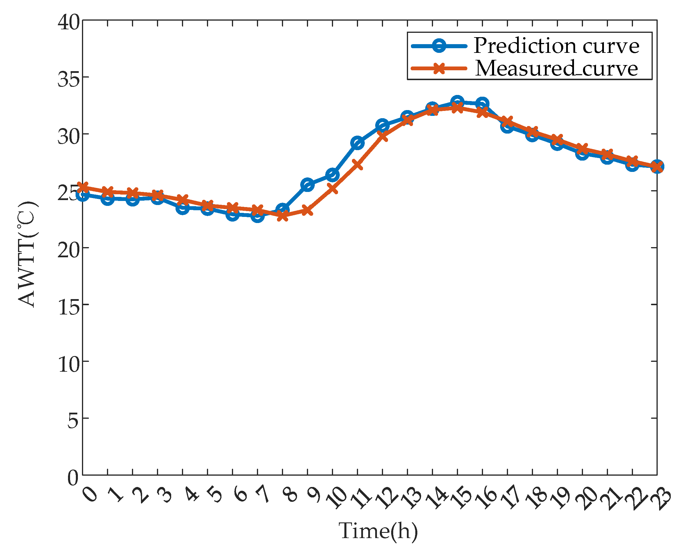
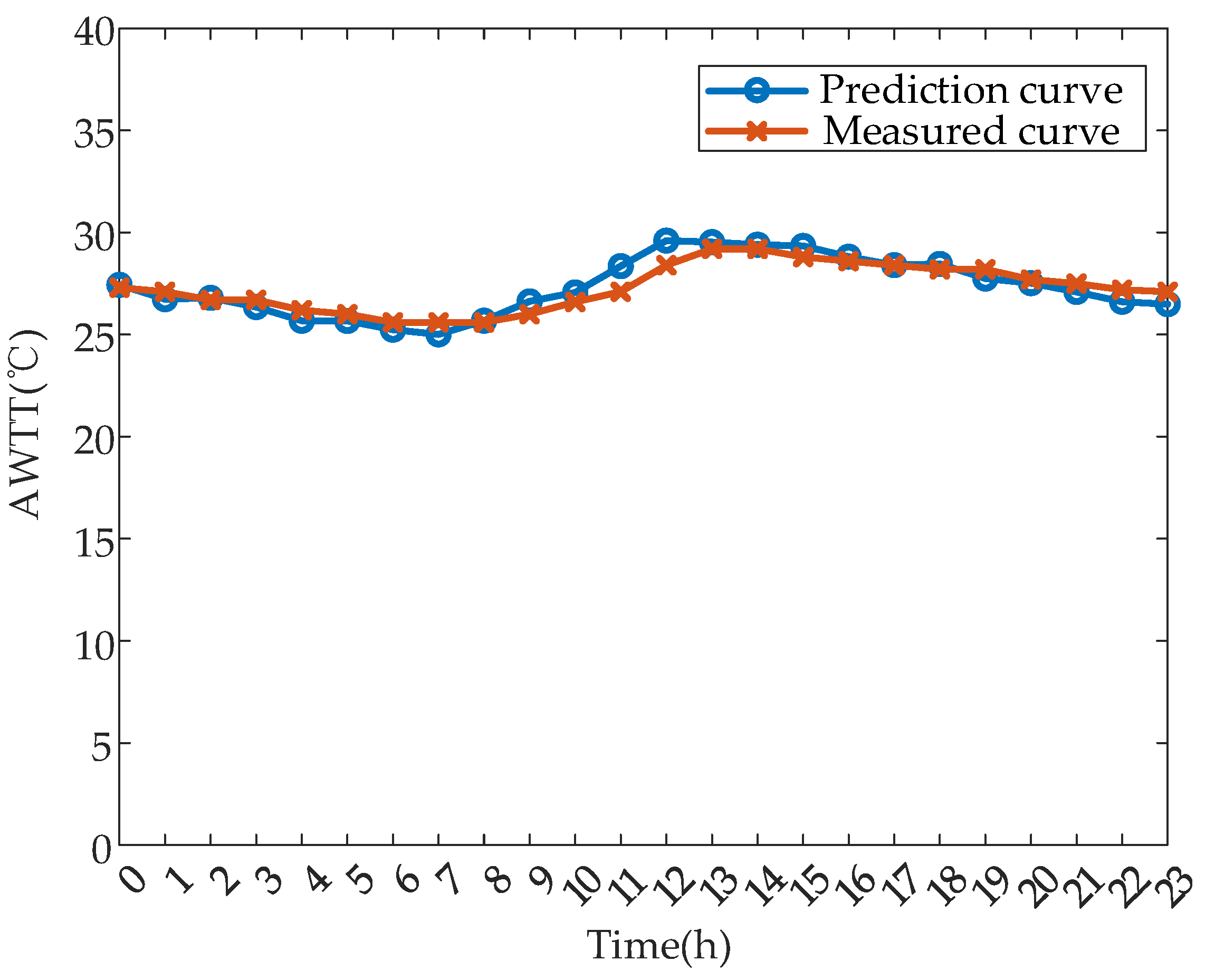
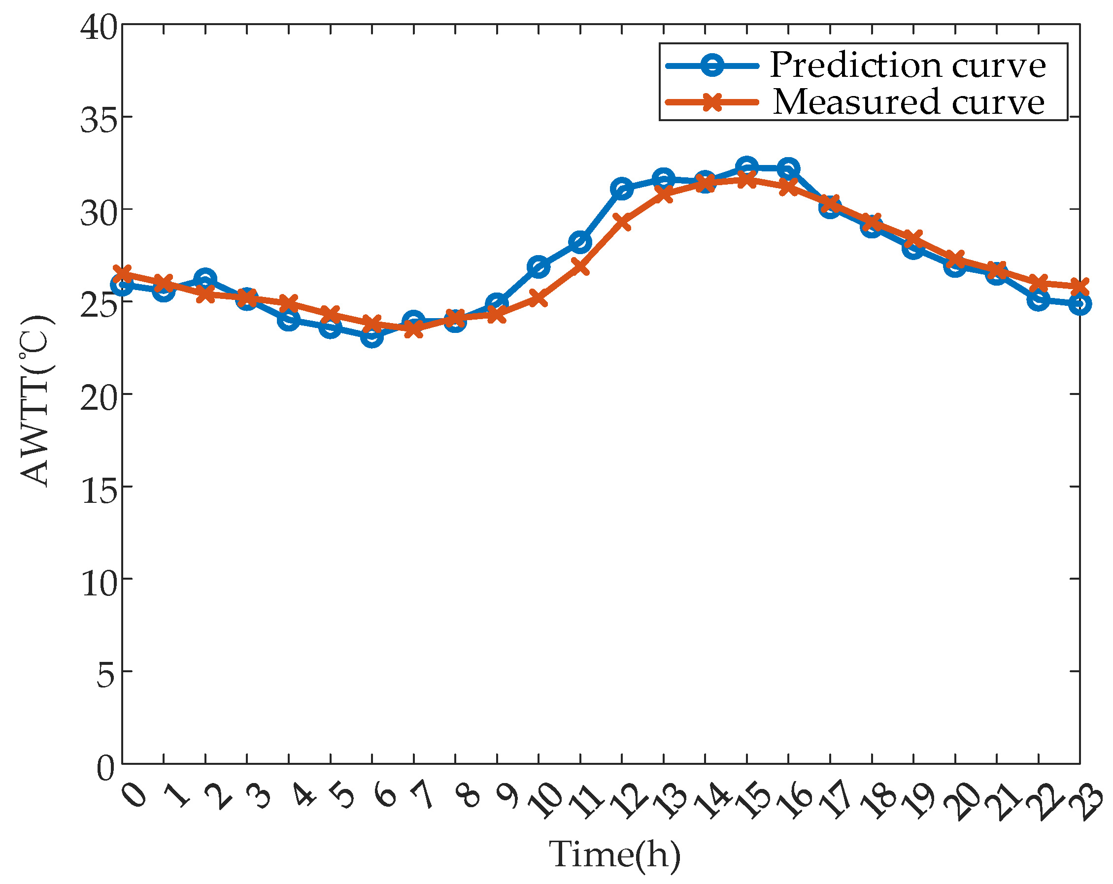
Results analysis:

Figure 8 shows the results of the AWTT curve measured in the field and predicted with the method in this paper. It can be seen from the diagram that the predicted curve is basically consistent with the actual curve. Further calculation shows that the RMSE between the predicted result and the actual value of AWTT is 0.62498, the R² is 0.9714, the average error is 0.6037 °C, and the maximum error percentage is 2.23%. That is, the average difference between the predicted result and the actual value is small, and the actual value can be well fitted.

The prediction results obtained with this method are basically consistent with the actual measured AWTT change trend. Among them, the AWTT corresponding to the daytime is higher, and the AWTT at night is reduced, which is consistent with the actual situation. The daytime is the peak period of electricity consumption every day. Especially from 9:00 to 17:00, the demand for the power grid is large. The transformer will bear a large load, and the load current will increase accordingly. The current in the primary and secondary transformer windings increases, resulting in a large amount of copper consumption in the coil resistor made of copper wire. The main heat sources during the operation of the transformer are iron core loss and winding loss. The increase in copper loss leads to more energy inside the winding to be converted into heat energy. This heat will first be transmitted to the winding and transformer oil in the form of heat conduction, affecting the AWTT and oil temperature. Heat is emitted from the outer wall of the fuel tank to the air through convective heat dissipation and thermal radiation. The expression between the heat and the temperature rise of the natural convection of the air, and the expression between the heat radiated from the tank wall to the air and the ambient temperature, are provided in (10) and (11).

$$\varphi =Sh(T_w-T_h)$$

(10)

$$\varphi =\sigma ES(T_w^4-T_h^4)$$

(11)

where $S$ is the surface area, $h$ is the convective heat transfer coefficient, $T_w$ is the outer surface temperature of the transformer tank, $T_h$ is the ambient temperature, $\sigma$ is the Stephen–Boltzmann constant, and $E$ is the surface radiation coefficient.

The greater the difference between the temperature of the oil tank wall and the ambient temperature, the more conducive it is for heat dissipation of the oil-immersed transformer to reduce the internal temperature. In most cases, 9:00 to 17:00 is a period of high temperature in the day. The temperature difference between the transformer tank and the surrounding air medium is small. The heat emitted into the air can be reduced accordingly, affecting the heat dissipation effect of the transformer. During this period, the AWTT is higher. On the contrary, in the low-power period with smaller load, that is, late at night and early in the morning, the corresponding heat generation is reduced, and the heat dissipation is increased. The AWTT during this period is relatively reduced.

Figure 9 and Figure 10 show the prediction curves when the AWTT fluctuates more gently and more frequently. The error corresponding to different fluctuations of the AWTT is shown in

Table 7. Error results under different fluctuations of the AWTT.

	Gentle Fluctuation	Moderate Fluctuation	Frequent Fluctuation
RMSE	0.2696	0.6250	0.6441
MAE	0.399	0.6037	0.6263
MAPE	1.47%	2.31%	2.33%

. The results show that the proposed method can achieve better temperature prediction in the case of gentle, moderate, and frequent fluctuation of the AWTT. It has good accuracy and reliability and meets the requirements for data quality in state assessment.

(3)

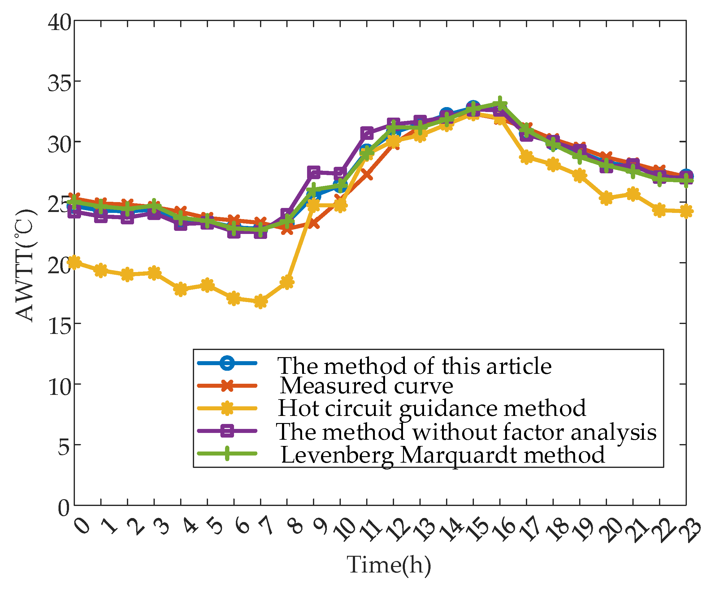
Comparative analysis

To further show the effectiveness and superiority of the proposed method, the results of the thermal circuit guidelines, the results obtained with factor analysis of the original data, and the results obtained by using the Levenberg–Marquardt (L-M) method to train the network are compared with the actual measured values. The results are shown in Figure 11 and Figure 12 and

Table 8. Accuracy evaluation table corresponding to different methods.

	Textual Method	Hot Circuit Guide Method	Method without Factor Analysis	L-M Method
RMSE	0.6250	14.7216	1.9175	0.8253
MAE	0.6027	3.1368	0.9761	0.6819
MAPE	2.31%	12.40%	3.79%	2.58%
R2	0.9714	0.1835	0.8474	0.9563

. Obviously, the prediction results obtained with the proposed method are optimal in terms of RMSE, mean absolute error (MAE), mean absolute percentage error (MAPE), R², and absolute error compared with the results of other methods mentioned above. As a result, the proposed method can achieve more accurate prediction of the AWTT considering that the fitting results are more accurate with the actual measured values. Among those methods, the error result of the thermal circuit guideline method is the largest, and the RMSE reaches 14.72164. The reason is that the method relies on empirical values. However, the oil index and rated oil time constant values used in the calculation process are difficult to accurately obtain. They can only be roughly estimated based on parameters such as transformer capacity level, and the accuracy in reflecting the existing performance of transformers and the degree of oil aging is limited. There are errors between the actual values, resulting in significant deviations between the final results and the measured values. Since the L-M method uses error minimization for optimization, in a nonlinear network with multiple local minimums, it is easily trapped in the local minimum and it may not be able to achieve the global minimum, thus affecting the generalization ability of the network. The RMSE of the L-M algorithm increases by 0.2003 compared with the Bayesian regularization algorithm used in this paper. By comparing the results of the factor analysis algorithm for original variables with or without factor analysis, the accuracy of the result is significantly improved compared with the hot path guide method, although it is not preprocessed with factor analysis. However, when comparing the findings after factor analysis preprocessing, there are still issues of significant inaccuracies and inaccurate accuracy. When there is a strong correlation between input variables, the possibility of multicollinearity and redundant data contained in it increases. As a result, the network may be unable to accurately confirm the independent impact of each variable on the output. What is more, the network model becomes overly reliant on specific features and overfits the correlation, leading to the problem of network overfitting. Specifically, the network model is too complex to fit the correlation relationship in the training data, and cannot flexibly adapt to the new data, thus reducing the final prediction accuracy.

The absolute error results show that the maximum error between the predicted AWTT and the field measured value occurs from 9:00 to 12:00, and the maximum absolute error is 2.22 °C, 4.17 °C, and 2.74 °C, respectively, when based on the proposed method, the method without using factor analysis, and the L-M method. This period can be like the start-up process of the transformer. The corresponding load is stable in the late night and early morning periods, and it is approximately considered that the AWTT and the oil temperature are balanced and in a stable state. From 8:00 to 9:00, the load will change and fluctuate greatly, in contrast to the previous period. In addition, the load current increases and the AWTT rises. The external insulating oil is expanded by the heating volume, and the upward convection is carried out. At the same time, due to the large internal temperature difference, the winding heat dissipation accelerates and reaches the heat balance state faster. However, the transformer fails to achieve a thermal steady state, leading to fluctuations in its temperature. It keeps rising until it reaches the quasi-steady state. Currently, due to the large heat capacity of the transformer, the internal heat dissipation and heat generation are not equal, resulting in continuous temperature changes. Once the transformer reaches the thermal steady state, its temperature will remain relatively constant. The whole process is relatively slow and takes a long time. From 9:00 to 12:00, the winding is in a stage in which it has not yet reached a stable state, leading to a significant prediction inaccuracy during this period. After 12:00, the error between the predicted AWTT and the measured value noticeably decreases, and the maximum absolute error does not exceed 0.75 °C, indicating a strong agreement with the measured value.

Considering the relevant evaluation indicators and results, it can be considered that the prediction curve obtained with the method proposed in this paper is closer to the actual measured value, and the overall effect is better than the thermal path guideline method, the L-M method, and the method without factor analysis preprocessing, which verifies the effectiveness of the method proposed in this paper. In practical applications, the current operating state of the transformer can be determined, based on the difference between the temperature prediction value of the proposed method and the actual value of the current AWTT feedback from the sensor. If the difference is too large, it indicates that there is a problem with the operation of the transformer, or an abnormal value has occurred.

5. Discussion and Conclusions

A prediction model based on a fully connected neural network is proposed, which can predict the AWTT accurately. In order to remove the coupling among the original imputs and improve the efficiency of the network model, the factor analysis algorithm is used. Furthermore, without reducing the prediction accuracy of the AWTT, less data are used to reduce the dimension of data processing. The conclusions are as follows:

(1)

After factor analysis is adopted, the coupling among ambient temperature, load current, and top oil temperature can be effectively removed. Two key parameters, the temperature factor and load factor, are proposed to reduce the complexity of the network model, which reduces the amount of data input and improves the efficiency;

(2)

The prediction model based on factor analysis and a fully connected neural network can accurately obtain the AWTT. The RMSE between the predicted results and the measured values of the AWTT is 0.62498, and the R² is 0.9714, which shows the feasibility of the proposed method;

(3)

Compared with the thermal circuit guideline method, the L-M method and the method without factor analysis, the results show that the prediction method proposed in this paper has higher accuracy and reliability. Combined with the predicted results, the abnormal values can be removed and corrected to make the AWTT prediction more accurate, which is of great significance for the prediction of the winding hot-spot temperature and transformer state assessment.

On the basis of collecting historical state data of transformers, the proposed method can be applied to establish a unique and accurate AWTT prediction model for each transformer. It helps to fully analyze and mine monitoring data, promoting the development of the power supply system from maintenance after faults and planned maintenance to maintenance based on transformer state. This can detect safety hazards in advance, improve operation and maintenance efficiency, and reduce costs. In addition, further research will be conducted on transformers of different voltage levels and models, to improve the applicability of the method proposed in this paper.

References

- Yuan, F.T.; Yang, W.T.; Han, Y.L. Temperature Rise Calculation and Structure Optimization Research of Transformer Winding Based on Electromagnetic-fluid-thermal Coupling. High Volt. Eng. 2024, 50, 952–961. [Google Scholar]
- Yao, S.; Hao, Z.; Si, J.; Zhang, Y. Dynamic deformation analysis of power transformer windings under multiple short-circuit impacts. In Proceedings of the IEEE 8th International Conference on Advanced Power System Automation and Protection (APAP), Xi’an, China, 21–24 October 2019; pp. 1394–1397. [Google Scholar]
- Qiu, Z.; Ruan, J.; Huang, D.; Wei, M.; Tang, L.; Huang, C.; Xu, W.; Shu, S. Hybrid prediction of the power frequency breakdown voltage of short air gaps based on orthogonal design and support vector machine. IEEE Trans. Dielectr. Electr. Insul. 2016, 23, 795–805. [Google Scholar] [CrossRef]
- Ni, Z.Z.; Luo, Y.T.; Jiang, J.F. Multi-timescale Prediction of Transformer Top Oil Temperature Based on Adaptive Extended Kalman Filter. Power Syst. Technol. 2024, 1–11. [Google Scholar]
- Wang, L.J.; Zhou, L.J.; Yuan, S. Improved dynamic thermal model with pre-physical modeling for transformers in ONAN cooling mode. IEEE Trans. Power Deliv. 2019, 34, 1442–1450. [Google Scholar] [CrossRef]
- Li, H.; Liu, Y.P.; Wang, J.X. Analysis and Test Verification of Dynamic Thermal Model of Oil-immersed Distribution Transformer. Proc. CSEE 2023, 43, 389–399. [Google Scholar]
- Farzin, N.; Vakilian, M.; Hajipour, E. Practical implementation of a new percentage-based turn-to-turn fault detection algorithm to transformer digital differential relay. Int. J. Electr. Power Energy Syst. 2020, 121, 106158. [Google Scholar] [CrossRef]
- Sönmez, O.; Komurgoz, G. Determination of hot-spot temperature for ONAN distribution transformers with dynamic thermal modelling. In Proceedings of the 2018 Condition Monitoring and Diagnosis (CMD), Perth, Australia, 23–26 September 2018; pp. 1–9. [Google Scholar]
- C57.91-2011; IEEE Guide for Loading Mineral-Oil-Immersed Transformers and Step-Voltage Regulators. IEEE: Piscataway, NJ, USA, 2011.
- IEC 60076-7: 2018; Power Transformers-Part 7: Loading Guide for Mineral-Oil-Immersed Power Transformers. American National Standards Institute (ANSI): New York, NY, USA, 2018.
- Swift, G.; Molinski, T.S.; Lehn, W. A fundamental approach to transformer thermal modeling. I. Theory and equivalent circuit. IEEE Trans. Power Deliv. 2001, 16, 171–175. [Google Scholar] [CrossRef]
- Nordman, H.; Rafsback, N.; Susa, D. Temperature responses to step changes in the load current of power transformers. IEEE Trans. Power Deliv. 2003, 18, 1110–1117. [Google Scholar] [CrossRef]
- Liao, C.B.; Ruan, J.J.; Lu, H.D. 2-D Coupled Electromagnetic-fluid-thermal Analysis of Oil-immersed Transformer. Sci. Technol. Eng. 2014, 14, 67–71. [Google Scholar]
- Wang, Y.Q.; Ma, L.; LV, F.C. Calculation of 3D Temperature Field of Oil Immersed Transformer by the Combination of the Finite Element and Finite Volume Method. High Volt. Eng. 2014, 40, 3179–3185. [Google Scholar]
- Li, T.; Sun, X.W.; Du, X.P. Simulation Analysis of Transformer Flow Field and Temperature Field Based on Finite Element Method. Autom. Instrum. 2020, 35, 1–5+10. [Google Scholar]
- Li, K.J.; Qi, X.W.; Wei, B.G. Prediction of Transformer Top Oil Temperature Based on Kernel Extreme Learning Machine Error Prediction and Correction. High Volt. Eng. 2017, 43, 4045–4405. [Google Scholar]
- Li, K.J.; Xu, Y.S.; Wei, B.G. Prediction Model for Top Oil Temperature of Transformer Based on Hybrid Kernel Extreme Learning Machine Trained and Optimized by Particle Swarm Optimization. High Volt. Eng. 2018, 44, 2501–2508. [Google Scholar]
- Zhang, Y.Y.; Wei, X.X.; Fan, X.H.; Wang, K.; Zhuo, R. A Prediction Model of Hot Spot Temperature for Split-Windings Traction Transformer Considering the Load Characteristics. IEEE Access 2021, 9, 22605–22615. [Google Scholar] [CrossRef]
- Yang, J.J.; Zhang, G.; Liu, Y.F.; Gong, Z.F.; Liu, Z.G. A method for calculating hot-spot temperature of traction transformer based on multi-physical model and combined neural network. IEEE Trans. Transp. Electrif. 2023. [Google Scholar] [CrossRef]
- Wei, B.G.; Wu, X.Y.; Yao, Z.F.; Huang, H. A method of optimized neural network by L-M algorithm to transformer winding hot spot temperature forecasting. In Proceedings of the IEEE Electrical Insulation Conference (EIC), Baltimore, MD, USA, 11–14 June 2017; pp. 87–91. [Google Scholar]
- Peng, D.G.; Chen, Y.W.; Qian, Y.L.; Huang, C. Transformer Winding Temperature Soft Measurement Model Based on Particle Swarm Optimization-Support Vector Regression. Trans. China Electrotech. Soc. 2018, 33, 1742–1749. [Google Scholar]
- Chegsakul, T.; Tayjasanant, T. An impact of harmonic currents, load levels and ambient temperatures on transformer loss of life. J. Phys. Conf. Ser. 2019, 1311, 012047. [Google Scholar] [CrossRef]
- Luo, C.; Zhao, Z.G.; Wang, Y.Y.; Liang, K.; Zhang, J.H.; Li, Y.N.; Li, C. Influence of insulation paper on the hot spot temperature of oil-immersed transformer winding. Mod. Phys. Lett. B 2022, 35, 2140021. [Google Scholar] [CrossRef]
- Gorgan, B.; Notingher, P.V.; Wetzer, J.M.; Verhaart, H.F.A.; Wouters, P.A.A.F.; Van Schijndel, A. Influence of solar irradiation on power transformer thermal balance. IEEE Trans. Dielectr. Electr. Insul. 2012, 19, 1843–1850. [Google Scholar] [CrossRef]