Adaptive Truncation Threshold Determination for Multimode Fiber Single-Pixel Imaging

Abstract

Truncated singular value decomposition (TSVD) is a popular recovery algorithm for multimode fiber single-pixel imaging (MMF-SPI), and it uses truncation thresholds to suppress noise influences. However, due to the sensitivity of MMF relative to stochastic disturbances, the threshold requires frequent re-determination as noise levels dynamically fluctuate. In response, we design an adaptive truncation threshold determination (ATTD) method for TSVD-based MMF-SPI in disturbed environments. Simulations and experiments reveal that ATTD approaches the performance of ideal clairvoyant benchmarks, and it corresponds to the best possible image recovery under certain noise levels and surpasses both traditional truncation threshold determination methods with less computation—fixed threshold and Stein’s unbiased risk estimator (SURE)—specifically under high noise levels. Moreover, target insensitivity is demonstrated via numerical simulations, and the robustness of the self-contained parameters is explored. Finally, we also compare and discuss the performance of TSVD-based MMF-SPI, which uses ATTD, and machine learning-based MMF-SPI, which uses diffusion models, to provide a comprehensive understanding of ATTD.

1. Introduction

Multimode fibers (MMFs) are expected extensions of fiber bundles [1,2,3,4,5,6], and examples include endoscopic probes [7,8]. However, mode coupling and dispersion scramble transmitted images into unrecognizable speckles, rendering direct imaging impossible. Therefore, several methods have been developed for MMF imaging, such as (1) wavefront shaping-based raster scanning [9,10,11,12]; (2) single-pixel imaging (SPI [13] or, equivalently, ghost imaging [14]); and (3) machine learning [15,16,17,18]. Wavefront shaping requires complex interference setups to measure transmission matrices for characterization of MMF transmission and to control the output of scanned point-by-point MMF objects. Machine learning methods leverage large datasets to train models that can reconstruct images from speckle patterns and require extensive training data. In MMF-SPI [19,20,21,22,23,24,25,26,27,28], MMF is used as a light projector to illuminate the target; then, the light intensity response of the target is recorded. With the help of SPI algorithms, the image can be recovered [29]. Compared with raster scanning and machine learning methods, SPI has advantages in terms of simplicity compared to wavefront shaping because only light intensity is required, avoiding interference setups; it also has advantages in terms of imaging speeds compared to machine learning because a few measurements are enough.

Compared with conventional SPI, MMF-SPI is more susceptible to stochastic noise; thus, not all SPI algorithms work. A linear correlation method such as second-order correlation is a simple and quick SPI algorithm, relying on the orthogonality of the measurement matrix, but it often performs poorly in practical MMF-SPI [21,24] because the measurement matrix derived from MMF speckle patterns typically has lower orthogonality than assumed. Regularized optimization methods such as compressive sensing (CS) [19,20,21,22,23,24] can provide better image quality through the fine tuning of regularized parameters. However, this key parameter can only be empirically specified beforehand or is gradually found via costly iterations, ruling out high-speed imaging. For machine learning, the acquisition of large-scale data, model training, and parameter fine tuning are inevitable [30]. In terms of balancing costs, performance, and robustness, the relatively old truncated singular value decomposition (TSVD) still enjoys unique advantages. Computing the pseudo-inverse of measurement matrices with a suitable truncation threshold to maintain image information and suppress noise at the same time, TSVD has become popular with MMF-SPI [25,26,27,28]. However, MMF-SPI is fragile relative to disturbances [31,32,33,34,35,36] such as fiber bending, resulting in dynamical changes in noise levels and, thus, requiring a flexible truncation threshold for recovery.

When complete knowledge of the target is known, it is possible to test all potential truncation thresholds to identify the optimal one, which is known as the clairvoyant benchmark. This benchmark minimizes the recovery error and serves as a reference for truncation threshold selection. In practice, this critical truncation threshold can be chosen without prior knowledge via traditional methods such as the L-curve [37] and generalized cross-validation (GCV) [38,39] methods. The L-curve method selects the truncation point at the curve’s corner, and it is plotted as the norm of the solution against the norm of the residual. GCV selects the threshold by minimizing the cross-validation error. The computational complexity of both methods is related to the square of the pixel number, rendering them unsuitable for high-speed imaging applications, especially in disturbed conditions requiring frequent re-determination. For more efficient methods with less computation, fixed truncation and Stein’s unbiased risk estimator (SURE) [40] are recommended. The former selects truncation thresholds directly via the singular value (SV) spectrum [25,26,27,28]. The latter is believed to be the state of the art for threshold noise signals. Unfortunately, both show a low correlation with the recovered image of the benchmark threshold as noise increases.

This study aims to develop an adaptive truncation threshold determination (ATTD) method for TSVD-based MMF-SPI in disturbed environments, aiming to improve image quality under various noise levels. Simulations and experiments suggest that ATTD can approach the clairvoyant benchmark, which represents the upper bound of performance achievable with prior knowledge of the target. Even under high-noise conditions where fixed truncation thresholds and SURE are less effective, the ATTD method exhibits robust performance. Additionally, the ATTD parameters are self-determined, and their stability is examined. The unique aspects of this work include the adaptive nature of the thresholding mechanism, which adjusts to varying noise levels without requiring prior knowledge, and the notable improvements in image recovery under high-noise conditions, offering a potentially robust solution for real-time applications.

2. Method

2.1. Background: Measurement and Recovery

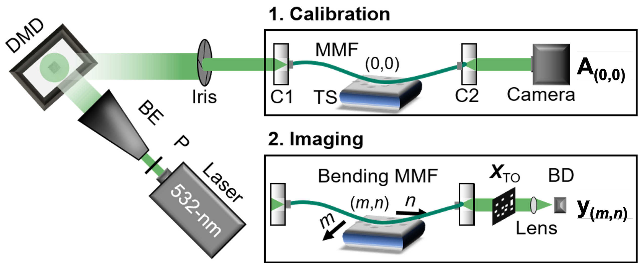
2.1.1. Measurement of Multimode Fiber Single-Pixel Imaging (MMF-SPI)

Figure 1 shows the measurement procedure of MMF-SPI. With random input modulations, MMF consecutively shines speckles on a target ($\mathbf{x}$). Transmitted light is collected with a focus lens and registered as a light intensity sequence ($\mathbf{y}$) via a bucket detector (BD), which has no spatial resolution. Ideally, the noise-free BD signal reads $\mathbf{y}$ = $\mathbf{Ax}$, where each speckle is previously recorded using an array detector and shaped as a row of a measurement matrix ($\mathbf{A}$). The target ($\mathbf{x}$) is reshaped into a column vector. Generally, $\mathbf{A}$ is fixed for recovery after previous captures. Therefore, disturbances such as MMF bending cause illumination deviations ($▵\mathbf{A}$), resulting in a mismatch between $\mathbf{A}$ and ${\mathbf{y}}_{\mathrm{disturbed}}=(\mathbf{A}+▵\mathbf{A})\mathbf{x}$. With noise, the BD signal is $\mathbf{y}+\mathbf{e}$ instead, where the term $\mathbf{e}$ includes the following two parts: (1) mismatch noise ($▵\mathbf{A}\mathbf{x}$) and (2) initially electric BD noise. The noise level of $\mathbf{e}$ changes dynamically via unavoidable disturbance. Here, we assume that both types of noises can be modeled via Gaussian noise. The rationale for the impact of Gaussian equivalence on bending is discussed in Section 4.

2.1.2. Recovery via Truncated Singular Value Decomposition (TSVD)

As a common solution to the inverse problem, TSVD utilizes a truncation threshold ($\mathit{k}$) to obtain the Moore–Penrose inverse of $\mathbf{A}$ (${\mathbf{A}}_{\mathit{k}}^{†}$). Then, the target ($\mathbf{x}$) can be restored as follows:

$${\widehat{\mathbf{x}}}_k={\mathbf{A}}_k^{†}(\mathbf{y}+\mathbf{e})=\sum _{j=1}^k{\displaystyle \frac{{\mathbf{u}}_j^{\mathsf{T}}(\mathbf{y}+\mathbf{e}){\mathbf{v}}_j}{{\mathbf{s}}_j}},1\le k\le N_{\mathrm{mea}},$$

(1)

where column vectors ${\mathbf{u}}_j$ and ${\mathbf{v}}_j$, together with the corresponding SV (${\mathbf{s}}_j$), are obtained via the singular value decomposition (SVD) of $\mathbf{A}$, i.e., $\mathbf{A}={\mathbf{USV}}^{\mathsf{T}}$. ${\mathbf{u}}_j$ and ${\mathbf{v}}_j$ are the columns of orthogonal matrices $\mathbf{U}$ and $\mathbf{V}$, respectively. $\mathbf{S}=\mathsf{diag}\left\{{\mathbf{s}}_j\right\}$ contains all SVs. Truncation (k) limits the measurement number ($N_{\mathrm{mea}}$). Recovery involves solving an inverse problem to obtain $\widehat{\mathbf{x}}$ from $\mathbf{A}$ and $\mathbf{y}+\mathbf{e}$. The negative values of ${\widehat{\mathbf{x}}}_k$ are set to zero due to the physical nature of the images.

As Equation (1) shows, assuming that stochastic noise ($\mathbf{e}$) affects each vector (${\mathbf{u}}_j$) homogeneously, those with a smaller weight (${\mathbf{s}}_j$) would have a worse signal-to-noise ratio due to the amplification of $1/{\mathbf{s}}_j$, introducing more unwanted effects on the result. Thus, it is important to cut off at a certain threshold (k) in order to abandon components with smaller SVs [41].

2.2. Proposed Method: Adaptive Truncation Threshold Determination (ATTD)

The ATTD method begins with the assumption that the absolute value decomposition ($|{\mathbf{U}}^{\mathsf{T}}\mathbf{y}|$) generally follows a descending order, consistent with the SV distribution. However, the presence of noise disrupts this order, causing $|{\mathbf{U}}^{\mathsf{T}}(\mathbf{y}+\mathbf{e})|$ to become randomly distributed beyond a certain index. Therefore, the point at which the order is disrupted between the decomposition indices and the SV indices serves as a reference for distinguishing between signals and noise.

As the ATTD pseudo-code (Algorithm 1) shows, by inputting the noisy BD signal ($\mathbf{y}+\mathbf{e}$), the left singular matrix ($\mathbf{U}$) via the SVD of the recorded measurement matrix ($\mathbf{A}$), and the self-contained VAR and TOL parameters, the threshold ($k_{\mathrm{d}}$) is determined. Note that VAR and TOL can be calibrated independently via several numerical simulations using only the measurement matrix ($\mathbf{A}$), as described in Appendix A (Algorithms A1 and A2, respectively). Each step is described as follows:

(1)

Projection: Calculate the absolute value of decomposition coefficients ($\mathbf{c}=|{\mathbf{U}}^{\mathsf{T}}(\mathbf{y}+\mathbf{e})|$).

(2)

Sorting: Sort sequence $\mathbf{c}$ in descending order to obtain ${\mathbf{c}}_{\mathrm{sorted}}$ and the corresponding index ($\mathbf{i}$).

(3)

Binary transformation: Apply a naïve test function to binary $|k-{\mathbf{i}}_k|$ as follows:

$${\mathbf{b}}_k=\left\{\begin{array}{cc}0,\hfill & \mathrm{if}|k-{\mathbf{i}}_k|>\mathrm{VAR}\hfill \\ 1,\hfill & \mathrm{otherwise}\hfill \end{array}\right.$$

(2)

(4)

Accumulated average: Compute the accumulated average of the first k values of $\mathbf{b}$ as follows:

$${\mathbf{ave}}_k={\displaystyle \frac{1}{k}}\sum _{j=1}^k{\mathbf{b}}_j,1\le k\le N_{\mathrm{mea}},$$

(3)

where the ${\mathbf{ave}}_k$ sequence generally decreases with k.

(5)

Determination: Determine the truncation threshold $k_{\mathrm{d}}$ via the maximum index when the accumulated average ($\mathbf{ave}$) is larger than a certain proportion of its maximum, i.e., $\mathrm{TOL}·\max \left(\mathbf{ave}\right)$.

$$k_{\mathrm{d}}=max\left\{k\mid {\mathbf{ave}}_k\ge \mathrm{TOL}·max\left(\mathbf{ave}\right),1\le k\le N_{\mathrm{mea}}\right\}.$$

(4)

Algorithm 1 $k_{\mathrm{d}}=$ ATTD$(\mathbf{y}+\mathbf{e},\mathbf{U},\mathrm{VAR},\mathrm{TOL}$)

1: function ATTD($\mathbf{y}+\mathbf{e},\mathbf{U},\mathrm{VAR},\mathrm{TOL}$)   2:     $\mathbf{c}\leftarrow \left|{\mathbf{U}}^{\mathsf{T}}(\mathbf{y}+\mathbf{e})\right|$; ▹ (1) Project step.   3:     $\mathbf{i}\leftarrow \mathrm{sort}\left(\mathbf{c}\right)$;▹ (2) Sort $\mathbf{c}$ in descending order and obtain corresponding indexes.   4:     for $k\leftarrow 1$ to $k\leftarrow$ length($\mathbf{i}$) do   5:         compute ${\mathbf{b}}_k$ via Equation (2); ▹ (3) Naïve test function to sift $|k-{\mathbf{i}}_k|$.   6:         compute ${\mathbf{ave}}_k$ via Equation (3); ▹ (4) Accumulated average.   7:     end for   8:     compute $k_{\mathrm{d}}$ via Equation (4); ▹ (5) Determination.   9:     return $k_{\mathrm{d}}$ 10: end function

2.3. Experimental Design, Implementation, and Evaluation

2.3.1. Overall Experimental Design

To validate the effectiveness of ATTD, we designed the following experiments:

(1)

Adaptation to varying noise levels: First, we conducted imaging experiments using both simulated BD sequences with adjustable noise levels and real BD sequences disturbed by a bending MMF to verify adaption to noise variations in ATTD. For the results, please refer to the first two parts of Section 3. Note that we assume that the noise generated via fiber bending in MMF-SPI is equivalent to the Gaussian additive noise added in BD sequences. The rationale for this approximation is explained in Section 4.

(2)

Target insensitivity: Secondly, due to experimental constraints, we conducted experiments on simulated BD sequences generated from different targets (USC-SIP image database containing 210 images [42]) with varying noise levels to verify the object insensitivity of ATTD. For the results, please refer to the third part of Section 3.

(3)

Stability of the TOL parameters: Finally, we investigated whether the self-contained TOL parameters calibrated with one measurement matrix are applicable to other measurement matrices. For the results, please refer to the forth part of Section 3.

2.3.2. Implementation of Dynamically Changing Noise Levels

To verify the adaptation capability of ATTD, two methods were adopted to dynamically change noise levels in simulations and realistic experiments.

First, the measurement matrix should be obtained via realistic calibration, as shown in Figure 2. Polarized and expanded 532 nm coherent light was modulated by a digital micro-mirror device (DMD). Then, it was shaped by an iris and coupled into fibers via collimator C1. After transmission, an output speckle pattern was collimated via C2. Then, 2500 pseudo-random illumination patterns were consecutively captured by a CMOS camera and, finally, shaped into ${\mathbf{A}}_{(0,0)}$, where the sub-label represents the initial translation stage (TS) position. Note that the VAR and TOL parameters of ATTD were calibrated via simulations using ${\mathbf{A}}_{(0,0)}$. Here, TOL was set at 0.4 (refer to Appendix A).

Then, in simulation, the noisy simulated BD signal sequence (${\mathbf{y}}_{\mathrm{sim}}={\mathbf{A}}_{(0,0)}{\mathbf{x}}_{\mathrm{TO}}+\mathbf{e}\left(\mathrm{ratio}\right)$) was created by adding additive Gaussian noise with an adjustable ratio to the simulated BD signal (for details on the computation of the ratio, please refer to Algorithm A2 in Appendix A). Here, ${\mathbf{x}}_{\mathrm{TO}}$ depicts GI letters comprising pixelated blocks, as shown in Figure 3a.

Finally, in realistic imaging experiments, dynamical changes in noise levels were realized via TS movement. A transmissive mask corresponding to ${\mathbf{x}}_{\mathrm{TO}}$ was placed in front of the camera. The camera, functioning as a BD, captured transmitted light as a single-pixel sum. After the same modulations as for calibration, the BD signal was registered as a column vector ($\mathbf{y}$). Noise levels were manipulated by a bending MMF attached to TS, with various positions $(m,n)$ altering the noise level. Disturbed BD signals (${\mathbf{y}}_{(m,n)}$) could be recorded by moving TS, causing speckles (${\mathbf{A}}_{(m,n)}$) being shone on targets other than ${\mathbf{A}}_{(0,0)}$ as recorded in calibration. This illumination difference is equivalent to adding noise to a BD signal if it sticks to ${\mathbf{A}}_{(0,0)}$ for recovery. For endoscopy, only ${\mathbf{A}}_{(0,0)}$ could be obtained because ${\mathbf{A}}_{(m,n)}$ was inaccessible after MMF entered body. Therefore, the target is generally restored by the initial ${\mathbf{A}}_{(0,0)}$ and disturbed ${\mathbf{y}}_{(m,n)}$ (mismatch problem [21,35]).

2.3.3. Performance Evaluation via Clairvoyant Benchmark

To evaluate the performance of the proposed ATTD, the Pearson correlation between the recovered image and the clairvoyant benchmark was used, where the clairvoyant benchmark is the image restored via the clairvoyant truncation threshold ($k_{\mathrm{c}}$; refer to Algorithm A2 in Appendix A). $k_{\mathrm{c}}$ requires full knowledge of the target, which is obtained by iterating all truncation values to achieve the best image quality under a certain noise condition.

2.3.4. Comparative Truncation Threshold Determination Methods

First, we compared the recovery performance with traditional threshold methods. The following two methods with relatively low computational complexity were used: (1) fixed truncation ($k_{\mathrm{f}}$) and (2) Stein’s unbiased risk estimation (SURE). Fixed $k_{\mathrm{f}}$ was selected directly from the SVs using the index of SV that exceeds 1% of the maximum SV. The SURE requires some computations with knowledge of the noise level. In simulations, the known noise level was adopted for SURE calculations, while in practical experiments, the estimated noise level was used (for details about these two methods, please refer to Appendix B). We did not consider the L-curve and GCV methods in this comparison because their performances are close to that of the clairvoyant benchmark, which can be obtained iteratively, rendering their consideration unnecessary.

Secondly, we further considered two complex L-curve and GCV instances to compare the time–cost performance with respect to single recovery. Both methods achieved recovery performances approaching that of the clairvoyant benchmark and did not need a targeted prior. The procedure for the L-curve method is as follows: The residual ($|\mathbf{y}-\mathbf{A}{\mathbf{x}}_k{|}_2$) and solution norm ($|{\mathbf{x}}_k{|}_2$) are computed for each truncation (k), and the turning point on the plot of the residual versus solution norm is chosen. For GCV, the procedure involves calculating the generalized cross-validation score for each truncation (k) and selecting the k value that minimizes the GCV score ($\parallel \mathbf{y}-\mathbf{A}{\mathbf{x}}_k{\parallel }^2/{(N_{\mathrm{mea}}-k)}^2$). All data processing and experiments were conducted on a computer with the following specifications: Intel(R) Core(TM) i7-9750H CPU @ 2.60 GHz, 2.59 GHz, and 32 GB of RAM.

3. Results

3.1. Adapting Dynamical Noise Changes in Simulations

In the simulations, the proposed ATTD illustrated in the red box of Figure 3c maintained a high correlation relative to the clairvoyant benchmark reference across noise levels, with robustness measuring around −30 dB, outperforming the fixed truncation ($k_{\mathrm{f}}$) and SURE (as depicted in Figure 3d and Figure 3e, respectively). $k_{\mathrm{f}}$ achieved consistent but lower performance as noise increased, whereas SURE with a known noise ratio exhibited high fidelity at −70 dB but suffered a drastic performance decline at higher noise levels, indicating limited effectiveness in noisy environments.

3.2. Adapting the Dynamical Change in Noise in Practical Experiments

Figure 4 illustrates the adaption performance of ATTD across different noise conditions in an empirical setting, serving as a realistic validation for simulations. The top label $(m,n)$ denotes a distinct noise scenario (fiber configuration), and the clairvoyant benchmark in Figure 4a acts as an ideal reference under each noise level. The ATTD exhibited a high correlation with the clairvoyant benchmark shown in Figure 4b, with the performance only declining at the most severe bend (8, 8). In contrast, as Figure 4c shows, fixed truncation exhibited a decreasing trend with respect to correlation coefficients, which indicates a gradual deviation from the ideal reference with increasing noise. The last row reveals that SURE worked without fiber bending, and the limitations of SURE were observed when faced with severe bending. These empirical results corroborate with the simulation outcomes.

3.3. Adapting the Change in Simulated Targets

To show that ATTD generally works for different targets but is limited by experimental conditions, an image database (USC-SIP, containing 210 images [42]) was adopted. Each image was set as the target ($\mathbf{x}$) to produce simulated BD signals under different noise levels. As

Table 1. Average Pearson correlations relative to USC-SIP (${\mathbf{A}}_{(0,0)}$ and TOL = 0.4).

	−70 dB	−35 dB	−30 dB	−20 dB
ATTD	0.97	0.78	0.64	0.49
Fixed	0.93	0.51	0.34	0.14
SURE	0.63	0.03	0.02	0.02

shows, the proposed ATTD showed a strong correlation of 0.97 with the clairvoyant benchmark reference at −70 dB, decreasing with increased noise level and reaching a moderate correlation of 0.47 at −20 dB. Fixed truncation started with a high correlation of 0.93 at −70 dB, but it decreased significantly as noise increased, with a low correlation of 0.14 at −20 dB. SURE began with a moderate correlation of 0.63 at −70 dB and decreased sharply, reaching a negligible correlation at higher noise levels (−35 dB to −20 dB) and indicating a decline in performance in the presence of noise.

3.4. Robustness of TOL Parameter

According to the calibration methods for VAR and TOL provided in Appendix A, VAR was calibrated based on the specific measurement matrix, while TOL required a series of numerical simulations for calibration. Therefore, the stability of TOL is an important subject of study. To show that the choice of TOL is not affected by a different measurement matrix ($\mathbf{A}$), the following four groups of illumination speckle patterns captured under different fiber configurations were used: ${\mathbf{A}}_{(0,0)}$, ${\mathbf{A}}_{(0,24)}$, ${\mathbf{A}}_{(24,0)}$, and ${\mathbf{A}}_{(24,24)}$. Figure 5 shows that they are totally different, with very low Pearson correlation coefficients between them. Based on numerical simulations using the measurement matrix (${\mathbf{A}}_{(0,0)}$), we determined that TOL = 0.4. This value was then used in target-insensitivity simulations with different measurement matrices, the results of which are shown in the

Table 2. Average Pearson correlations relative to USC-SIP (different $\mathbf{A}$ and TOL = 0.4).

	−70 dB	−35 dB	−30 dB	−20 dB
${\mathbf{A}}_{(0,24)}$	0.98	0.77	0.63	0.48
${\mathbf{A}}_{(24,0)}$	0.97	0.78	0.65	0.48
${\mathbf{A}}_{(24,24)}$	0.98	0.77	0.63	0.46

. The performance of ATTD remained largely unaffected by changes in the measurement matrix with VAR = 0.4, indicating that the self-contained parameter of ATTD is also insensitive to variations in the measurement matrix. In the verification of parameter robustness, this suggests extra simplification in practice. One may use the same TOL value even if the measurement matrix has been changed, e.g., the patterns are captured under a new fiber configuration.

3.5. Comparison of Computational Times with Traditional Threshold Methods

Table 3. Average computational time for a single recovery.

	L-Curve	GCV	SURE	ATTD	Fixed
computational time (s)	76	75	0.04	0.013	0.002

presents the average computational time for single recovery using different threshold methods. The L-curve and GCV methods, although capable of obtaining the clairvoyant solution without prior knowledge, have computational complexities proportional to the square of the number of pixels, resulting in average computational times of approximately 76 and 75 s per recovery, respectively. Therefore, they are not suitable for real-time imaging. In contrast, the SURE, ATTD, and fixed truncation threshold methods have significantly lower computational times of 0.04, 0.013, and 0.002 s per recovery, respectively. Notably, ATTD has an advantage over SURE in terms of computational time. While the fixed truncation method is the fastest, it does not achieve the same level of imaging performance as ATTD, which provides a favorable balance between speed and accuracy.

4. Discussion

4.1. The Assumption of Equivalence between Fiber Bending Impact and Gaussian Noise Added to the Bucket Detector Signal

The approximation of Gaussian noise for disturbances caused by fiber bending is reasonable based on the following assumption and discussion. In our study, fiber bending involved complex scenarios where a 50 cm fiber fixed at both ends and attached to a two-dimensional translation stage experienced configuration changes that resulted in pixel-level intensity variations rather than simple pattern drifts caused by simple bending and temperature changes. These changes were independent and random. In the context of SPI, each speckle pattern corresponds to one measurement, and the errors from 2500 measurements were independent. The disturbance measurement process is represented as ${\mathbf{y}}_{\mathrm{disturbed}}=(\mathbf{A}+▵\mathbf{A})\mathbf{x}$, where $▵\mathbf{A}\mathbf{x}$ is the noise induced via bending. Given the independent and random nature of these changes, approximating this noise with additive Gaussian noise for $\mathbf{y}$ simplifies the computational process and provides a practical framework for image recovery in MMF-SPI. Therefore, $\mathbf{y}+\mathbf{e}$ is a reasonable assumption with respect to noise in the model, where $\mathbf{e}$ includes bending noise and the initial electric BD noise.

4.2. Recovery Comparison with Machine Learning-Based Diffusion Models

To provide a comprehensive understanding of ATTD in TSVD-based MMF-SPI, we compared its performance with that of the machine learning-based diffusion model. For this comparison, we used the measurement matrix (${\mathbf{A}}_{(\mathbf{0},\mathbf{0})}$) and the practically disturbed ${\mathbf{y}}_{(m,n)}$ as inputs for the diffusion model. Detailed information about the trained model can be found in [43]. In evaluating performance, we used the Pearson correlation between the recovered image and the ground truth as opposed to the clairvoyant benchmark used in earlier experiments. This approach was necessary because ATTD and the diffusion model employ different methodologies to solve the inverse problem. The comparison results are illustrated in Figure 6.

Figure 6 compares the diffusion model and ATTD under the following noise conditions: (0, 0), (8, 0), (0, 8), (0, 16), and (8, 8). The numbers in the images indicate the Pearson correlation coefficients between the reconstructions and the ground truth. At the (0, 0) noise level, both methods exhibited a high correlation of 0.79. As noise levels increased, the diffusion model maintained a slight edge, with correlations of 0.56 and 0.66 at (8, 0) and (0, 8) compared to ATTD’s 0.52 and 0.63, respectively. At (0, 16), the diffusion model performed better (0.40 vs. 0.24). However, at the highest noise level (8, 8), ATTD showed improved resilience, with a correlation of 0.41, surpassing the diffusion model’s 0.36. These results indicate that while the diffusion model performed slightly better at moderate noise levels, ATTD was more robust under high and mixed noise conditions. Additionally, generating a single recovery result with the diffusion model takes approximately 86 s, highlighting ATTD’s significant time advantage. We believe that if more disturbed data can be used for training, better performance may be realized under high noise levels.

4.3. The Design Goal of ATTD

The design goal of ATTD is to determine a truncation threshold that approaches the best recovery under a certain noise level without prior knowledge of noise levels. Common knowledge is that the recovery quality of TSVD-based MMF-SPI decreases as noise increases. Therefore, the performance of ATTD was evaluated using correlations relative to the clairvoyant reference, which provide the best recovery under certain noise levels, rather than the similarity relative to ground truth. ATTD exhibited a higher correlation relative to the clairvoyant reference than traditional fixed truncation and SURE under high noise levels, although it achieved poor recovery performance compared with the ground truth.

5. Conclusions

In terms of performance, ATTD achieved a truncation threshold with high correlations relative to the clairvoyant benchmark, similarly to the results obtained by the L-curve and GCV methods. Although this correlation decreases at high noise levels, the trade-off is justified by the reduced computational complexity. Additionally, compared to simpler methods with lower computational complexities, such as the fixed truncation threshold method and SURE, ATTD offers imaging performance approaching that of the clairvoyant benchmark.

This contribution proposes a promising mechanism for determining a suitable truncation threshold for TSVD-based MMF-SPI. The effectiveness of this approach is demonstrated by its comparable performance to that of the clairvoyant benchmark, which can be obtained using traditional methods with high computational complexity or via prior target knowledge, outperforming traditional methods with less computation. This can be particularly observed in the case of the fixed truncation threshold and the SURE mechanism, especially when the noise is substantial. Target insensitivity was verified via simulations, and all parameters can be determined in a self-contained manner.

References

1. Čižmár, T.; Dholakia, K. Exploiting multimode waveguides for pure fibre-based imaging. Nat. Commun. 2012, 3, 1027. [Google Scholar] [CrossRef] [PubMed]
2. Plöschner, M.; Tyc, T.; Čižmár, T. Seeing through chaos in multimode fibres. Nat. Photonics 2015, 9, 529–535. [Google Scholar] [CrossRef]
3. Psaltis, D.; Moser, C. Imaging with multimode fibers. Opt. Photonics News 2016, 27, 24–31. [Google Scholar] [CrossRef]
4. Caravaca-Aguirre, A.M.; Piestun, R. Single multimode fiber endoscope. Opt. Express 2017, 25, 1656–1665. [Google Scholar] [CrossRef] [PubMed]
5. Ohayon, S.; Caravaca-Aguirre, A.M.; Piestun, R.; DiCarlo, J.J. Minimally invasive multimode optical fiber microendoscope for deep brain fluorescence imaging. Biomed. Opt. Express 2018, 9, 1492–1509. [Google Scholar] [CrossRef] [PubMed]
6. Stellinga, D.; Phillips, D.B.; Mekhail, S.P.; Selyem, A.; Turtaev, S.; Čižmár, T.; Padgett, M.J. Time-of-flight 3D imaging through multimode optical fibers. Science 2021, 374, 1395–1399. [Google Scholar] [CrossRef] [PubMed]
7. Hughes, M.; Chang, T.P.; Yang, G.-Z. Fiber bundle endocytoscopy. Biomed. Opt. Express 2013, 4, 2781–2794. [Google Scholar] [CrossRef] [PubMed]
8. Wood, H.A.C.; Harrington, K.; Birks, T.A.; Knight, J.C.; Stone, J.M. High-resolution air-clad imaging fibers. Opt. Lett. 2018, 43, 5311–5314. [Google Scholar] [CrossRef] [PubMed]
9. Papadopoulos, I.N.; Farahi, S.; Moser, C.; Psaltis, D. Focusing and scanning light through a multimode optical fiber using digital phase conjugation. Opt. Express 2012, 20, 10583–10590. [Google Scholar] [CrossRef]
10. Papadopoulos, I.N.; Farahi, S.; Moser, C.; Psaltis, D. High-resolution, lensless endoscope based on digital scanning through a multimode optical fiber. Biomed. Opt. Express 2013, 4, 260–270. [Google Scholar] [CrossRef]
11. Čižmár, T.; Dholakia, K. Shaping the light transmission through a multimode optical fibre: Complex transformation analysis and applications in biophotonics. Opt. Express 2011, 19, 18871–18884. [Google Scholar] [CrossRef] [PubMed]
12. Choi, Y.; Yoon, C.; Kim, M.; Yang, T.D.; Fang-Yen, C.; Dasari, R.R.; Lee, K.J.; Choi, W. Scanner-free and wide-field endoscopic imaging by using a single multimode optical fiber. Phys. Rev. Lett. 2012, 109, 203901. [Google Scholar] [CrossRef] [PubMed]
13. Duarte, M.F.; Davenport, M.A.; Takhar, D.; Laska, J.N.; Sun, T.; Kelly, K.F.; Baraniuk, R.G. Single-pixel imaging via compressive sampling. IEEE Signal Process. Mag. 2008, 25, 83–91. [Google Scholar] [CrossRef]
14. Pittman, T.B.; Shih, Y.H.; Strekalov, D.V.; Sergienko, A.V. Optical imaging by means of two-photon quantum entanglement. Phys. Rev. A 1995, 52, R3429. [Google Scholar] [CrossRef] [PubMed]
15. Borhani, N.; Kakkava, E.; Moser, C.; Psaltis, D. Learning to see through multimode fibers. Optica 2018, 5, 960–966. [Google Scholar] [CrossRef]
16. Rahmani, B.; Loterie, D.; Konstantinou, G.; Psaltis, D.; Moser, C. Multimode optical fiber transmission with a deep learning network. Light Sci. Appl. 2018, 7, 69. [Google Scholar] [CrossRef] [PubMed]
17. Caramazza, P.; Moran, O.; Murray-Smith, R.; Faccio, D. Transmission of natural scene images through a multimode fibre. Nat. Commun. 2019, 10, 2029. [Google Scholar] [CrossRef] [PubMed]
18. Zhu, C.; Chan, E.A.; Wang, Y.; Peng, W.; Guo, R.; Zhang, B.; Soci, C.; Chong, Y. Image reconstruction through a multimode fiber with a simple neural network architecture. Sci. Rep. 2021, 11, 896. [Google Scholar] [CrossRef]
19. Amitonova, L.V.; Boer, J.F.D. Compressive imaging through a multimode fiber. Opt. Lett. 2018, 43, 5427–5430. [Google Scholar] [CrossRef]
20. Caravaca-Aguirre, A.M.; Singh, S.; Labouesse, S.; Baratta, M.V.; Piestun, R.; Bossy, E. Hybrid photoacoustic-fluorescence microendoscopy through a multimode fiber using speckle illumination. APL Photonics 2019, 4, 096103. [Google Scholar] [CrossRef]
21. Lan, M.; Guan, D.; Gao, L.; Li, J.; Yu, S.; Wu, G. Robust compressive multimode fiber imaging against bending with enhanced depth of field. Opt. Express 2019, 27, 12957–12962. [Google Scholar] [CrossRef]
22. Zhu, R.-z.; Feng, H.-g.; Xiong, Y.-f.; Zhan, L.-w.; Xu, F. All-fiber reflective single-pixel imaging with long working distance. Opt. Laser Technol. 2023, 158, 108909. [Google Scholar] [CrossRef]
23. Lochocki, B.; Abrashitova, K.; de Boer, J.F.; Amitonova, L.V. Ultimate resolution limits of speckle-based compressive imaging. Opt. Express 2021, 29, 3943–3955. [Google Scholar] [CrossRef]
24. Abrashitova, K.; Amitonova, L.V. High-speed label-free multimode-fiber-based compressive imaging beyond the diffraction limit. Opt. Express 2022, 30, 10456–10469. [Google Scholar] [CrossRef] [PubMed]
25. Mahalati, R.N.; Gu, R.Y.; Kahn, J.M. Resolution limits for imaging through multi-mode fiber. Opt. Express 2013, 21, 1656–1668. [Google Scholar] [CrossRef]
26. Gu, R.Y.; Mahalati, R.N.; Kahn, J.M. Noise-reduction algorithms for optimization-based imaging through multi-mode fiber. Opt. Express 2014, 22, 15118–15132. [Google Scholar] [CrossRef] [PubMed]
27. Fukui, T.; Kohno, Y.; Tang, R.; Nakano, Y.; Tanemura, T. Single-pixel imaging using multimode fiber and silicon photonic phased array. J. Lightwave Technol. 2020, 39, 839–844. [Google Scholar] [CrossRef]
28. Fukui, T.; Nakano, Y.; Tanemura, T. Resolution limit of single-pixel speckle imaging using multimode fiber and optical phased array. J. Opt. Soc. Am. B 2021, 38, 379–386. [Google Scholar] [CrossRef]
29. Bian, L.; Suo, J.; Dai, Q.; Chen, F. Experimental comparison of single-pixel imaging algorithms. J. Opt. Soc. Am. A 2018, 35, 78–87. [Google Scholar] [CrossRef]
30. Rizvi, S.; Cao, J.; Zhang, K.; Hao, Q. Deringing and denoising in extremely under-sampled Fourier single pixel imaging. Opt. Express 2020, 28, 7360–7374. [Google Scholar] [CrossRef]
31. Abdulaziz, A.; Mekhail, S.P.; Altmann, Y.; Padgett, M.J.; McLaughlin, S. Robust real-time imaging through flexible multimode fibers. Sci. Rep. 2023, 13, 11371. [Google Scholar] [CrossRef]
32. Fan, P.; Wang, Y.; Ruddlesden, M.; Wang, X.; Thaha, M.A.; Sun, J.; Zuo, C.; Su, L. Deep learning enabled scalable calibration of a dynamically deformed multimode fiber. Adv. Photonics Res. 2022, 3, 2100304. [Google Scholar] [CrossRef]
33. Zhu, R.; Luo, J.; Zhou, X.; Feng, H.; Xu, F. Anti-perturbation Multimode Fiber Imaging Based on the Active Measurement of the Fiber Configuration. ACS Photonics 2023, 10, 3476–3483. [Google Scholar] [CrossRef]
34. Yang, D.; Hao, M.; Wu, G.; Chang, C.; Luo, B.; Yin, L. Single multimode fiber imaging based on low-rank recovery. Opt. Lasers Eng. 2022, 149, 106827. [Google Scholar] [CrossRef]
35. Lan, M.; Xiang, Y.; Li, J.; Gao, L.; Liu, Y.; Wang, Z.; Yu, S.; Wu, G.; Ma, J. Averaging speckle patterns to improve the robustness of compressive multimode fiber imaging against fiber bend. Opt. Express 2020, 28, 13662–13669. [Google Scholar] [CrossRef]
36. Xiang, Y.; Hu, X.; Li, R.; Li, J.; Lan, M.; Ma, J.; Gao, L. Noise estimation via the optimal truncation variation for multimode fiber single-pixel imaging. In 3D Image Acquisition and Display: Technology, Perception and Applications; Optica Publishing Group: Washington, DC, USA, 2022; p. JW5C-5. [Google Scholar]
37. Hansen, P.C.; O’Leary, D.P. The use of the L-curve in the regularization of discrete ill-posed problems. SIAM J. Sci. Comput. 1993, 14, 1487–1503. [Google Scholar] [CrossRef]
38. Hansen, P.C.; Jensen, T.K.; Rodriguez, G. An adaptive pruning algorithm for the discrete L-curve criterion. J. Comput. Appl. Math. 2007, 198, 483–492. [Google Scholar] [CrossRef]
39. Hansen, P.C. Discrete Inverse Problems: Insight and Algorithms; SIAM: Philadelphia, PA, USA, 2010. [Google Scholar]
40. Stein, C.M. Estimation of the mean of a multivariate normal distribution. Ann. Stat. 1981, 9, 1135–1151. [Google Scholar] [CrossRef]
41. Hansen, P.C. The truncated SVD as a method for regularization. BIT Numer. Math. 1987, 27, 534–553. [Google Scholar] [CrossRef]
42. Sipi Image Database. Available online: http://sipi.usc.edu/database/ (accessed on 27 January 2023).
43. Jalal, A.; Arvinte, M.; Daras, G.; Price, E.; Dimakis, A.G.; Tamir, J. Robust compressed sensing mri with deep generative priors. Adv. Neural Inf. Process. Syst. 2021, 34, 14938–14954. [Google Scholar]
44. MATLAB, Normally Distributed Random Numbers. Available online: https://www.mathworks.com/help/matlab/ref/randn.html (accessed on 27 January 2023).
45. Choudhury, D.; McNicholl, D.K.; Repetti, A.; Gris-Sánchez, I.; Li, S.; Phillips, D.B.; Whyte, G.; Birks, T.A.; Wiaux, Y.; Thomson, R.R. Computational optical imaging with a photonic lantern. Nat. Commun. 2020, 11, 5217. [Google Scholar] [CrossRef] [PubMed]
46. Donoho, D.L.; Johnstone, I.M. Adaping to unknown smoothness via wavelet shrinkage. J. Am. Stat. Assoc. 1995, 90, 1200–1224. [Google Scholar] [CrossRef]
47. Luisier, F.; Blu, T.; Unser, M. A new SURE approach to image denoising: Interscale orthonormal wavelet thresholding. IEEE Trans. Image Process. 2007, 16, 593–606. [Google Scholar] [CrossRef] [PubMed]
Figure 1. Measurement procedure of MMF-SPI.
Applsci 14 06875 g001
Figure 2. Experimental setup. Laser: 532 nm coherent light. P: polarizer. BE: beam expander. C1/C2: fiber collimator (Thorlabs, F220FC-532). DMD: digital micro-mirror device (VIALUX V7001). Each loaded random pattern consists of half ones and half zeros. MMF: a 50 cm multimode fiber (Corning OM3, graded-index fiber around 2232 modes/polarization). TO: transmissive object x . CMOS camera (XiQ, MQ022RG-CM). BD: bucket detector (the camera was also used as a BD by summing all pixels into a single value). TS: millimeter 2D translation stage. TSVD: truncated singular value decomposition. Each captured pattern was downsampled from 300 × 300 to 150 × 150 pixels for efficiency.
Applsci 14 06875 g002
Figure 3. (a) Ground truth of x TO and adaptive performance comparison using simulated noises (ratio = −70 dB, −35 dB, −30 dB, and −28 dB) using (b) clairvoyant benchmark k c , (c) ATTD k d , (d) fixed k f , and (e) SURE with a known noise ratio. The truncation threshold and Pearson correlation with clairvoyant images are marked in each image. Above each column, the noise ratio is denoted.
Applsci 14 06875 g003
Figure 4. Adaptive performance comparison under varying fiber configurations (noise levels) using (a) clairvoyant benchmark k c , (b) ATTD k d , (c) fixed k f , and (d) SURE with estimated noise. The truncation threshold and Pearson correlation coefficients with the clairvoyant benchmark are marked in each image. Above each column, ( m , n ) denotes the translation stage position (various noise levels).
Applsci 14 06875 g004
Figure 5. Pearson correlation coefficients among measuring matrices ( A ( m , n ) ) captured at the following different positions (m, n): (0, 0), (0, 24), (24, 0), and (24, 24).
Applsci 14 06875 g005
Figure 6. Adaptive performance comparison under varying fiber configurations (noise levels) using the (a) diffusion model and (b) ATTD k d . Truncation threshold and Pearson correlation coefficients with the ground truth are marked in each image. Above each column, ( m , n ) denotes the translation stage’s position (various noise levels).
Applsci 14 06875 g006