A Similarity Clustering Deformation Prediction Model Based on GNSS/Accelerometer Time-Frequency Analysis

Abstract

Structural monitoring is crucial for assessing structural health, and high-precision deformation prediction can provide early warnings for safety monitoring. To address the issue of low prediction accuracy caused by the non-stationary and nonlinear characteristics of deformation sequences, this paper proposes a similarity clustering (SC) deformation prediction model based on GNSS/accelerometer time-frequency analysis. First, the complete ensemble empirical mode decomposition with adaptive noise (CEEMDAN) algorithm is used to decompose the original monitoring data, and the time-frequency characteristic correlations of the deformation data are established. Then, similarity clustering is conducted for the monitoring sub-sequences based on their frequency domain characteristics, and clustered sequences are combined subsequently. Finally, the Long Short-Term Memory (LSTM) model is used to separately predict GNSS displacement and acceleration with clustered time series, and the overall deformation displacement is reconstructed based on the predicted GNSS displacement and acceleration-derived displacement. A shake table simulation experiment was conducted to validate the feasibility and performance of the proposed CEEMDAN-SC-LSTM model. A duration of 5 s displacement prediction is analyzed after 153 s of monitoring data training. The results demonstrate that the root mean square error (RMSE) of predicted displacement is 0.011 m with the proposed model, which achieves an improvement of 64.45% and 61.51% in comparison to the CEEMDAN-LSTM and LSTM models, respectively. The acceleration predictions also show an improvement of 96.49% and 95.58%, respectively, the RMSE of the predicted acceleration-reconstructed displacement is less than 1 mm, with a reconstruction similarity of over 99%. The overall displacement reconstruction similarity can reach over 95%.

1. Introduction

Structural health monitoring is a crucial research area in the field of safety monitoring [1]. However, large-scale structures are susceptible to damage from external forces, leading to vibrations and quasi-static deformations [2]. Additionally, as the service life extends, structural performance gradually degrades, posing risks to people’s lives and property. Therefore, to ensure the safe operation of these large structures, it is essential to establish effective monitoring methods and accurately predict deformation trends. This is vital for ensuring safe operation, assessing structural health, and providing safety warnings [3].

Currently, many deformation monitoring technologies such as terrestrial 3D laser scanning (TLS) [4], Global Navigation Satellite Systems (GNSS) [5], and Interferometric Synthetic Aperture Radar (InSAR) [6] have been widely used to measure local or global deformations of structures. Among these, GNSS is a real-time monitoring system that can synchronously obtain high-precision three-dimensional deformation information, making it a primary method for high-precision dynamic deformation monitoring [7]. However, GNSS signal can be seriously blocked by factors such as buildings and trees, resulting in significant multipath error and positioning accuracy degradations, making it difficult to obtain accurate and reliable deformation monitoring results. Accelerometers can operate independently of external environmental factors, exhibiting characteristics such as short-term high accuracy and strong stability [8]. However, the inherent errors of these inertial sensors accumulate over time, leading to a gradual divergence in the calculated results. Therefore, the integration of accelerometer and GNSS can create effective redundancy and complementarity, contributing to more continuous and reliable monitoring results. Many researchers have applied them in fields such as bridge structure monitoring [9] and high-rise building vibration monitoring [10], achieving favorable results.

In practical monitoring scenarios, GNSS monitoring sequences exhibit nonlinear and non-stationary characteristics due to the influence of multipath. Traditional decomposition methods, such as Empirical Mode Decomposition (EMD) [11] and Ensemble Empirical Mode Decomposition (EEMD) [12], reveal significant advantages in multi-scale monitoring sequence time-frequency analysis. but they are prone to problems such as modal aliasing and incomplete decomposition. The improved Complete Ensemble Empirical Mode Decomposition with Adaptive Noise (CEEMDAN) [13] algorithm, which is used to analyze nonlinear and non-stationary time series, has a series of advantages such as more thorough decomposition, smaller reconstruction errors, and shorter computational time. The decomposed intrinsic mode functions (IMFs) component sequences exhibit strong regularity.

Recently, the application of machine learning algorithms such as Long Short-Term Memory (LSTM) [14,15], Convolution Neural Networks (CNN) [16,17,18], and Random Forest (RF) [19,20] has also become increasingly popular in the field of Structural deformation prediction. This is due to its superior forecasting ability in dealing with complex nonlinear data [21] and its capability to effectively capture information in time series data [22]. Yang et al. [23] proposed a concrete dam deformation prediction method based on the attention mechanism, where the attention mechanism filters information that significantly affects deformation. Coupled with the computationally efficient and memory-efficient Adam optimization algorithm, it enhances the learning accuracy and speed of LSTM. Zhang et al. [24] proposed a Convolutional Long Short-Term Memory (ConvLSTM) network aimed at learning and extracting spatiotemporal latent features from concrete bridge strain response prediction data. Fang et al. [25] proposed a neural LSTM model for predicting reservoir water levels and dam deformations, utilizing the combination of InSAR and LSTM to predict dam failures by adjusting reservoir water levels. Sapidis, G.M et al. [26] propose an approach leveraging 1-D CNN for structural health monitoring, accurately identifying cracks in concrete (95.24% accuracy) from raw EMI signatures, thereby enhancing efficiency and reliability. Ai et al. [27] proposed a novel deep learning approach based on one-dimensional CNNs that utilizes EMA signals to automatically identify tiny damages in concrete, offering a new perspective for damage identification in infrastructure. Lu et al. [28] proposed a Dual Attention Mechanism CNN-LSTM network model (DACLnet) for precise monitoring and accurate prediction of nonlinear surface deformation, this method can provide important technical support for early warning and prevention of geological disasters. Su et al. [29] proposed an enhanced RF model integrated with a sliding time window strategy for predicting dam deformation. This approach effectively handles nonlinear data and outliers, enhancing prediction accuracy and robustness while simplifying model structure, making it a suitable tool for practical monitoring tasks.

However, due to the inherent nonlinearity and non-stationarity of monitoring sequences, a single prediction model often fails to achieve ideal prediction accuracy [30,31]. Therefore, many researchers have proposed hybrid methods combining artificial intelligence techniques with data preprocessing strategies. Among these, decomposition-based methods are widely adopted as data preprocessing techniques, including EMD [32,33,34], wavelet decomposition (DWT) [35], EEMD [36], and complementary ensemble empirical mode decomposition (CEEMD) [37]. These methods offer effective means to address the complexity and non-stationarity of monitoring data. Zhu et al. [38] proposed an EMD-LSTM model for long-term deformation prediction of mining dams combined with an attention mechanism. Niu et al. [39] proposed an EEMD-RNN model for dam deformation prediction. Experimental results clearly indicate that, compared to single models and traditional signal processing techniques, decomposition-based hybrid prediction methods exhibit significant advantages in terms of prediction performance [40,41]. However, these deformation prediction models typically train and predict directly on the decomposed sequences, which can lead to high computational costs and insufficient training samples due to the large number of decomposed sequences [42]. Additionally, directly training models with various monitoring data can pose challenges in feature learning and result in lower prediction accuracy. Therefore, to enhance training efficiency and prediction accuracy, it is necessary to further analyze the spectrum of the decomposed monitoring data and cluster the data with similar characteristics. This approach enables more effective utilization of the information in the data, thereby enhancing the model’s predictive capabilities.

In order to solve the above problem, this study proposed a similarity clustering deformation prediction model based on GNSS/accelerometer time-frequency analysis. The model’s excellent predictive performance was verified through a shake table simulation experiment. The main contributions of the proposed method are summarized below.

(1)

The CEEMDAN algorithm is employed to decompose the original monitoring data, effectively reducing the nonlinearity and randomness of the deformation sequence and establishing the time-frequency characteristics of the deformation data.

(2)

A similarity clustering algorithm is proposed to cluster monitoring sub-sequences based on frequency domain features. The reconstruction and integration of monitoring sequences are accomplished. The novelty of this algorithm lies in its adoption of clustering analysis, a method that effectively captures key features of structural deformation processes, thereby significantly enhancing data processing efficiency.

(3)

A CEEMDAN-SC-LSTM deformation prediction model based on GNSS/accelerometer time-frequency analysis is proposed. Experimental results verify that the proposed model achieves a significant improvement in the prediction performance.

The rest of the paper is organized as follows. Section 2 discusses the methods used and introduces the processes and details of the methods used in this study. Section 3 validates the effectiveness and superiority of the proposed prediction model through experiments. It also reconstructs the overall deformation characteristics based on the predicted values. Finally, Section 4 concludes the entire paper, providing analysis and conclusions.

2. Materials and Methods

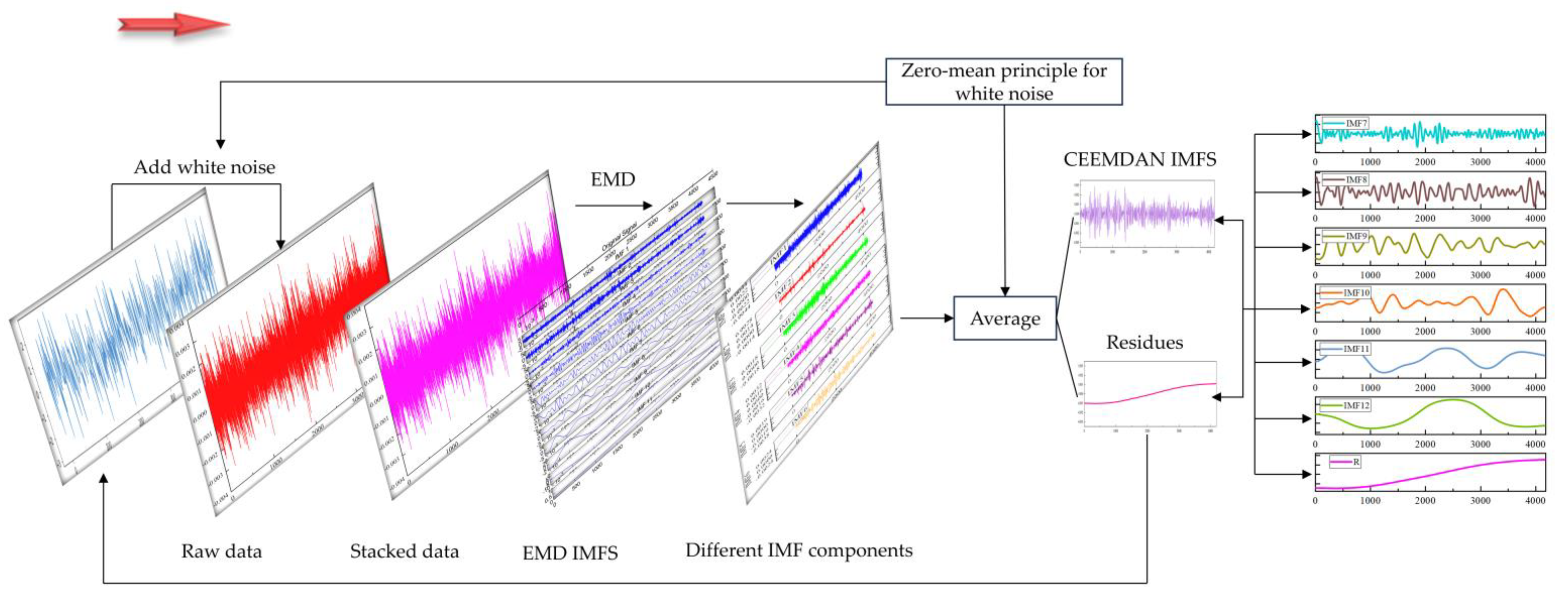
2.1. CEEMDAN

EMD algorithm is an adaptive method used for analyzing nonlinear signals. This method can decompose complex time series into multiple Intrinsic Mode Functions (IMFs) and residue signals (R) with different frequencies and scales. However, the biggest drawback of EMD is the occurrence of endpoint effects and mode-mixing phenomena when used. To address the mode mixing issue in EMD, the EEMD algorithm proposes a noise-assisted data analysis method to overcome the deficiencies of the EMD method. At each step of signal decomposition, white noise with zero means, and fixed variance is added to the signal being decomposed, effectively resolving the endpoint effects and mode-mixing phenomena encountered by the EMD algorithm. However, this method still has a drawback: it cannot eliminate the added white noise, thereby affecting the extraction of feature information.

Therefore, based on EEMD, the CEEMDAN algorithm is proposed by adaptively introducing white noise and performing cumulative averaging after obtaining the IMF components to improve EEMD. This method effectively addresses the modal aliasing phenomenon in EMD and overcomes the issues of incompleteness and large reconstruction errors in EEMD [43]. Figure 1 briefly describes the CEEMDAN process.

The steps of this decomposition method can be represented by Equations (1)–(9):

Step 1: In the original displacement signal $X\left(t\right)$, white noise ${\omega }^e\left(t\right)$ is added, represented mathematically as:

$$X^e\left(t\right)=X\left(t\right)+{\xi }_0{\omega }^e\left(t\right), e=1,2,3,\dots ,E$$

(1)

where ${\xi }_0$ is the noise factor; ${\omega }^e\left(t\right)$ is the white noise added for the $e$th time; $E$ is the number of integration times, which is usually set to 15~25; $X^e\left(t\right)$ is the signal after adding white noise for the $e$th time.

Step 2: The first IMF component ${\overline{IMF}}_1\left(t\right)$ is obtained by performing EMD decomposition on $X^e\left(t\right)$ and then taking the average value, that is:

$${\overline{IMF}}_1\left(t\right)={\displaystyle \frac{1}{E}}{\displaystyle \sum _{i=1}^{M}IM{F}_1^e\left(t\right)}$$

(2)

$$r_1\left(t\right)=X\left(t\right)-{\overline{IMF}}_1\left(t\right)$$

(3)

where ${\overline{IMF}}_1\left(t\right)$ is the first IMF component after EMD decomposition of the signal and $r_1\left(t\right)$ is the first residual signal.

Step 3: The signal $r_1\left(t\right)+{\xi }_{1}EM{D}_1\left({\omega }^e\left(t\right)\right)$ is decomposed using EMD to obtain the second IMF component and the residue signal as shown below:

$${\overline{IMF}}_2\left(t\right)={\displaystyle \frac{1}{E}}{\displaystyle \sum _{e=1}^{E}EM{D}_1\left(r_1\left(t\right)+{\xi }_{1}EM{D}_1\left({\omega }^e\left(t\right)\right)\right)}$$

(4)

$$r_2\left(t\right)=r_1\left(t\right)-{\overline{IMF}}_2\left(t\right)$$

(5)

where ${\xi }_1$ is the first noise factor, ${\omega }^e\left(t\right)$ is the white noise added for the $e$th time,$EM{D}_1\left(\cdot \right)$ represents the first IMF obtained by EMD, ${\overline{IMF}}_2\left(t\right)$ is the second IMF component after EMD decomposition of the signal and $r_2\left(t\right)$ is the second residual signal.

Step 4: Repeat steps (2) and (3) to obtain residuals and IMF components, that is:

$$r_k\left(t\right)=r_{k-1}\left(t\right)-{\overline{IMF}}_k\left(t\right), k=2,3,\dots ,K$$

(6)

$${\overline{IMF}}_{k+1}\left(t\right)={\displaystyle \frac{1}{E}}{\displaystyle \sum _{i=1}^{E}EM{D}_1\left(r_k\left(t\right)+{\xi }_{k}EM{D}_k\left({\omega }^i\left(t\right)\right)\right)}$$

(7)

where $EM{D}_k\left(\cdot \right)$ denotes the $k$th IMF component obtained by EMD and $K$is the total number of modes.

Step 5: Repeat step (4), and when the signal no longer exceeds two extreme points during decomposition, indicating that the residual signal cannot be further decomposed, the algorithm stops. The residual signal can be represented as:

$$R\left(t\right)=X\left(t\right)-{\displaystyle \sum _{k=1}^{K}IM{F}_k\left(t\right)}$$

(8)

After undergoing CEEMDAN decomposition, the original displacement sequence is iteratively decomposed into $n$IMF components, denoted as ${\overline{IMF}}_i\left(t\right)$, $i=1,2,3,\dots ,n$. Finally, the displacement sequence $X\left(t\right)$ after CEEMDAN decomposition can be represented as:

$$X\left(t\right)={\displaystyle \sum _{k=1}^K\overline{IM{F}_k}\left(t\right)}+R\left(t\right)$$

(9)

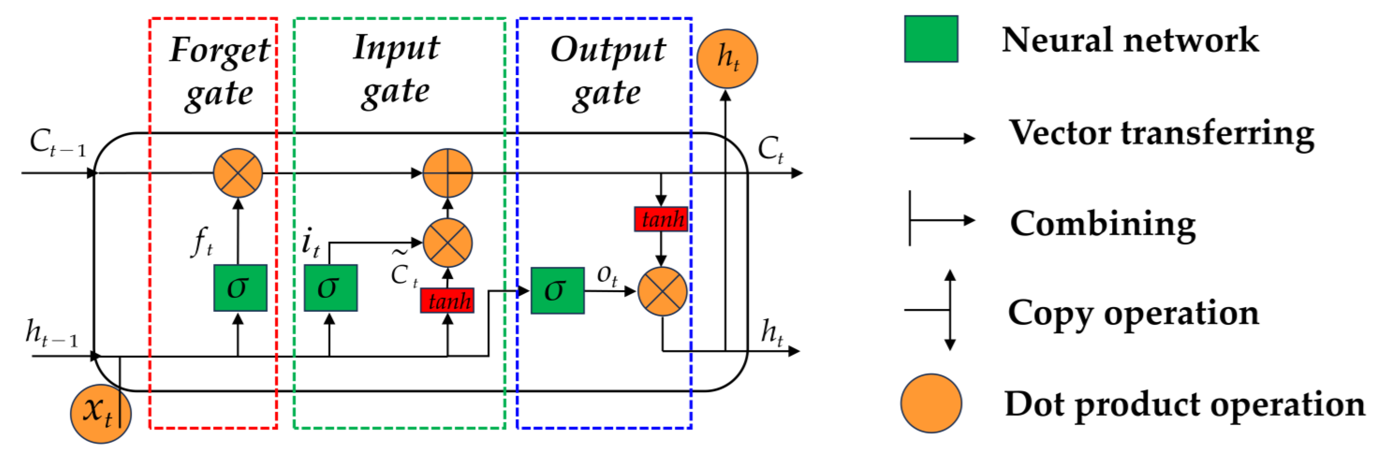
2.2. LSTM Networks

Recurrent Neural Networks (RNNs) are specialized networks designed for handling sequential data [44]. As illustrated in Figure 2, an RNN contains an internal loop structure, enabling the propagation of previous time-step state information to the current state to establish temporal relationships and exhibit dynamic behavior [45]. The output at the time step $t$ is determined by the input at the time step $t$ and the output at the time step $t-1$. However, as time progresses, information loss occurs during the propagation process, leading to issues such as gradient vanishing in RNNs, thereby diminishing their ability to handle long-term dependencies in time series data [46]. The computational process of RNNs can be represented by Equations (10) and (11):

$$h_t=tanh\left(U{x}_t+W{h}_{t-1}+b_h\right)$$

(10)

$$y_t=soft\max \left(V{h}_t+b_y\right)$$

(11)

where $x_t$, $h_t$ and $y_t$ denote the input vectors, hidden unit states, and outputs at moment $t$, respectively, and $W$, $U$ and $V$ denote the weight matrices of the corresponding RNN layers. The parameters $b_h$ and $b_y$ are bias vectors.

In response to the problem of gradient vanishing and other issues commonly encountered in RNNs, Hochreiter et al. proposed LSTM to address this challenge. LSTM, based on the original network architecture, replaces the RNN units in the hidden layers with LSTM units and resets the computational nodes. A basic LSTM neural unit is controlled by three gates: the input gate, the output gate, and the forget gate. Its structure is illustrated in Figure 3.

In Figure 3, $x_t$ is the input at the current moment, $h_t$ and $h_{t-1}$ represent the state of the hidden layer at the current moment and the previous moment, respectively; $C_t$ and $C_{t-1}$ represent the state of the cell at the current moment and the previous moment, respectively, $x_t$, $h_t$, $C_t$ are fed into the LSTM through these three gate structures. each gate computes the input information and decides whether to activate it or not according to its logical function. In this case, the forgetting gate $f_t$ discards the information that is considered unimportant by the memory cell, the input gate $i$ recognizes the new information that needs to be retained in the cell state and updates it with the activation function, and the output gate $o_t$ decides the output based on the cell state. The above process can be expressed by Equations (12)–(16):

$$i_t=\sigma \left(T_i{x}_t+V_i{h}_{t-1}+q_i\right)$$

(12)

$$f_t=\sigma \left(T_f{x}_t+V_f{h}_{t-1}+q_f\right)$$

(13)

$$C_t=f_t\otimes C_{t-1}+i_t\otimes tanh\left(T_C{x}_t+V_C{h}_{t-1}+q_C\right)$$

(14)

$$o_t=\sigma \left(T_o{x}_t+V_o{h}_{t-1}+q_o\right)$$

(15)

$$h_t=o_t\otimes tanh\left(C_t\right)$$

(16)

where $\sigma$ and $tanh$ respectively denote the Sigmoid activation function and the hyperbolic tangent activation function, $T$ and $V$ denote the parameter matrices, $q$ denotes the bias vector, and $\otimes$ denotes element-wise multiplication.

2.3. Clustering Methods

After decomposing the signals using the CEEMDAN algorithm, the power spectral density (PSD) of each IMF is computed to identify the energy distribution characteristics of each signal across different frequency bands and their differences. The formula for calculating the power spectral density can be presented by Equations (17)–(19):

The Fourier transform of the deformation time series $x\left(t\right)$ can be represented as:

$$X\left(f,T_r\right)={\displaystyle {\int }_0^{T_r}x\left(t\right)e^{-i2\pi ft}}dt$$

(17)

where: $f$ is the frequency, and $T_r$ is the length of the deformation sequence. For a certain discrete frequency, it is represented as $f_n$.

$$X_n={\displaystyle \frac{X\left(f_n,T_r\right)}{\Delta t}}$$

(18)

where: $f_n=n/\left(N\Delta t\right)$, $n=1,2,\dots ,N$, represents the time interval, $\Delta t$ represents the number of sampling points, $N=T_r/\Delta t$. Then the power spectral density can be represented as:

$$P_n={\displaystyle \frac{2\Delta t}{N}}{\left|X_n\right|}^2$$

(19)

Subsequently, IMF signals are clustered based on their energy distribution characteristics within different frequency ranges, along with their frequency peak characteristics. If the energy distribution and signal peak characteristics are similar, the IMF signals are grouped into similarity clusters; otherwise, no clustering is done. Finally, the clustered signals are combined to form a few reconstructed sub-signals of the original time series signal.

2.4. Framework of the CEEMDAN-SC-LSTM Prediction Method

The structure of the proposed CEEMDAN-SC-LSTM prediction model is illustrated in Figure 4. The specific steps are as follows:

Step 1: Use the CEEMDAN algorithm to decompose the monitoring data into a series of IMF components and a residual term.

Step 2: Perform spectral analysis on each decomposed modal component. Cluster and aggregate the IMF components with similar frequency domain characteristics, reconstructing them into structural response signals of different scales and amplitudes.

Step 3: The reconstructed sub-signals were divided into a predetermined proportion of training and testing sets. These sets were then fed into the trained LSTM model for prediction.

Step 4: The predicted results were combined to form the final prediction outcome.

2.5. Evaluation Metrics

In terms of model evaluation, the selected evaluation metrics in this study include RMSE, Mean Absolute Error (MAE), and Mean Absolute Percentage Error (MAPE), which are used to assess the predictive performance of the proposed model. These metrics can be mathematically represented by Equations (20)–(22):

(1) RMSE. The smaller the RMSE value, the smaller the difference between the model’s predicted values and the actual values, indicating higher prediction accuracy of the model. The RMSE equation is:

$$\mathrm{RMSE}\left(y,\widehat{y}\right)=\sqrt{{\displaystyle \frac{1}{n}}{\displaystyle \sum _1^n{\left(y_i-{\widehat{y}}_i\right)}^2}}$$

(20)

(2) MAE. MAE represents the average of the absolute differences between the predicted values and the actual values, meaning that a smaller MAE value indicates a smaller prediction error and higher prediction accuracy of the model. The MAE equation is:

$$\mathrm{MAE}\left(y,\widehat{y}\right)={\displaystyle \frac{1}{n}}{\displaystyle \sum _1^n\left|y_i-{\widehat{y}}_i\right|}$$

(21)

(3) MAPE. In the MAPE evaluation criteria, the smaller the value of MAPE, the smaller the difference between the predicted and true values of the model, and the higher the predictive accuracy of the model. The MAPE equation is:

$$\mathrm{MAPE}\left(y,\widehat{y}\right)={\displaystyle \frac{100\%}{n}}{\displaystyle \sum _{i=1}^n\frac{\left|y_i-{\widehat{y}}_i\right|}{max\left(ϵ,\left|y_i\right|\right)}}$$

(22)

where ${\widehat{y}}_i$ is the predicted value, $y_i$ is the original true value, $n$ is the total number of predicted values, and $ϵ$ is an arbitrarily small but strictly positive number in the MAPE formula to avoid uncertain results at zero.

3. Experimental Validation and Analysis

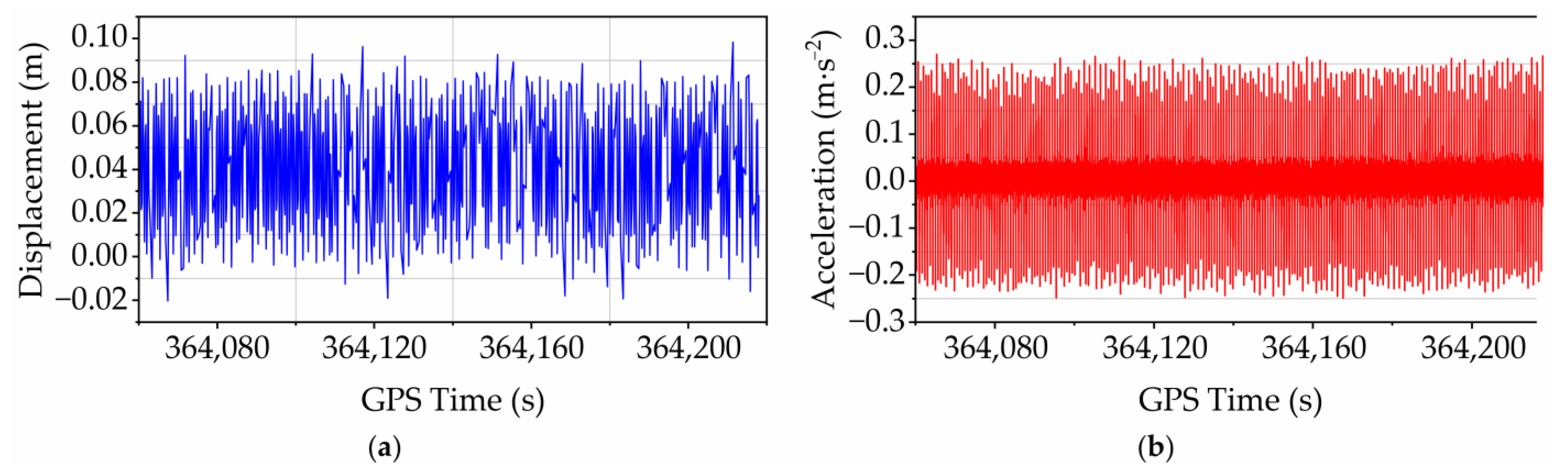
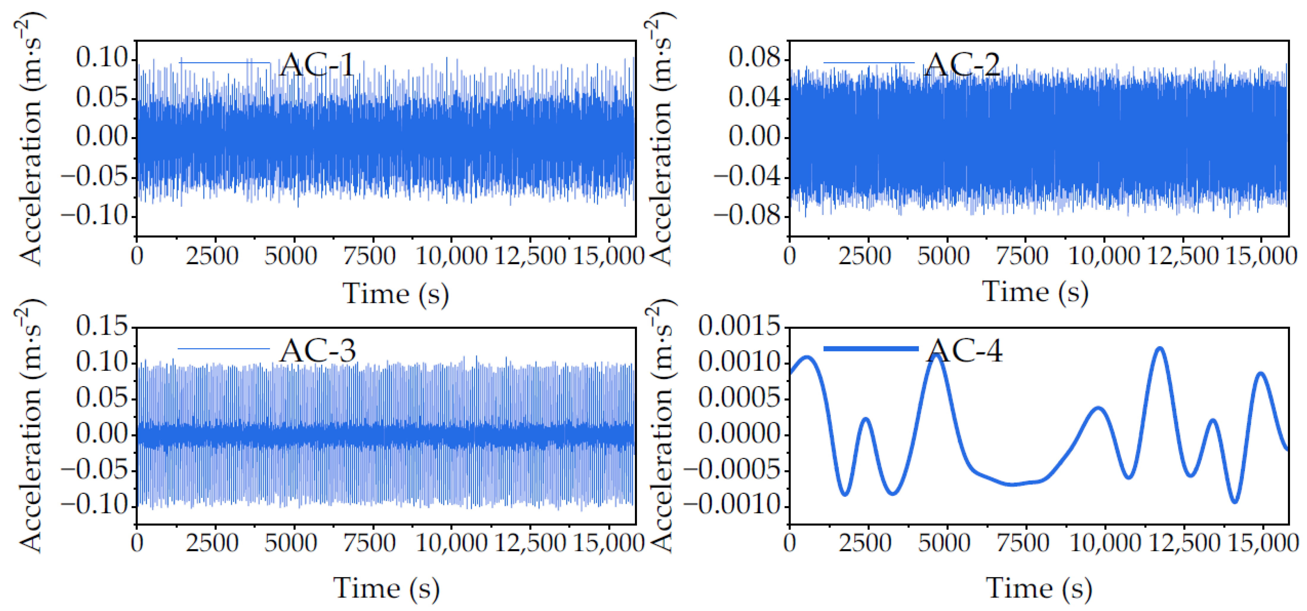
3.1. The Experiment of Shaking Table

To validate the predictive performance of the proposed prediction model, deformation simulation experiments were conducted using a shake table at Beijing University of Civil Engineering and Architecture in March 2024. The experiment employed an IPMV GNSS/accelerometer integrated receiver, with a GNSS sampling rate of 5 Hz and an accelerometer sampling rate of 100 Hz. A calibration method was used to align the accelerometer axis with the X-axis of the vibration table. The specific structure of the vibration platform and the installation position of the measurement simulation deformation sensor are shown in Figure 5. Additionally, a control platform was used to set the sampling rate and vibration amplitude.

The raw acceleration data generated by the vibration is depicted in Figure 6, illustrating the system’s capability to accurately capture crucial moments of instantaneous acceleration increase. The graph distinctly shows the instances of acceleration spikes throughout the experiment. This graphical representation underscores the precision and effectiveness of the monitoring system in capturing dynamic changes in acceleration.

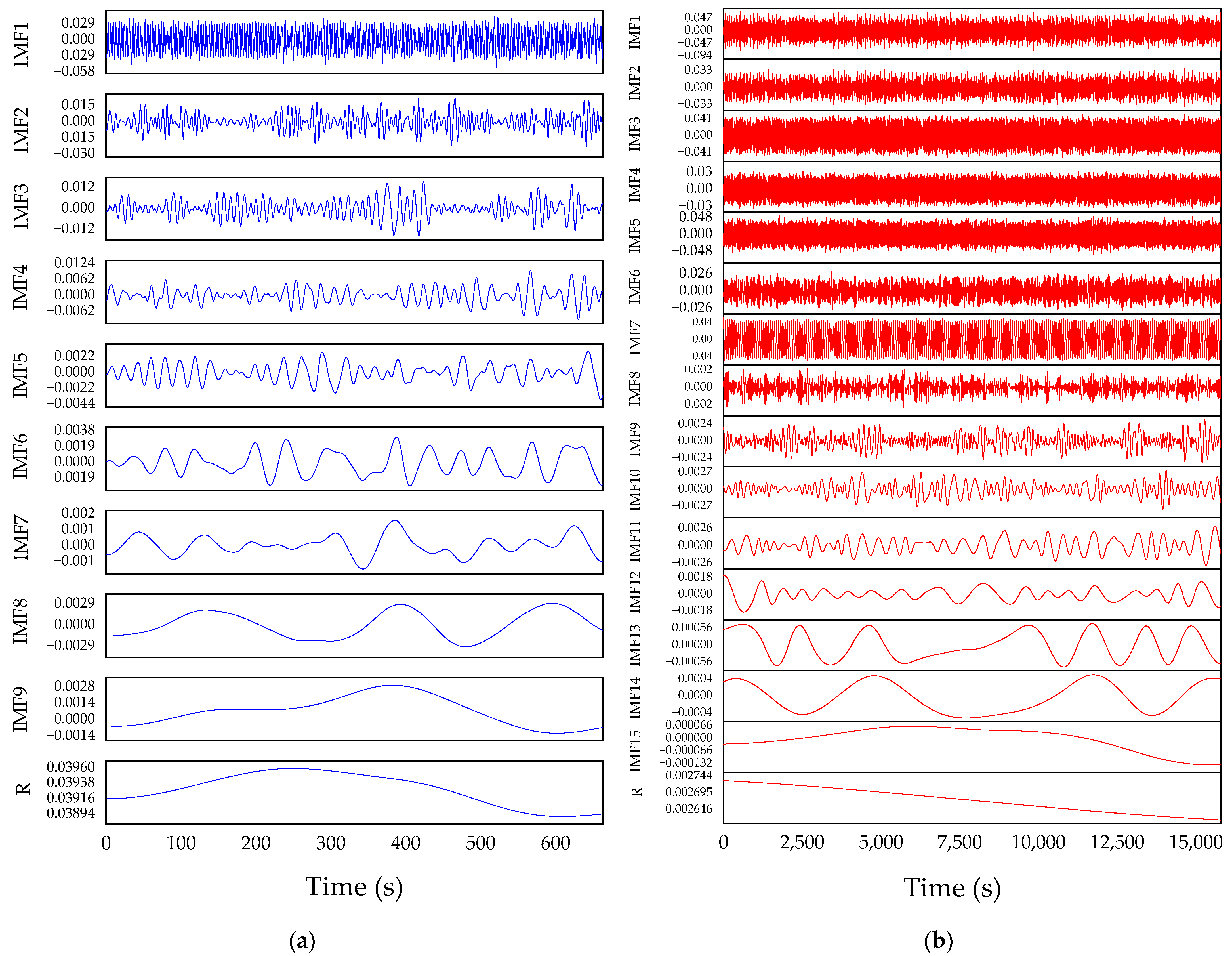
3.2. CEEMDAN Decomposition

GNSS data and acceleration data generated under the conditions of a frequency of 2 Hz and an amplitude of 30 mm (displacement) were selected as the research data for this study. The observation period spans from GPS time 364,060 s to 364,218 s. Figure 7 shows the distribution of displacement and acceleration after processing the original data within the specified time range.

The GNSS displacement and acceleration data generated by the vibration were decomposed using CEEMDAN, yielding the decomposition results shown in Figure 8. The displacement sequence was decomposed into nine IMF sequences ranging from high to low frequency, along with a residual component. Similarly, the acceleration data were decomposed into fifteen IMF components and their corresponding residuals. After decomposition, the high-frequency vibration information of the displacement data was mainly concentrated in IMF1, exhibiting relatively large amplitudes. As for the acceleration data, high-frequency information was primarily distributed across IMF1 to IMF7, typically containing noise and rapid variations in the signal, which could reflect the transient response characteristics of the vibration system.

3.3. Similarity Clustering

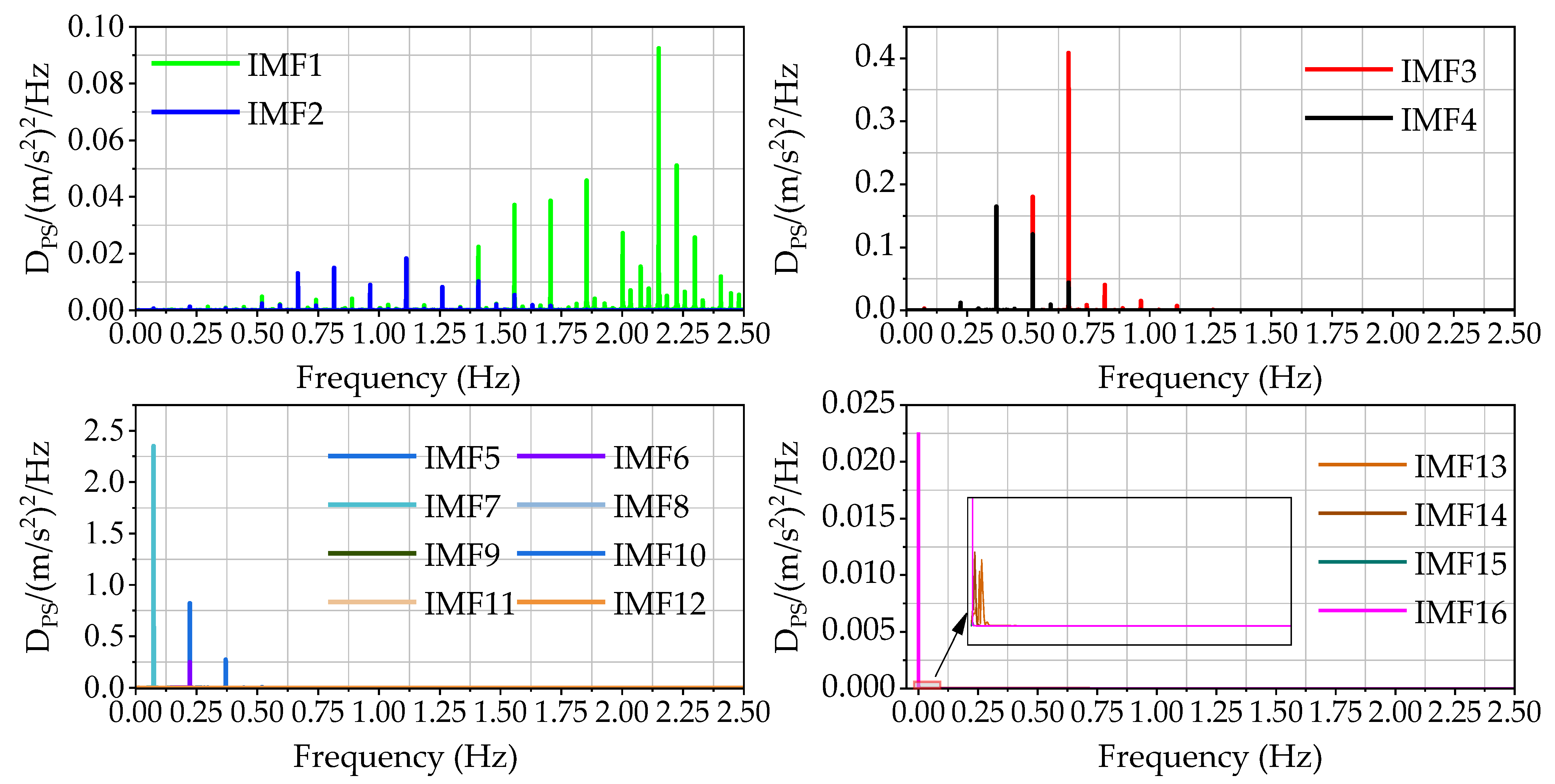
3.3.1. Spectrum Analysis

After decomposing the GNSS displacement and acceleration sequences using CEEMDAN, a series of IMF sequences were generated, and frequency domain features were extracted from these sequences. Building upon time domain analysis, clustering based on the frequency domain similarity of the sub-sequences was conducted. Through spectral analysis, the main frequencies of each sub-sequence were determined.

For the displacement sequence, as the order of IMF increased, the energy distribution decreased from high to low frequencies. As shown in Figure 9, the energy of IMF1 was mainly concentrated in the range of 1 Hz to 1.5 Hz; IMF2 to IMF3 exhibited energy distribution primarily in the range of 0.5 Hz to 1 Hz; IMF4 to IMF7 had energy concentrated near 0.25 Hz, while IMF8 and other components were mainly centered around 0 Hz. Based on these energy distribution characteristics, IMF sub-sequences with concentrated energy distributions were categorized into different groups according to their dominant frequency features.

As shown in Figure 10, for the acceleration time series, the energy distribution of its IMF sequences also exhibited a similar trend, albeit with different frequency ranges. The energy distribution of IMF1 and IMF2 was primarily concentrated in the range of 1 Hz to 2.25 Hz; IMF3 and IMF4 showed energy distribution mainly in the range of 0.25 Hz to 0.75 Hz; IMF5 to IMF12 had energy concentrated in the range of 0 Hz to 0.25 Hz, while IMF13 and other components were likewise mainly centered around 0 Hz. Similarly, based on these energy distribution characteristics, the IMF sequences with concentrated energy distributions were categorized into different groups according to their dominant frequency features.

3.3.2. Reconstruction by Superposition

The clustered results of displacement and acceleration subsequences were reconstructed by superposition. As shown in Figure 11 and Figure 12, In the displacement sequence, IMF1 is separately considered as a sequence, forming the reconstructed sequence GS-1; IMF2 and IMF3 are superimposed to form the reconstructed sequence GS-2; IMF4 to IMF7 are superimposed to form the reconstructed sequence GS-3; while the remaining components such as IMF8 are superimposed to form the reconstructed sequence GS-4.

Similarly, in the acceleration sequence, IMF1 and IMF2 are superimposed to form the reconstructed sequence AC-1; IMF3 and IMF4 are superimposed to form the reconstructed sequence AC-2; IMF5 to IMF12 are superimposed to form the reconstructed sequence AC-3; IMF13 and the remaining components are superimposed to form the reconstructed sequence AC-4. These reconstructed sequence signals not only retain the basic information of the original sequence but also possess different time scales and amplitudes, which are not present in the original sequence. Based on these reconstructed signals, they serve as inputs for subsequent deep learning of time series data, to further explore and analyze the potential information and patterns in these sequences.

3.4. Training of LSTM Model and Prediction Results

3.4.1. Experimental Settings

In this study, the experiments were implemented in Python 3.7 on a PC with AMD Ryzen 9 5900HX with Radeon Graphics 3.30 GHz and NVIDIA GeForce RTX 3050 Ti Laptop GPU, with a memory size of 16.00 GB. The clustering algorithm and the CEEMDAN algorithm were implemented in MATLAB 2022b.

For the LSTM prediction task targeting GNSS displacement and acceleration data, we divided the dataset into 70% for training, 15% for testing, and 15% for validation to ensure effective training and objective evaluation of the model. After normalizing the training set, it was input into the model for training. The Adam [47] optimization algorithm was employed, and through iterative exploration of various parameter combinations, the optimal hyperparameters were determined based on performance on the validation dataset. For GNSS displacement prediction, the final selected parameters are as follows: an initial learning rate of 0.001, 1 layer in the network, 370 hidden units, a dropout probability of 0.5, and decay rates of 0.99 for the first order and 0.999 for the second order. For acceleration prediction, the final selected parameters are as follows: an initial learning rate of 0.005, 2 layers in the network, 490 hidden units, a dropout probability of 0.5, and decay rates of 0.99 for the first order and 0.999 for the second order. To prevent overfitting during the training of the LSTM model, the learning rate was reduced to one-tenth of its initial value after 250 iterations.

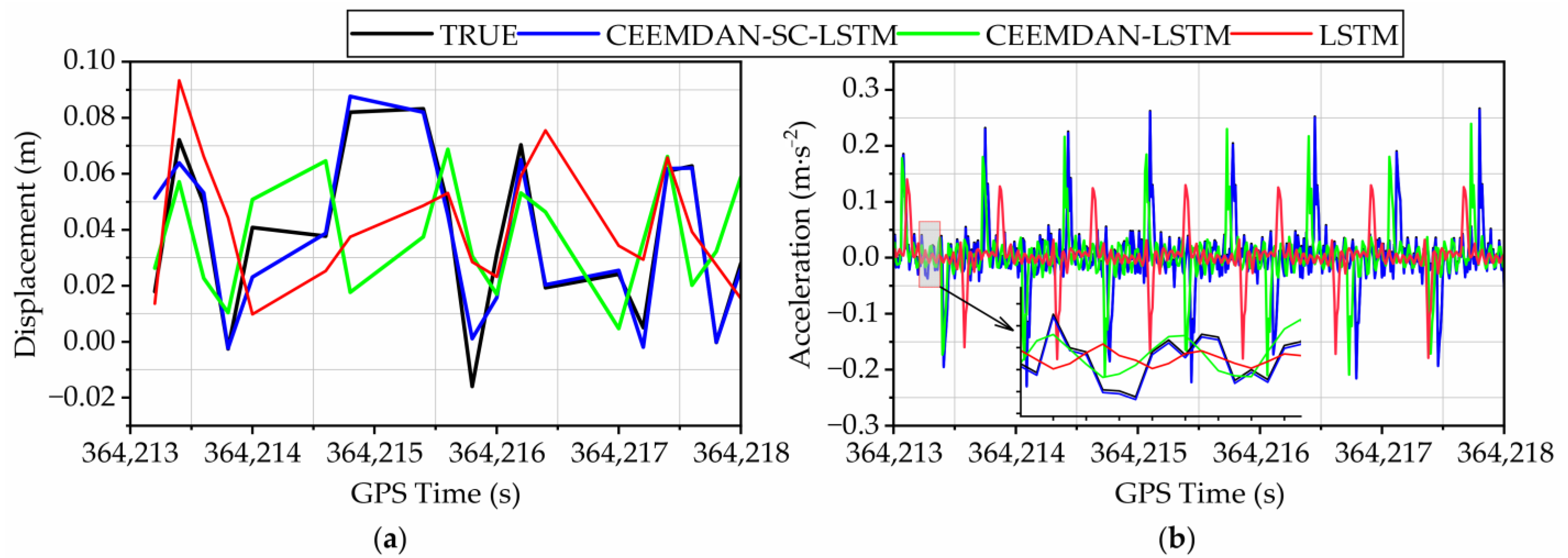
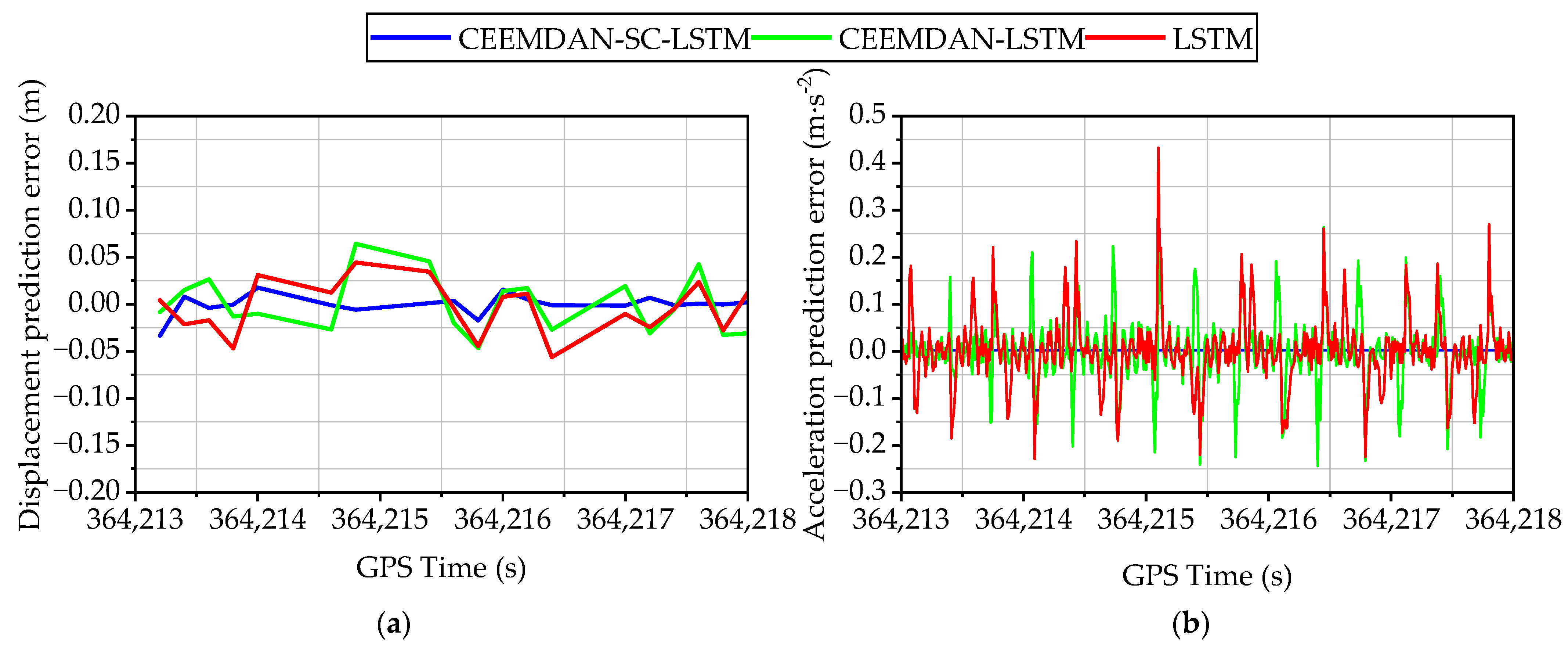
3.4.2. Analysis of Predicted Results

To further evaluate the advantages of the CEEMDAN-SC-LSTM model in deformation prediction, this study selected the CEEMDAN-LSTM and a single LSTM prediction model as comparative experiments. To visually compare the predictive performance of different models, a comparison chart of the prediction results, as shown in Figure 13, was plotted. Additionally, to further illustrate the prediction accuracy of the three models, their prediction errors were visualized in Figure 14.

Figure 13 and Figure 14 depict the prediction and error curves for GNSS displacement and acceleration, respectively, obtained by the CEEMDAN-SC-LSTM, CEEMDAN-LSTM, and LSTM models. It is evident from the figures that compared to CEEMDAN-LSTM and LSTM, the CEEMDAN-SC-LSTM prediction model exhibits closer alignment with the real values and smaller prediction errors for both GNSS displacement and acceleration. These findings indicate that the proposed model can more accurately capture the dynamic variations in the data, thereby generating more precise predictions.

Furthermore, by comparing the prediction error metrics of the three different models, we can further validate the high-precision predictive capability of the proposed model. As shown in

Table 1. Compares the predictive performance of the three models.

Model	RMSE		MAE		MAPE%
	Displacement/m	Acceleration/m/s2	Displacement/m	Acceleration/m/s2	Displacement	Acceleration
CEEMDAN-SC-LSTM	0.011	0.002	0.007	0.002	0.346	0.516
CEEMDAN-LSTM	0.030	0.068	0.026	0.046	7.220	4.577
LSTM	0.028	0.070	0.023	0.045	6.879	5.550

, for both GNSS displacement and acceleration predictions, the CEEMDAN-SC-LSTM model achieves the minimum values in terms of RMSE, MAE, and MAPE. Specifically, in GNSS displacement prediction, the CEEMDAN-SC-LSTM model’s RMSE value is 0.0107 m, significantly lower than that of the CEEMDAN-LSTM model (0.0301 m) and the LSTM model (0.0278 m). Similarly, in acceleration prediction, the RMSE value of the proposed model is also substantially lower than the other two models. Additionally, the proposed model demonstrates significant advantages in terms of MAE and MAPE metrics. These results demonstrate that the proposed model exhibits higher predictive accuracy and stronger generalization ability in predicting GNSS displacement and acceleration.

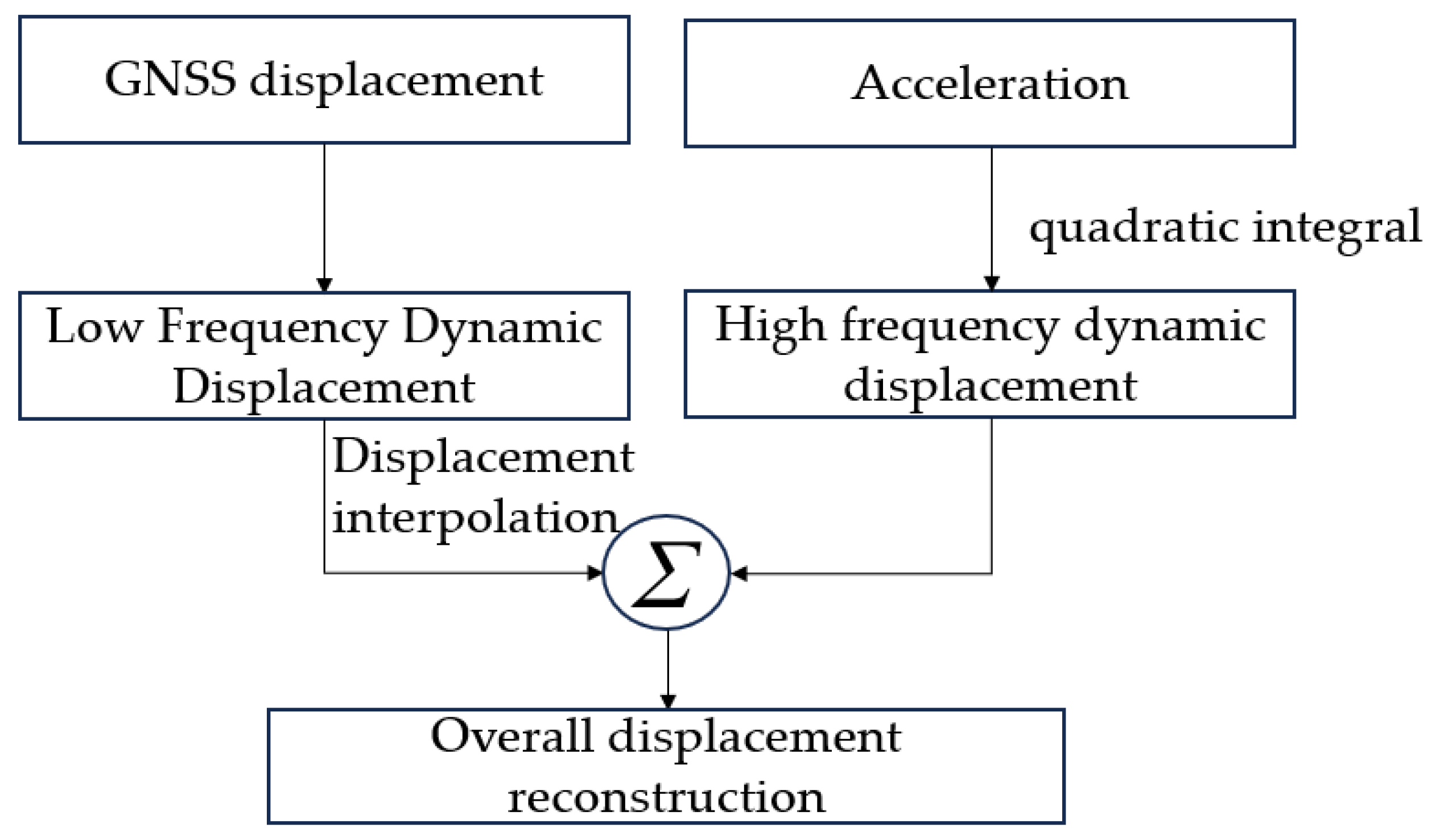
3.5. Reconstruction of Overall Deformation by Prediction Results

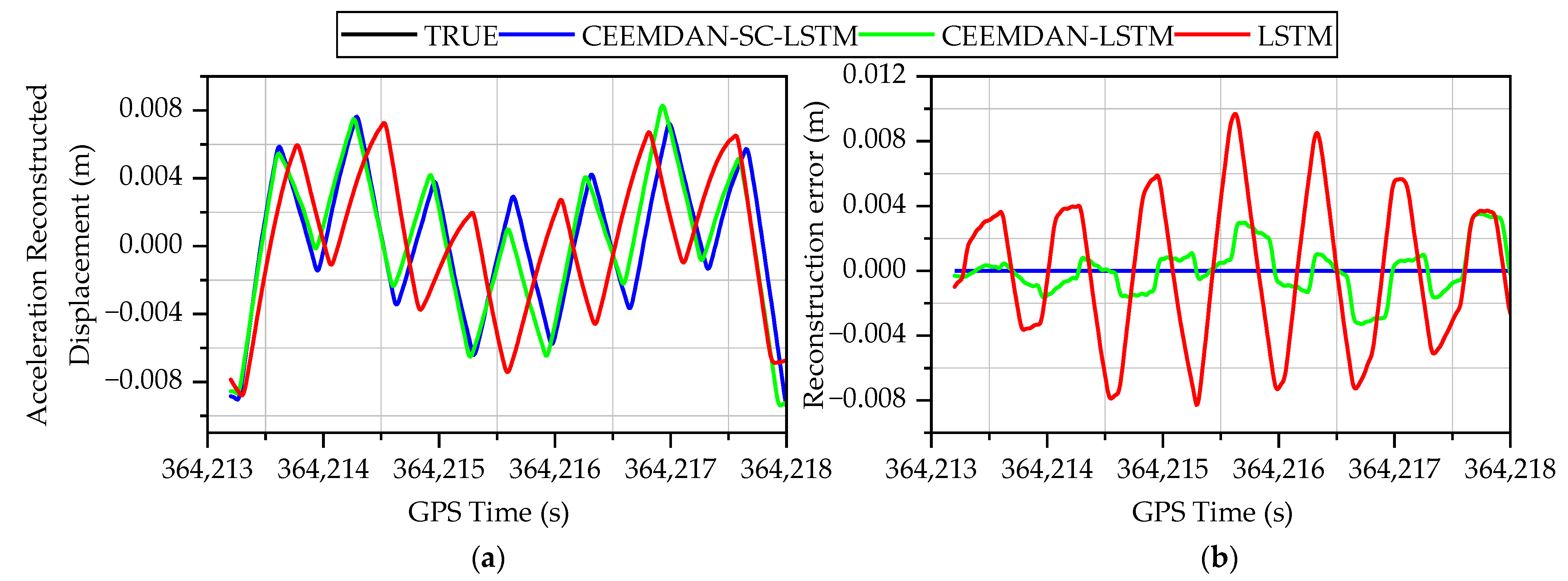
Acceleration Reconstructed Displacement

The dynamic displacement reconstruction based on the acceleration predictions from the CEEMDAN-SC-LSTM, CEEMDAN-LSTM, and LSTM models is shown in Figure 15, along with the reconstruction errors. To evaluate the reconstruction accuracy, the mean peak error ($\overline{E}$), correlation coefficient (R), and RMSE were used as metrics, with the statistical results presented in

Table 2. Statistics of Reconstructed Displacement Errors from Predicted Acceleration.

Method	Model	$\overline{\mathit{E}}$	R	RMSE/m
Acceleration Reconstructed Displacement	CEEMDAN-SC-LSTM	0.007	0.999	0.003
	CEEMDAN-LSTM	0.011	0.939	0.015
	LSTM	0.037	0.454	0.044

.

Figure 15 provides a visual comparison of the performance of the CEEMDAN-SC-LSTM, CEEMDAN-LSTM, and LSTM models in reconstructing displacement from predicted acceleration. It is evident that the displacement curve reconstructed using the CEEMDAN-SC-LSTM model aligns most closely with the true values, almost perfectly overlapping, whereas the other two models exhibit noticeable deviations. As shown in Table 2, the correlation coefficient between the reconstructed displacement from the CEEMDAN-SC-LSTM model and the true values is as high as 99%, with an RMSE of 3 mm and an average peak error of less than 0.01. These experimental results indicate that the CEEMDAN-SC-LSTM model achieves high accuracy in displacement reconstruction from predicted acceleration data.

3.6. Overall Deformation Reconstruction

3.6.1. True Deformation Sequence

Figure 16 illustrates the specific implementation process of overall dynamic deformation reconstruction. This involves removing high-frequency noise from acceleration data, performing a frequency-domain second integral to remove linear trend terms, and obtaining high-frequency dynamic displacements. The GNSS displacement series retains low-frequency displacements and is interpolated to match the sampling rate of the high-frequency dynamic displacement signals reconstructed from the acceleration data. Finally, the high-frequency dynamic displacements reconstructed from the acceleration data and the low-frequency dynamic displacements extracted from the GNSS data are combined to reconstruct the overall structural deformation.

To extract low-frequency dynamic displacement information, the displacement data was filtered. Next, the acceleration data was denoised and detrended to obtain high-frequency dynamic displacements after the second integral. Through displacement interpolation, the displacement data collected by the two sensors was used for overall deformation reconstruction, resulting in the overall displacement shown on the left side of Figure 17. The right side of Figure 17 displays the deformation reconstruction sequences for the selected time period in this study, which will serve as the basis for subsequent analyses.

3.6.2. Reconstruction of Overall Deformation Using Predicted Values

Figure 18 shows the overall deformation reconstruction based on GNSS displacements and accelerations predicted by the CEEMDAN-SC-LSTM model.

Table 3. Statistics of Reconstructed Displacement Errors from Predicted Acceleration.

Method	Model	$\overline{\mathit{E}}$	R	RMSE/m
Overall Displacement Reconstruction	CEEMDAN-SC-LSTM	0.004	0.958	0.005
	CEEMDAN-LSTM	0.018	0.281	0.020
	LSTM	0.016	0.272	0.019

provides detailed error statistics for the overall deformation reconstruction. As shown in the table, the correlation coefficient between the displacements reconstructed by the CEEMDAN-SC-LSTM model and the reference values is 96%, with an RMSE of 0.005 m and a mean peak error of 0.004. Compared to the CEEMDAN-LSTM and LSTM prediction models, the CEEMDAN-SC-LSTM model performs best in overall dynamic displacement reconstruction, closely matching the true values and accurately capturing the deformation trends and details. In summary, the CEEMDAN-SC-LSTM model excels in the overall deformation reconstruction after prediction, offering higher accuracy and reliability.

4. Conclusions

Deformation prediction is essential for the healthy operation of large structural buildings. This study investigates a similarity clustering deformation prediction method based on GNSS/accelerometer time-frequency analysis, achieving overall deformation reconstruction through displacement and acceleration predictions. The following conclusions are drawn from the analysis of deformation monitoring data simulated by a shaking table experiment.

(1)

The monitoring sequences are decomposed into several simple signal components for each monitoring data by the CEEMDAN algorithm, which effectively reduces the adverse effects of the nonlinear and nonstationary characteristics of the monitoring sequences on the subsequent model training.

(2)

A data response reconstruction is proposed by analyzing time-frequency feature similarity and clustering. The clustered monitoring sequences exhibit complex and distinct characteristics, allowing better capture of key features in the structural deformation process. Shaking table experiment results showed that the proposed deformation prediction framework could offer an average prediction error of RMSE = 0.011 m for predicted GNSS displacement and RMSE = 0.002 m/s^2 for predicted acceleration. When compared to the CEEMDAN-LSTM and LSTM prediction models, the proposed model exhibits higher prediction accuracy and reliability.

(3)

The overall displacement reconstructed by the method proposed in this paper has a strong correlation with the reference displacement, The experimental results show that the RMSE of the displacement reconstructed from predicted acceleration is less than 1 mm, with a reconstruction similarity of over 99%. Furthermore, the overall displacement reconstruction similarity can reach over 95%. The GNSS/accelerometer integrated displacement reconstruction algorithm accurately identifies structural deformation, thereby enhancing the precision and reliability of deformation monitoring. This algorithm can be applied to health monitoring and early warning systems for large structures.

In summary, the predictive model proposed in this paper demonstrates significant advantages in predictive performance, providing valuable insights for structural deformation prediction. However, when making predictions, we must pay close attention to the choice of input layer indicator variables, relevant parameters, and network architecture. A reasonable combination of these elements is crucial for enhancing prediction stability and accuracy, while also effectively reducing network training time. This necessitates thorough parameter tuning and network structure design during model construction and training to ensure the model can fully capture the key information in the data and accurately predict structural deformations. It is also important to note that structural deformation results from the interplay of various factors, including but not limited to material properties and external environments. Therefore, we should comprehensively consider these influencing factors when training the network. Future research can further explore how to integrate more physical knowledge and engineering experience to optimize model design, as well as leverage advanced computational techniques and algorithms to improve training efficiency and predictive accuracy.

References

- Han, H.; Ma, W.; Xu, Q.; Li, R.; Xu, T. A Welch-Ewt-Svd Time–Frequency Feature Extraction Model for Deformation Monitoring Data. Measurement 2023, 222, 113709. [Google Scholar] [CrossRef]
- Xiong, C.; Niu, Y. Investigation of the Dynamic Behavior of a Super High-Rise Structure Using Rtk-Gnss Technique. KSCE J. Civ. Eng. 2019, 23, 654–665. [Google Scholar] [CrossRef]
- Li, H.; Xu, Q.; He, Y.; Fan, X.; Yang, H.; Li, S. Temporal Detection of Sharp Landslide Deformation with Ensemble-Based Lstm-Rnns and Hurst Exponent. Geomat. Nat. Hazards Risk 2021, 12, 3089–3113. [Google Scholar] [CrossRef]
- Shen, W.; Zhi, J.; Wang, Y.; Sun, J.; Lin, Y.; Li, Y.; Jiang, W. Two-Step Cfar-Based 3d Point Cloud Extraction Method for Circular Scanning Ground-Based Synthetic Aperture Radar. Appl. Sci. 2023, 13, 7164. [Google Scholar] [CrossRef]
- Yi, Z.; Kuang, C.; Wang, Y.; Yu, W.; Cai, C.; Dai, W. Combination of High- and Low-Rate Gps Receivers for Monitoring Wind-Induced Response of Tall Buildings. Sensors 2018, 18, 4100. [Google Scholar] [CrossRef] [PubMed]
- Lorenz, R.; Petryna, Y.; Lubitz, C.; Lang, O.; Wegener, V. Thermal Deformation Monitoring of a Highway Bridge: Combined Analysis of Geodetic and Satellite-Based Insar Measurements with Structural Simulations. J. Civ. Struct. Health Monit. 2024, 14, 1237–1255. [Google Scholar] [CrossRef]
- Ogaja, C.; Wang, J.; Rizos, C. Detection of Wind-Induced Response by Wavelet Transformed Gps Solutions. J. Surv. Eng. 2003, 129, 99–104. [Google Scholar] [CrossRef]
- Jing, C.; Huang, G.; Zhang, Q.; Li, X.; Bai, Z.; Du, Y. Gnss/Accelerometer Adaptive Coupled Landslide Deformation Monitoring Technology. Remote Sens. 2022, 14, 3537. [Google Scholar] [CrossRef]
- Han, H.; Wang, J.; Meng, X. Reconstruction of Bridge Dynamics Usingintegrated Gps and Accelerometer. Zhongguo Kuangye Daxue Xuebao/J. China Univ. Min. Technol. 2015, 44, 549–556. [Google Scholar]
- Yu, J.; Meng, X.; Yan, B.; Xu, B.; Fan, Q.; Xie, Y. Global Navigation Satellite System-Based Positioning Technology for Structural Health Monitoring: A Review. Struct Control Health Monit. 2020, 27, e2467. [Google Scholar] [CrossRef]
- Qi, X.; Hong, C.; Ye, T.; Gu, L.; Wu, W. Frequency Reconstruction Oriented Emd-Lstm-Am Based Surface Temperature Prediction for Lithium-Ion Battery. J. Energy Storage 2024, 84, 111001. [Google Scholar] [CrossRef]
- Yan, Y.; Wang, X.; Ren, F.; Shao, Z.; Tian, C. Wind Speed Prediction Using a Hybrid Model of Eemd and Lstm Considering Seasonal Features. Energy Rep. 2022, 8, 8965–8980. [Google Scholar] [CrossRef]
- Shaikh, M.M.; Butt, R.A.; Khawaja, A. Forecasting Total Electron Content (Tec) Using Ceemdan Lstm Model. Adv. Space Res. 2023, 71, 4361–4373. [Google Scholar] [CrossRef]
- Ren, Q.; Li, M.; Li, H.; Shen, Y. A Novel Deep Learning Prediction Model for Concrete Dam Displacements Using Interpretable Mixed Attention Mechanism. Adv. Eng. Inform. 2021, 50, 101407. [Google Scholar] [CrossRef]
- Zhang, Y.; Zhong, W.; Li, Y.; Wen, L. A Deep Learning Prediction Model of Densenet-Lstm for Concrete Gravity Dam Deformation Based on Feature Selection. Eng. Struct. 2023, 295, 116827. [Google Scholar] [CrossRef]
- Chen, X.; Chen, Z.; Hu, S.; Gu, C.; Guo, J.; Qin, X. A Feature Decomposition-Based Deep Transfer Learning Framework for Concrete Dam Deformation Prediction with Observational Insufficiency. Adv. Eng. Inform. 2023, 58, 102175. [Google Scholar] [CrossRef]
- Pan, J.; Liu, W.; Liu, C.; Wang, J. Convolutional Neural Network-Based Spatiotemporal Prediction for Deformation Behavior of Arch Dams. Expert Syst. Appl. 2023, 232, 120835. [Google Scholar] [CrossRef]
- Xie, Y.; Wang, J.; Li, H.; Dong, A.; Kang, Y.; Zhu, J.; Wang, Y.; Yang, Y. Deep Learning Cnn-Gru Method for Gnss Deformation Monitoring Prediction. Appl. Sci. 2024, 14, 4004. [Google Scholar] [CrossRef]
- Liu, M.; Wen, Z.; Zhou, R.; Su, H. Bayesian Optimization and Ensemble Learning Algorithm Combined Method for Deformation Prediction of Concrete Dam. Structures 2023, 54, 981–993. [Google Scholar] [CrossRef]
- Zhang, S.; Zheng, D.; Liu, Y. Deformation Prediction System of Concrete Dam Based on Ivm-Scso-Rf. Water 2022, 14, 3739. [Google Scholar] [CrossRef]
- Wang, Y.; Zou, R.; Liu, F.; Zhang, L.; Liu, Q. A Review of Wind Speed and Wind Power Forecasting with Deep Neural Networks. Appl. Energy 2021, 304, 117766. [Google Scholar] [CrossRef]
- Liu, Y.; Guan, L.; Hou, C.; Han, H.; Liu, Z.; Sun, Y.; Zheng, M. Wind Power Short-Term Prediction Based on Lstm and Discrete Wavelet Transform. Appl. Sci. 2019, 9, 1108. [Google Scholar] [CrossRef]
- Yang, D.; Gu, C.; Zhu, Y.; Dai, B.; Zhang, K.; Zhang, Z.; Li, B. A Concrete Dam Deformation Prediction Method Based on Lstm with Attention Mechanism. IEEE Access 2020, 8, 185177–185186. [Google Scholar] [CrossRef]
- Zhang, R.; Meng, L.; Mao, Z.; Sun, H. Spatiotemporal Deep Learning for Bridge Response Forecasting. J. Struct. Eng. 2021, 147, 04021070. [Google Scholar] [CrossRef]
- Fang, Z.; He, R.; Yu, H.; He, Z.; Pan, Y. Optimization of Reservoir Level Scheduling Based on Insar-Lstm Deformation Prediction Model for Rockfill Dams. Water 2023, 15, 3384. [Google Scholar] [CrossRef]
- Sapidis, G.M.; Kansizoglou, I.; Naoum, M.C.; Papadopoulos, N.A.; Chalioris, C.E. A Deep Learning Approach for Autonomous Compression Damage Identification in Fiber-Reinforced Concrete Using Piezoelectric Lead Zirconate Titanate Transducers. Sensors 2024, 24, 386. [Google Scholar] [CrossRef] [PubMed]
- Ai, D.; Mo, F.; Cheng, J.; Du, L. Deep Learning of Electromechanical Impedance for Concrete Structural Damage Identification Using 1-D Convolutional Neural Networks. Constr. Build. Mater. 2023, 385, 131423. [Google Scholar] [CrossRef]
- Lu, J.; Wang, Y.; Zhu, Y.; Liu, J.; Xu, Y.; Yang, H.; Wang, Y. Daclnet: A Dual-Attention-Mechanism Cnn-Lstm Network for the Accurate Prediction of Nonlinear Insar Deformation. Remote Sens. 2024, 16, 2474. [Google Scholar] [CrossRef]
- Su, Y.; Weng, K.; Lin, C.; Zheng, Z. An Improved Random Forest Model for the Prediction of Dam Displacement. IEEE Access 2021, 9, 9142–9153. [Google Scholar] [CrossRef]
- Luo, X.; Gan, W.; Wang, L.; Chen, Y.; Ma, E. A Deep Learning Prediction Model for Structural Deformation Based on Temporal Convolutional Networks. Comput. Intell. Neurosci. 2021, 2021, 8829639. [Google Scholar] [CrossRef]
- Ma, J.; Liu, X.; Niu, X.; Wang, Y.; Wen, T.; Zhang, J.; Zou, Z. Forecasting of Landslide Displacement Using a Probability-Scheme Combination Ensemble Prediction Technique. Int. J. Environ. Res. Public Health 2020, 17, 4788. [Google Scholar] [CrossRef] [PubMed]
- Yang, X.; Xiang, Y.; Wang, Y.; Shen, G. A Dam Safety State Prediction and Analysis Method Based on Emd-Ssa-Lstm. Water 2024, 16, 395. [Google Scholar] [CrossRef]
- Meng, Y.; Qin, Y.; Cai, Z.; Tian, B.; Yuan, C.; Zhang, X.; Zuo, Q. Dynamic Forecast Model for Landslide Displacement with Step-Like Deformation by Applying Gru with Emd and Error Correction. Bull. Eng. Geol. Environ. 2023, 82, 211. [Google Scholar] [CrossRef]
- Zhang, C.; Fu, S.; Ou, B.; Liu, Z.; Hu, M. Prediction of Dam Deformation Using Ssa-Lstm Model Based on Empirical Mode Decomposition Method and Wavelet Threshold Noise Reduction. Water 2022, 14, 3380. [Google Scholar] [CrossRef]
- Peng, K.; Jiang, L.-z.; Zhou, W.-b.; Yu, J.; Xiang, P.; Wu, L.-x. A Seismic Response Prediction Method Based on a Self-Optimized Bayesian Bi-Lstm Mixed Network for High-Speed Railway Track-Bridge System. J. Cent. South Univ. 2024, 31, 965–975. [Google Scholar] [CrossRef]
- He, Y.; Wang, Y. Short-Term Wind Power Prediction Based on Eemd–Lasso–Qrnn Model. Appl. Soft Comput. 2021, 105, 107288. [Google Scholar] [CrossRef]
- Hu, W.; He, Y.; Liu, Z.; Tan, J.; Yang, M.; Chen, J. Toward a Digital Twin: Time Series Prediction Based on a Hybrid Ensemble Empirical Mode Decomposition and Bo-Lstm Neural Networks. J. Mech. Des. 2020, 143, 051705. [Google Scholar] [CrossRef]
- Zhu, Y.; Gao, Y.; Wang, Z.; Cao, G.; Wang, R.; Lu, S.; Li, W.; Nie, W.; Zhang, Z. A Tailings Dam Long-Term Deformation Prediction Method Based on Empirical Mode Decomposition and Lstm Model Combined with Attention Mechanism. Water 2022, 14, 1229. [Google Scholar] [CrossRef]
- Niu, X.; Ma, J.; Wang, Y.; Zhang, J.; Chen, H.; Tang, H. A Novel Decomposition-Ensemble Learning Model Based on Ensemble Empirical Mode Decomposition and Recurrent Neural Network for Landslide Displacement Prediction. Appl. Sci. 2021, 11, 4684. [Google Scholar] [CrossRef]
- Xu, G.; Lu, Y.; Jing, Z.; Wu, C.; Zhang, Q. Ieall: Dam Deformation Prediction Model Based on Combination Model Method. Appl. Sci. 2023, 13, 5160. [Google Scholar] [CrossRef]
- Wang, Q.; Xie, X.; Shahrour, I.; Huang, Y. Use of Deep Learning, Denoising Technic and Cross-Correlation Analysis for the Prediction of the Shield Machine Slurry Pressure in Mixed Ground Conditions. Autom. Constr. 2021, 128, 103741. [Google Scholar] [CrossRef]
- Shan, J.; Zhang, X.; Liu, Y.; Zhang, C.; Zhou, J. Deformation Prediction of Large-Scale Civil Structures Using Spatiotemporal Clustering and Empirical Mode Decomposition-Based Long Short-Term Memory Network. Autom. Constr. 2024, 158, 105222. [Google Scholar] [CrossRef]
- Zhao, X.; Lu, X.; Quan, W.; Li, X.; Zhao, H.; Lin, G. An Effective Ionospheric Tec Predicting Approach Using Eemd-Pe-Kmeans and Self-Attention Lstm. Neural Process. Lett. 2023, 55, 9225–9245. [Google Scholar] [CrossRef]
- Guo, T.; Xu, Z.; Yao, X.; Chen, H.; Aberer, K.; Funaya, K. Robust Online Time Series Prediction with Recurrent Neural Networks. In Proceedings of the 2016 IEEE International Conference on Data Science and Advanced Analytics (DSAA), Montreal, QC, Canada, 17–19 October 2016; pp. 816–825. [Google Scholar]
- Wang, X.; Liu, W.; Wang, Y.; Yang, G. A Hybrid Nox Emission Prediction Model Based on Ceemdan and Am-Lstm. Fuel 2022, 310, 122486. [Google Scholar] [CrossRef]
- Sherstinsky, A. Fundamentals of Recurrent Neural Network (Rnn) and Long Short-Term Memory (Lstm) Network. Phys. D Nonlinear Phenom. 2020, 404, 132306. [Google Scholar] [CrossRef]
- Hu, J.; Wang, J.; Ma, K. A Hybrid Technique for Short-Term Wind Speed Prediction. Energy 2015, 81, 563–574. [Google Scholar] [CrossRef]