Featured Application
Featured Application: Seismic design of steel moment-resisting frames equipped with viscoelastic dampers in the framework of the Eurocode 8 provisions.
Abstract
The effectiveness of viscoelastic dampers as passive control devices has been demonstrated in the past through both experimental and numerical investigations. Based on the Modal Strain Energy Method, some authors have also proposed design procedures to size the viscoelastic dampers assuming a fist-mode behavior of the structure. However, even if the damped structure is governed by the first mode of vibration, viscoelastic dampers are sensitive to the frequencies of the upper modes and transmit unexpected internal forces to braces. This paper aims to develop a simple design procedure for steel moment-resisting frames equipped with viscoelastic dampers considering the effects of the higher modes of vibrations on the internal forces transmitted from the dampers to the braces. In the perspective of a designer-oriented study, the seismic demand is evaluated through simple analytical tools, such as the lateral force method or the response spectrum analysis. The design procedure is applied to a set of steel moment-resisting frames considering two levels of seismic hazard and two types of soil. Finally, the effectiveness of the proposed procedure is verified through nonlinear dynamic analysis. Based on the results, it is found that the proposed design procedure ensures the control of the story drift below prefixed limits and to predict accurately the internal forces that arise in the braces.
1. Introduction
Buildings designed according to conventional capacity design techniques [1] experience only minor structural damage in the case of low-to-moderate-intensity earthquakes and ensure an adequate safety level to their occupants in the case of major events. However, after severe earthquakes the immediate functionality of the building or even the possibility and the cost-effectiveness of repairing are not guaranteed since both the dissipative members and the non-structural elements are expected to be strongly damaged.
To limit or even avoid damage in structural and non-structural components, passive control techniques [2] have been developed and successfully applied in the last decades to both new and existing buildings in order to control the seismic response [3,4,5].
The present paper focuses on a passive control system based on viscoelastic solid dampers and applied to new moment-resisting frame (MRF) steel structures.
A viscoelastic solid damper (VED) exploits the viscous-hysteretic behavior of elastomers to dissipate strain energy in the form of heat when subjected to cyclic deformation in dynamic load conditions [6,7]. When subjected to dynamic cyclic loading, the response of the elastomer shows a lag between the applied strain and the stress developed in the material. In the stress–strain plane, the response to harmonic loading is characterized by inclined elliptical hysteretic cycles. Mechanical properties of elastomers are affected by strain rate and ambient temperature, as widely reported in the literature [8,9,10]. In the case of prolonged cycling, elastomers are prone to softening due to self-heating [11,12], and this effect increases with the imposed deformation [13,14].
A VED consists of layers of elastomer and steel plates bound together through a vulcanization process. Steel plates are linked to the structure so as to allow the elastomeric layers to deform in shear. VEDs are usually mounted in series with a bracing system, typically consisting of diagonal braces (e.g., [15,16]) or chevron braces (e.g., [17,18]), but other configurations can be found in the literature [19,20,21,22]. The key features of a VED, as a passive control device, are the capability of providing the structure with additional stiffness and damping [23] and the capability of recovering its initial undeformed shape at the end of seismic events [15,24].
To the best knowledge of the authors, the first applications of VEDs in buildings date back to the 1960s for the control of wind-induced vibrations [21]. The first experimental and theoretical studies on the use of VE dampers as seismic devices date back to the early 1990s [8,9,25,26,27,28]. Recently, design guidelines for new buildings equipped with viscoelastic dampers, based on nonlinear response spectrum analysis, have been included in the draft of the new Eurocode 8 [29]. However, various design approaches for buildings equipped with VEDs already exist in the literature, i.e., procedures based on the construction of the elastic or elastoplastic reduction curve [30,31], energy-based procedures [32], procedures based on the direct displacement-based design method [33,34], and procedures based on the Modal Strain Energy (MSE) method [35,36,37,38]. The MSE method is an analytical tool initially formulated by Ungar and Kerwin [39] and developed for engineering purposes by Johnson and Kienolz [40]. The MSE method allows the prediction of the equivalent viscous damping ratio of a structure equipped with viscoelastic dampers provided that the characteristics of the viscoelastic material and the modal shape of the undamped structure are known. Also, capacity spectrum method procedures have been proposed to assess the performances of buildings with high added damping [41,42,43]. Other studies focused on the effects of earthquakes with different characteristics on structures equipped with seismic protection devices, with specific reference to near-fault earthquakes [44,45,46].
The objective of this paper is to formulate a design procedure for viscoelastically damped steel MRFs based on the Modal Strain Energy Method (MSE method) in the framework of the provisions of the Eurocodes. Past research (e.g., the design procedure proposed by Chang et al. [36]) mainly focused on the sizing of the dampers, while the items related to the design of the members connected to the VEDs were left uncovered. In order to correctly predict the internal forces that arise in members connected to the VEDs due to higher modes of vibration, specific steps are dedicated in the proposed procedure to take into account the sensitivity of the dampers to the frequencies of the higher modes. This step involves the derivation and the calibration of an analytical model of the damper that is able to catch the frequency dependency of the VE material.
The proposed procedure is applied to design a series of case studies with 4, 6, and 8 stories for two values of the peak ground acceleration (PGA) and two soil types. In these case studies, VEDs are placed in the central bay of each perimetral frame on all floors. The dampers are in series with braces in the chevron configuration. A typical braced bay and a particular of the VED are shown in Figure 1. In the next section, the constitutive equation of viscoelastic materials is introduced. Then, a frequency-dependent model of the VE material is proposed, and its parameters are calibrated based on experimental data. Hence, the proposed design procedure is presented and applied to case studies. Finally, the proposed procedure is validated through nonlinear dynamic analysis.
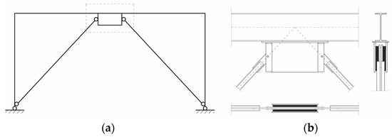
Figure 1.
(a) Schematic representation of a braced bay and (b) particular of the VED.
2. Dynamic Characteristics of Viscoelastic Materials
The response of a viscoelastic solid material to a shear deformation history γ(t) is intermediate between the response of an elastic solid material and a viscous fluid. If γ(t) is a harmonic function with amplitude γ0 and pulse ω, the steady-state stress response τ(t) of the VE material is lagged by a phase angle δ ranging from 0° (elastic behavior) to 90° (viscous behavior), i.e.,
The steady-state stress–strain hysteretic diagram described by Equations (1) and (2) has the shape of an ellipse centered on the origin and inclined with respect to the γ axe. The inclination of the ellipse depends on the elastic component of the response, while the enclosed area depends on the viscous component, as shown in Figure 2.
The hysteretic diagram of the VE material can be described by a pseudo-elastic law, i.e.,
where G* is called the “dynamic modulus”. This quantity accounts for both the elastic and viscous components of the response, whose contribution to the total response is a function of the phase angle δ. Equations (1) and (2) can be expressed in the frequency domain as follows:
The dynamic modulus is a complex number given by the following relation
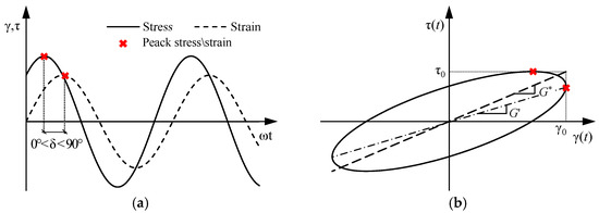
Figure 2.
(a) Mechanical response to cyclic deformation and (b) stress–strain diagrams for viscoelastic materials.
Figure 2.
(a) Mechanical response to cyclic deformation and (b) stress–strain diagrams for viscoelastic materials.
According to complex notation, the dynamic modulus can also be expressed in polar coordinates
or, equivalently, in Cartesian coordinates
where is called the “shear storage modulus” and represents the elastic component of the material behavior, whereas is called the “shear loss modulus” and represents the viscous components of the material behavior [13,35]. By equating Equations (7) and (8), and can be obtained
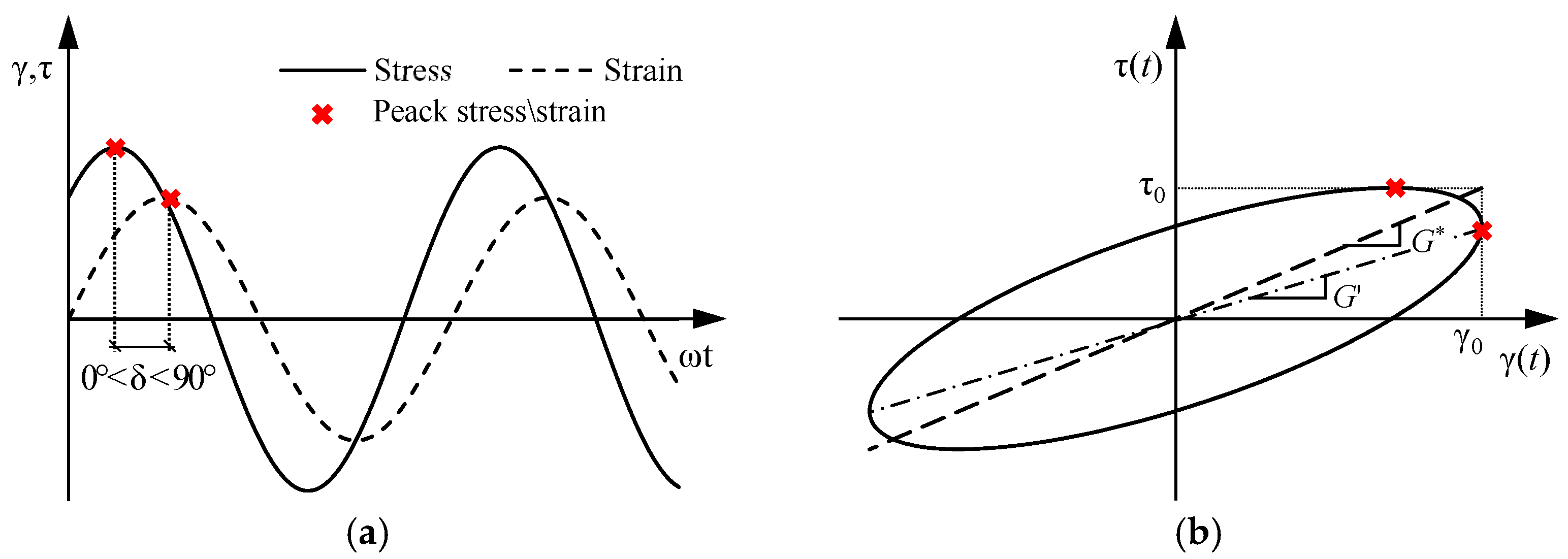
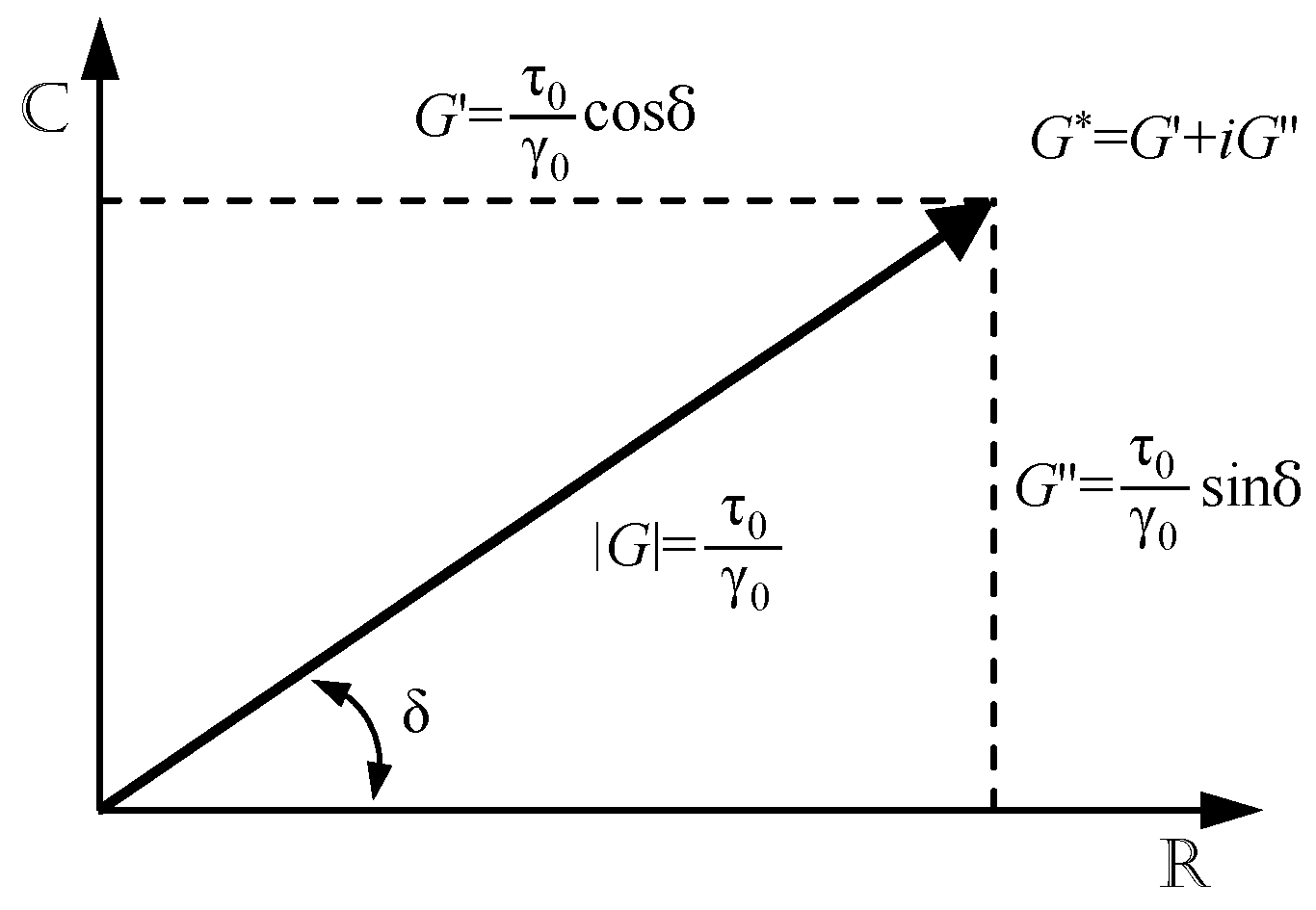
According to Equations (7) and (8), the dynamic modulus G* can be represented as a vector of the complex plane whose angle with the axis of the real numbers is the phase angle δ, as shown in Figure 3. The intensity of G* is called the “complex modulus” and is given as follows:
This mathematical representation is consistent with the actual behavior of VE materials. In fact, when the phase angle tends to 0° (elastic behavior), the loss modulus tends to zero. Vice versa, when the phase angle tends to 90° (viscous behavior), the storage modulus tends to zero. The ratio between the loss modulus and the storage modulus is called the “loss factor” η and represents an indicator of the damping capability of an elastomer [47]
Finally, the intensity of the dynamic modulus can also be expressed as a function of and
The complex modulus |G*|, the storage modulus , the loss modulus , and the loss factor η are the parameters that will be used in the next sections to characterize the elastomer.
Equation (3) can be rewritten in the frequency domain using Equations (4) and (5)
In the time domain, the above equation is expressed as
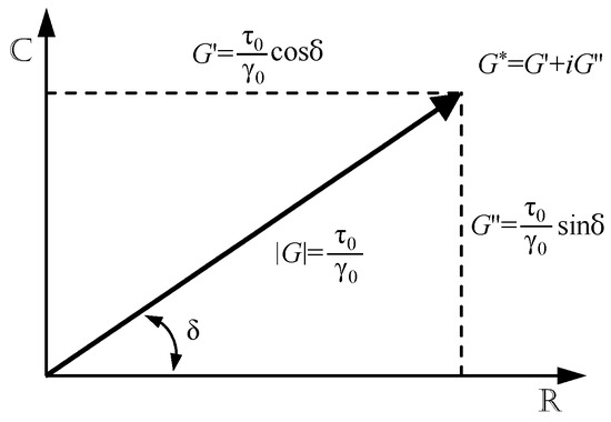
Figure 3.
Vectorial representation of the complex modulus G*.
Figure 3.
Vectorial representation of the complex modulus G*.
Considering the identity sin(α + β) = sinαcosβ + cosαsinβ, the Equation (15) can be rewritten as follows:
Considering Equations (9) and (10), it is possible to make the storage and the loss moduli explicit
Equation (17) is the constitutive equation of VE materials subjected to a harmonic loading with pulse ω and amplitude γ0. With further mathematical steps, Equation (17) can be rewritten as follows:
In this form, the constitutive equation represents the equation of an ellipse centered on the origin of the plane τ-γ and rotated by an angle that is equal to as shown in Figure 2b. The area enclosed by the ellipse represents the energy dissipated per cycle, i.e.,
Making the functions and explicit and considering Equation (17) and the first derivative of Equation (1) with respect to time yields
Note that the energy dissipated per cycle is proportional to the loss modulus only. Also note that according to Equations (18) and (21), if tends to zero, the ellipse collapses to a straight line with slope (elastic behavior), while if tends to zero, the axes of the ellipse match with the γ and τ axes (viscous behavior).
3. Numerical Model of Viscoelastic Dampers
The storage modulus and the loss modulus control the shape of the hysteretic cycle of a VE material. The dependency of the VE material on the load frequency, ambient temperature, and self-heating is then reflected on these parameters. As an example, the dependency of the storage modulus and the loss modulus on strain rate and ambient temperature is shown in Figure 4 for the elastomer ISD-110 tested by Chang et al. [8] for different load frequencies and with the control of the ambient temperature.
The dependency of and on strain rate is due to the molecular structure of elastomers: the faster the strain is applied, the less time molecular chains have to unroll.

Figure 4.
Variation of (a) the storage modulus G’ and (b) the loss modulus G” of the elastomer ISD-110 tested by Chang et al. [8] for rising frequency measured at different temperatures.
Figure 4.
Variation of (a) the storage modulus G’ and (b) the loss modulus G” of the elastomer ISD-110 tested by Chang et al. [8] for rising frequency measured at different temperatures.
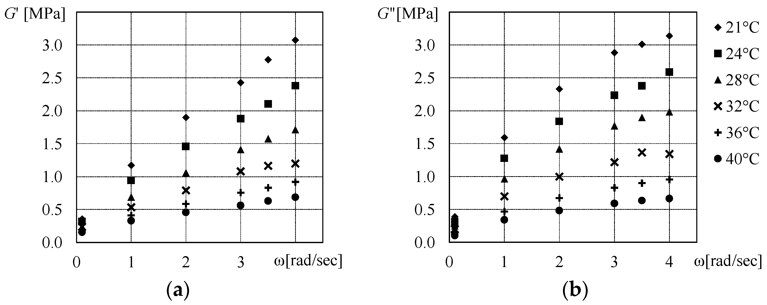
Therefore, an increase in the strain rate determines an increase in the stiffness and dissipative capability, i.e., an increase in both the storage modulus and the loss modulus. Variations in the ambient temperature affect both the stiffness and dissipation capabilities of the elastomer. An increase in ambient temperature magnifies the rubbery behavior of the material, and both the storage modulus and the loss modulus decrease. Similarly, self-heating of the elastomer due to prolonged operating times (e.g., in the case of wind excitation) decreases the storage and loss moduli.
In this paper, the strain rate dependency of the VE material is considered explicitly in nonlinear dynamic analyses through the VE material model introduced in this section. The effects of ambient temperature are taken into account by choosing experimental values of and and and obtained for a selected value of the ambient temperature. The effects of the temperature variation (due to self-heating) on and are neglected in this study. Indeed, the impact of self-heating on the mechanical properties of the elastomer in the case of short-duration events, like earthquakes, is considered negligible by some researchers [12,19,48]. Other researchers consider self-heating by means of the explicit calculation of the heat generated in the VE material during the loading history [27,49]. The resulting temperature variation is then used to evaluate new values of the storage and loss moduli through appropriate shift functions [11,49,50] (i.e., functions that provide the values of and depending on temperature and based on the time–temperature superposition principle). However, this process is not straightforward since it requires updating the material parameters during the numerical analysis. Moreover, this method requires the knowledge of additional properties of the selected VE material (e.g., specific heat capacity, time–temperature superposition functions) that are not always available in the literature.
The most common approaches in the literature for the numerical representation of VE materials are linear models (also referred to as integer derivative models) [2,7] and fractional derivative models [27,50,51].
Linear models are constituted by basic elements, i.e., springs and dashpots in various configurations. The simplest possible arrangements of one spring and one dashpot generate the well-known Kelvin–Voight model and Maxwell model, i.e., models with one spring and one dashpot connected in parallel and in series, respectively [51]. Even if these models are both able to reproduce the elliptical hysteretic cycle of the VE material by means of two parameters (i.e., the stiffness of the spring and the viscous constant of the dashpot), these simple models do not catch the strain rate dependency of the elastomer effectively. However, if more complex models are considered (i.e., with a larger number of parameters), the strain rate dependency of the elastomer may be effectively taken into account. The Generalized Maxwell Model, an in-parallel combination of more than one (n) Maxwell elements plus one Kelvin–Voight element (n + 2 parameters), is considered to be an effective solution for the representation of the strain rate dependency of VE materials [49,52,53].
Fractional derivative models are based on a basic discrete element called a “spring-pot”. The stress–strain behavior of this latter element is expressed through a linear differential operator that allows a differentiation of order α, α being either an integer or a fraction. When α = 0 or α = 1, the spring-pot is equal to a spring or a dashpot, respectively. When 0 < α < 1, a viscoelastic behavior is obtained. Like linear models, the use of the spring-pot element in combination with spring elements generates more complex models that effectively predict the response of VE materials. The advantage of such models is represented by the possibility of reproducing the VE behavior with a lower number of elements than linear models. Standard-linear solid models, i.e., models with a Kelvin–Voight element in series with a spring or models with a Maxwell element in parallel with a spring (3 parameters + the value of α), are considered to be valid solutions [54]. However, the spring-pot element is not available in the material library of most commercial software, including OpenSees v. 3.6.0, which is used to carry out the numerical analyses of this paper. Since the implementation of the spring-pot element is beyond the scope of this work, linear models are preferred herein.
In the following subsections, the models that are able to represent the VEDs are discussed. In particular, the Generalized Maxwell Model, to be used in nonlinear dynamic analysis and the equivalent brace model to be used in response spectrum analysis, are described.
3.1. Generalized Maxwell Model
In this study, the VE material is represented by means of a Generalized Maxwell Model with four Maxwell elements. The optimal number of Maxwell elements has been established based on the best trade-off between the number of parameters of the model and its effectiveness in reproducing the hysteresis cycles of the selected VE material at different frequencies. A schematic representation of the Generalized Maxwell Model with n = 4 (GMM4) is shown in Figure 5. The constitutive equation of the GMM4 is given as follows:
where and are the shear storage modulus and the shear loss modulus, respectively. These parameters are obtained by means of the following expressions
where
In the above equations, λi is the “relaxation time” of the material, GE,i and GC,i are the elastic modulus of the spring and the viscous coefficient of the dashpot of the i-th Maxwell element, GE,0 and GC,0 are the elastic modulus of the spring and the viscous coefficient of the dashpot of the Kelvin–Voigt element, and ω is the circular frequency of excitation of the structure (to be taken equal to the oscillation frequency of the structure in the fundamental mode of vibration). Details about the derivation of Equations (22)–(24) are reported in Appendix A. Note that both the storage and the loss moduli depend on the frequency of oscillation. Based on experimental values of and at various frequencies and fixed ambient temperatures, it is possible to calibrate the storage and loss moduli of the GMM4 model in order to reproduce the hysteretic behavior of the selected VE material. In this study, the elastomer ISD-111H tested by Montgomery [52] is considered. Experimental values of and obtained through cyclic tests at an ambient temperature of 20 °C and at frequencies of 0.1 Hz, 0.3 Hz, 1.0 Hz, and 2.0 Hz are shown in Table 1, together with the loss factor η.
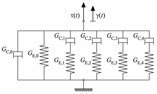
Figure 5.
Schematic representation of the Generalized Maxwell Model with four Maxwell elements (GMM4).
Figure 5.
Schematic representation of the Generalized Maxwell Model with four Maxwell elements (GMM4).

Calibration of the coefficients in Equations (23) and (24) is obtained through least square regression analysis performed on the data reported in Table 1 by means of the MS-Excel solver. The values obtained for the ten constants GE,0, GC,0 and GE,i, GC,i (with i = 1 to 4) of the GMM4 model are reported in Table 2.

Table 2.
Parameters of the GMM4 obtained by optimizing the equations of G’ and G” on experimental values.
Table 1.
Experimental values of the storage and loss moduli obtained for the elastomer ISD-111HH at 20 °C [52].
Table 1.
Experimental values of the storage and loss moduli obtained for the elastomer ISD-111HH at 20 °C [52].
| γ0 = 100% | f [Hz] | |||
|---|---|---|---|---|
| 0.1 | 0.3 | 1.0 | 2.0 | |
| G’ [MPa] | 0.123 | 0.191 | 0.327 | 0.446 |
| G” [MPa] | 0.101 | 0.183 | 0.366 | 0.517 |
| η [-] | 0.82 | 0.96 | 1.12 | 1.16 |
Equation (22) is expressed in terms of stress and strain. However, for design purposes, it is convenient to consider a force–displacement formulation in order to take account of the geometric characteristics of the VED
where and are called the “in-phase stiffness” and the “out-of-phase stiffness” of the VED, respectively. These parameters are obtained by means of the following relations
where Al and tl are the area and the thickness of a single elastomeric layer of the VED and nl is the number of layers.
3.2. Equivalent Brace Model
Since the proposed design procedure is based on linear elastic analyses (lateral force method of analysis and response spectrum analysis), only the contribution of the VED–brace subassembly to the lateral stiffness of the frame needs to be represented in the structural model. The VED is modeled as a simple spring whose stiffness corresponds to the in-phase stiffness of the VED at the expected ambient temperature and at the frequency corresponding to the dominant mode of vibration of the structure. The VED–brace subassembly is modeled as a single rod whose lateral stiffness is equal to that of the subassembly. Specifically, the lateral stiffness keq of the equivalent brace is obtained by the in-series sum of the lateral stiffnesses k’v of the VED and the lateral stiffnesses kb of the brace.
Referring to the schematic representation of the VED–brace subassembly shown in Figure 6, the lateral displacement utot of the node A due to a horizontal force F is given by the sum of the lateral deformation of the damper uv and the lateral deformation of the brace ub, i.e.,
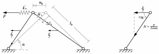
Figure 6.
Schematic representation of the brace–VED subassembly.
Both the VED and the bracing system are subjected to the force F. Therefore, the stiffnesses k’v and kb can be written as
where α is the angle of inclination of the brace with respect to the horizontal line, lb is the length of the brace, Ab is the area of the cross-section of the brace, and E is Young’s modulus of steel. Once the equivalent stiffness keq is determined by Equation (29), the VED–brace subassembly is represented in the numerical model by means of a fictitious brace with cross-sectional area Aeq equal to
4. Proposed Design Procedure
The proposed design procedure is based on the assumptions that (i) the response of the building equipped with VEDs is governed by the first mode of vibration and (ii) the addition of the VED–brace subassembly to the frame does not affect its first mode shape. Regarding the first hypothesis, Chang et al. [26] proved that the global response of a viscoelastically damped frame is essentially governed by the first mode o vibration. The second hypothesis derives directly from the application of the Modal Strain Energy method (MSE) as a design criterion [35,36,37,38]. Referring to this latter hypothesis, Tsai and Chang [37] demonstrated that the assumptions made in deriving the MSE method may result in an overestimation of the modal damping ratios of viscoelastically damped structures when the added damping is higher than 20%. Thus, these researchers recommended limiting the value of the added damping to a maximum value equal to 20%.
Due to its lateral deformability, the insertion of the VED–brace subassembly in the frame does not determine a significant increase in the lateral stiffness of the structure. Owing to this, beams and columns are sized according to capacity design rules established in Eurocode 8 [1] for steel moment-resisting framed (MRF) structures. Thus, members are verified according to Eurocode 3 [55] to resist internal forces determined by means of linear analyses. Once the MRF is fully sized, the VED–brace subassembly is included in the model and sized considering the effects of the higher modes of vibration. Finally, response spectrum analysis is performed to verify that limits on floor displacements are respected. The proposed design procedure is shown in the flowchart diagram reported in Figure 7.
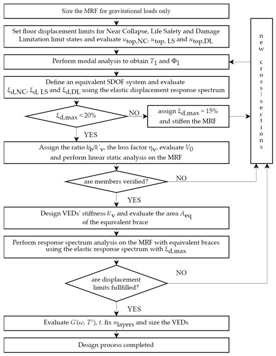
Figure 7.
Flowchart of the proposed design procedure.
Beams and columns of the MRF are designed for the Life Safety (LS) limit state (here associated with seismic events with a probability of exceedance of 10% in 50 years). Since limited damage is accepted in these members, the behavior factor q is taken equal to 1.5, the same value recommended in Eurocode 8 for base-isolated buildings.
To ensure the functioning of the dissipative system in the worst-case scenario, braces and the columns belonging to the braced bays are designed to remain elastic (q = 1) at the attainment of the Near Collapse (NC) limit state (here associated with seismic events with a probability of exceedance of 2% in 50 years). VEDs are designed to remain undamaged at the attainment of the NC limit state. The elastomer ISD-111H can totally recover from deformation of 400% without damage [56]. However, for the sake of safety (as no statistical data are available), VEDs are designed to develop a maximum deformation of 200% at the NC Limit State, as suggested by Kasai et al. [6].
4.1. Design of the MRF
In this study, the initial MRF is designed to sustain gravity loads only, according to prescriptions of Eurocode 3. Then, the modal analysis is performed, and the first period T1, the first mode shape Φ1, and the modal participation factor Γ(1) are obtained.
Limits on inter-story drifts δmax are established for Near Collapse (NC), Significant Damage (SD), and Damage Limitation (DL) limit states using the limits reported in FEMA 365 [57] as reference values for the corresponding limit states (i.e., Collapse Prevention, Life Safety, and Immediate Occupancy, respectively). These latter limits, reported in the first row of Table 3, are stipulated for the rehabilitation of existing MRFs. Since one of the objectives of the examined structural typology is to limit damage, it is reasonable to consider drift limits in the design of new buildings stricter than those reported in FEMA 365. Owing to this, the limit drift values adopted in this study are reported in the second row of Table 3.
Table 3.
Drift limits provided by FEMA 365 for MRFs for the considered limit states, and drift limits assumed for viscoelastically damped MRFs.
For the considered limit states, the maximum accepted values of the top displacement , , are calculated assuming that the drift limit is attained at all floors simultaneously. Then, the top displacements are converted into the displacements of equivalent SDOF systems , and using the following expression
where is the component of the first mode shape at the top floor.
For the considered limit states, the minimum demanded values of the equivalent viscous damping ratio, ξd,NC, ξd,LS, and ξd,DL, are evaluated by means of the elastic response spectrum scaled at the peak ground acceleration (PGA) corresponding to earthquakes with probability of exceedance equal to 2% (NC), 10%(SD), and 63% (DL) in 50 years, respectively. The values of ξd,NC, ξd,LS, and ξd,DL are found by minimization of the difference between the spectral ordinates Sd(T1, ξd,NC)ag,NC, Sd(T1, ξd,LG)ag,LG, and Sd(T1, ξd,DL)ag,DL, and the maximum displacements , , and of the equivalent SDOF system. The value of the equivalent viscous damping ratio to be considered in the next steps of the procedure is the maximum among the values determined for the considered limit states, i.e., ξd = max{ξd,NC, ξd,LS, ξd,DL}.
The equivalent viscous damping ξadd that shall be provided by the VEDs is equal to ξd minus the inherent damping ξ0 of the bare frame, assumed equal to 3% for steel MRFs.
For the sake of simplicity, the seismic base shear and the internal forces are obtained by means of the elastic response spectrum scaled at the PGA associated with the LS limit state. The behavior factor q and the importance factor γNC will be applied to the relevant members when internal forces are combined. The importance factor is calculated for the relevant limit state using the following expression, as suggested in Eurocode 8 Part 1 (§2.1 (4))
where PL is the probability of exceedance of the seismic action (2% and 63% in the case of NC and DL, respectively) in TL years (i.e., 50 years), PLR is the reference probability of exceedance (10% in the case of LS) over the same TL years, and k = 3 is a constant.
The design base shear is calculated by means of the following expression, as reported in Eurocode 8
where Se(T1, ξ0)ag,LS is the spectral acceleration obtained at the period of vibration T1 for the equivalent viscous damping ratio ξ0 of the bare frame, m is the seismic mass of the building, and λ is a correction factor (=0.85) accounting for the difference between the base shear force predicted by the lateral force method of analysis and the response spectrum method of analysis.
The base shear obtained by Equation (36) is reduced based on the MSE method, as shown in the following steps. According to the MSE method, the equivalent viscous damping ratio of the damped structure can be expressed as
where ηv-b is the loss factor of the damper–brace subassembly, K0, Ks, and Kv-d are the lateral stiffness of the MRF, the lateral stiffness of the damped structure, and the lateral stiffness of the damper–brace subassembly, respectively. Assuming that the base shear is proportional to the lateral stiffness of the structure, Equation (37) can be rewritten as [36]
where Vv-d is the fraction of Vbase to be sustained by the dissipative system and V0 is the fraction to be resisted by the MRF. The value of the seismic base shear to be used to design the MRF is then derived from Equation (38) as
where B is a corrective coefficient (equal to ) of the equivalent viscous damping ratio given in Eurocode 8 Part 1-1 (§3.2.2.2).
The loss factor of the VED–brace subassembly, ηv-b, is given by the subsequent expression [6,36]
where kb is the lateral stiffness of the brace and k’v is the lateral stiffness of the VED. The loss factor of the elastomer (i.e., the ratio of the loss modulus to the storage modulus) is a stable quantity with respect to both frequency and temperature and for the elastomer ISD-111H, it can be assumed equal to unity. The ratio kb/k’v is a design parameter that has to be established a priori and denotes how stiff the brace is with respect to the lateral stiffness of the VED. Clearly, the stiffer the brace, the higher the deformation of the VED. Chang et al. [36] found that the efficiency of the dissipative system is sensitive to the ratio kb/k’v up to a value of 40. Further increases in the lateral stiffness of the brace do not improve the performance of the VEDs significantly.
The base shear V0 is used to perform a linear static analysis on the initial MRF and obtain the internal forces due to seismic action. In this phase, the behavior factor q and the importance factor γNC are applied. The resulting internal forces are combined with the internal forces due to gravity loads in the seismic combination and the resistance and lateral stability checks are conducted on members of the MRF and on the dissipative systems. If beam and column cross-sections need to be changed, the above steps of the procedure are iterated until each member of the structure is verified.
Note that if the period of the initial structure falls into the constant-displacement zone of the spectrum and numerous iterations are required to complete the design process, the structure might become increasingly rigid, and the demanded damping might decrease at each iteration. In such a case, some judgment is necessary to obtain a rational design. A viable strategy is to fix a value of ξadd that is greater than or, at least, equal to ξd − ξ0 and lower than 20%—ξ0 at the very first iteration and benefit from the reduction of the base shear. Once fixed, the value of ξadd shall no longer be modified. Chang et al. [36] suggested an initial value of ξadd equal to 15%, regardless of the limits on drifts.
4.2. Design of the Braces
In accordance with Equation (38), the design value of the lateral stiffness of the VED-brace subassembly at the i-th floor, kv-b,i is given as follows:
where
where k0,i is the lateral stiffness of the MRF at the i-th floor. The stiffness of the VED at the i-th floor is given by the subsequent expression [36]
Recall that the response of the VEDs is sensitive to the changes in the load frequency. Thus, the force that arises in VEDs and that is transferred to the braces is affected by the higher modes of vibration. Further, due to the phase shift of the VE material, the force associated with the maximum displacement through the stiffness k’v,i is not the maximum force that occurs in the device (see Figure 2b). To obtain an accurate prediction of the maximum axial force in braces due to seismic actions, the following steps are required in the design process.
First, an initial value of the lateral stiffness kb,i of the braces at the i-th floor is estimated from the prefixed ratio kb/k’v considering the value of k’v,i calculated by Equation (43). The calculation of the lateral stiffness and the cross-sectional area of the equivalent brace by Equations (29) and (33) is straightforward. The structural model is then updated, including the equivalent braces modeled as hinged rods with area Aeq.
Secondly, the period of vibration Tj and the seismic lateral forces Fi(j) associated with the j-th mode are determined by modal analysis of the MRF with equivalent braces. Then, the in-phase stiffness of the VE material is calculated for each mode of vibration by Equation (23) considering the respective circular frequency. If are the stiffnesses of the VEDs in the first mode of vibration, the stiffnesses of the VEDs corresponding to the j-th mode (with j > 1) are calculated through the following expression
The stiffnesses and the areas of the equivalent braces are evaluated by Equations (29) and (33) for each mode of vibration. For the j-th mode of vibration, the axial forces in braces are obtained by linear static analysis performed on the structure with equivalent braces with area using the equivalent seismic forces Fi(j).
Third, the axial forces obtained in braces for the j-th mode are multiplied by a corrective factor that accounts for the shift between the occurrence of the maximum deformation and maximum force in VEDs
The maximum axial forces in the braces due to seismic action are finally obtained, combining the effects of the modes of vibration using the SRSS rule. As braces are expected to remain elastic at the NC limit state, the importance factor γNC is applied, i.e.,
The axial forces in braces due to gravity loads () in the seismic combination are computed through a separated analysis performed on a different structural model. Specifically, braces are modeled with their effective cross-section to account for the fact that, in the vertical direction, the stiffness of the braces is not affected by the presence of the VED. At the first iteration, the cross-section of the brace at the i-th floor is chosen so that its lateral stiffness kb,i is greater or equal to the lateral stiffness of the VED k’v times the prefixed ratio kb,i/k’v.
Note that even if the design of the braces may require more than one iteration, the stiffness of the VED–brace subassembly always remains low compared with the lateral stiffness of a real brace. Thus, the insertion of the VED–brace subassembly in the MRF does not affect the period of the structure significantly (i.e., no further iterations are necessary to verify the members of the MRF).
4.3. Check on Drift Limits
Once all members of the structure are sized, the model is updated considering the equivalent braces, and a response spectrum analysis is performed to check that the limits on drifts are not exceeded on all floors. The analysis is run using the elastic response spectrum scaled at the PGA corresponding to the LS limit state and considering the viscous damping ratio ξd. The resulting floor displacement profile is compared with the maximum displacement profile derived from the limits reported in Table 3 for the LS limit state. The displacement profiles corresponding to NC and DL limit states are obtained by multiplying the components of the LS displacement profile by the respective importance factors γNC = 1.71 and γDL = 0.472.
4.4. Design of the VEDs
Once the design of the MRF is complete and the assumed limits on floor displacement are verified, the thickness tl, the areas Al,i, and the number nl of the elastomeric layers of the VEDs are determined.
The thickness tl is given as the ratio of the maximum allowed floor displacement Δumax,NC to the maximum allowable strain established for the elastomer at the NC limit state (i.e., 200%)
where Δumax,NC is given as
where h is the interstory height.
To mitigate the self-heating of the VEDs in the case of long-duration events, Kasai et al. [27] suggested considering elastomeric layers thicker than 12.7 mm. In this study, this value is considered as a lower bound for the thickness of the elastomeric layers.
Finally, the area of the elastomeric layers Ai,l of the damper at the i-th floor is given by the following expression:
The storage modulus G’ (ω1, Temp) of the elastomer is evaluated by Equation (23) considering the circular frequency of the first mode of vibration of the structure and the established service temperature.
5. Application to a Case Study
The procedure illustrated in the previous section is applied to design a set of twelve residential buildings with 4, 6, and 8 stories, located in a medium or high seismicity zone with reference PGA ag,R equal to 0.25 g or 0.35 g founded on rock soil (type A soil according to Eurocode 8 Part 1) or soft soil (type C soil).
All buildings have the same squared floor plan whose axes of symmetry lay in the X and Y directions, as shown in Figure 8. The structure consists of two sets of four steel MRFs arranged in two orthogonal directions. The length of the bays is equal to 8 m in both directions, and the inter-story height is equal to 3 m at all levels. VEDs are located at all stories in the central bay of each perimetral frame, sustained by a couple of braces in the chevron configuration and connected to the bottom flange of the beam. Columns of the MRF are denoted with the letter “C” and a number that is 0 for columns belonging to the braced bay, 1 for corner columns, and 2 for columns of the central part of the building. Columns C0 are oriented with the strong axis perpendicular to the plane of the braced bay, columns C1 are oriented with the strong axis parallel to the X direction, and columns C2 are oriented with the strong axis parallel to the Y direction. HEB profiles are used for columns and braces, whereas IPE profiles are used for beams. To minimize the weight of the structure, different steel grades are used, i.e., steel grade S355 is used for columns, S275 is used for beams, and S235 is used for braces. Bi-directional slabs are used in order to equally distribute gravity loads on the beams. It is assumed that slabs are rigid in their plan and that masses are equally distributed over the floor surface.
Characteristic values of dead loads gk and live loads qk acting on the slabs are assumed to be equal to 4.40 kN/m2 and 2.00 kN/m2, respectively. The design gravity loads in the non-seismic and seismic design situations are equal to 9.16 kN/m2 and 5.00 kN/m2, respectively. The values of the line loads applied to the beams and the values of the axial forces applied to the columns are determined as a function of tributary areas. The value of the floor masses is equal to 146.8 t at all floors.
In the following sections, the application of the proposed procedure is developed in detail for the 4-story building founded on rock soil (A) in an area characterized by medium seismic hazard (PGA = 0.25 g).
5.1. Numerical Model for Design Analyses
Due to the in-plan and in-elevation regularity of the buildings, a two-dimensional numerical model is considered. Further, due to the double symmetry of the plan, only a perimetral and a central frame are included in the model, as shown in Figure 9. To simulate the rigid diaphragm effect due to the slabs, all the nodes of the two frames belonging to the same floor are constrained to have the same translational displacements. All members are modeled as elastic elements.
Columns are constituted by the same profile along the height of two stories and column-to-column connections are assumed to be rigid and full-strength. Column-to-foundation connections are fixed, except for the case of C0 columns, which are pin-connected to the foundation. With the sole exception of the braced beam, which is pinned at the ends, beams-to-columns connections are fixed.

Figure 8.
Floor plan of the case studies.
Figure 8.
Floor plan of the case studies.
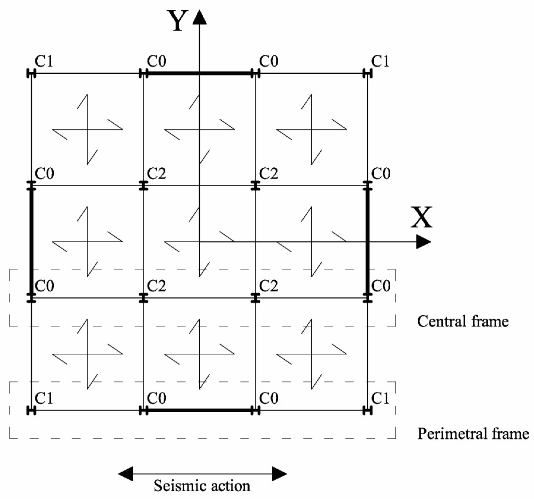
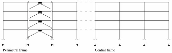
Figure 9.
Schematic representation of the plane model.
Figure 9.
Schematic representation of the plane model.
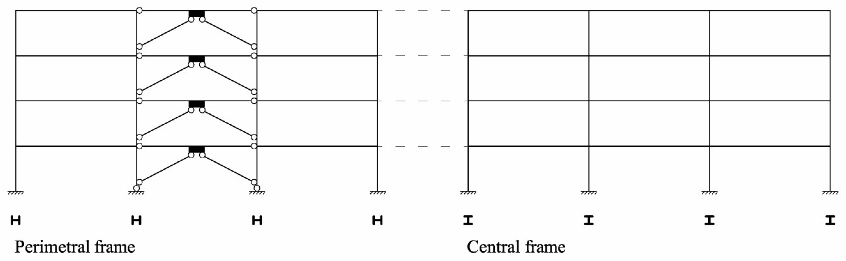
In the model to use for design analyses, the VED–brace sub-assemblage consists of two truss members in the chevron configuration. Note that in the horizontal direction, the stiffness of the VED–brace assemblage is given by the equivalent brace model discussed in Section 3.2, while in the vertical direction, the stiffness of the VED–brace assemblage is the same as the stiffness of the sole braces. Thus, to properly estimate the axial force in the braces, internal forces due to gravity loads in the seismic combination and due to seismic actions are separately evaluated considering two different structural models. In the model for gravity loads analysis, the actual cross-section of the chosen steel profile is used for braces. In the model for response spectrum analysis, the cross-sectional area of the braces is evaluated using the equivalent brace model. Internal forces resulting from the two structural models are then combined.
The seismic action is represented by the average elastic response spectrum obtained from artificial ground motion records for different values of the equivalent viscous damping ratio ξ, namely 3%, 5%, 10%, 15%, and 20% of the critical damping. Spectra corresponding to intermediate values of ξ are obtained by linear interpolation. The set of 10 artificial ground motions used to generate the spectra is the same set used to perform nonlinear dynamic analyses (NLDA) and discussed in Section 6. The use of average spectra instead of the EC8 spectrum is preferred to simplify the comparison with the results of NLDA.
5.2. Design of the MRF
The initial MRF is sized to sustain gravity loads only in the non-seismic situation. Beam and column cross-sections obtained from gravity loads analysis are shown in Table 4. Then, modal analysis is performed on the initial MRF and the period T1, the mode shape Φ1 and the modal participation factor Γ(1) associated with the first mode of vibration are obtained. The minimum values of the required equivalent viscous damping ratio are determined for NC, LS, and DL limit states based on the prefixed drift limits established in Section 4.1 (see Table 3). These values are shown in Table 5.
Table 4.
Cross-sections of beams and columns obtained through gravity load analysis.
Table 5.
Minimum values of the required equivalent viscous damping ratio for the considered limit states.
The damping ratio that should be provided by the dampers is equal to
The ratio kb/kv is assumed to be equal to 40, and the loss factor ηv of the elastomer ISD-111H is taken equal to 1. The reduced value of the seismic base shear V0 is evaluated by Equation (39) considering the spectral acceleration Se(T1, ξ0)ag,LS. Internal forces due to seismic actions are determined by the lateral force method of analysis. The value of the reduced seismic base shear V0 and the other quantities involved in the calculations are shown in Table 6 for the first and the last design iteration. It should be noted that V0 is about 80% Vbase.
Table 6.
Values of the design base shear at the first and at the last iteration on the procedure and relevant quantities for the calculations.
Capacity design rules are applied to size the elements of the frame. Beam and column cross-sections obtained at the last iteration are shown in Table 7.
Table 7.
Cross-sections of beams and columns obtained at the last iteration of seismic analysis.
5.3. Design of the Braces
The lateral stiffness of the VED–brace subassembly is calculated at each story as a function of ξd by Equation (41). The lateral stiffness of the VEDs is then calculated by Equation (43).
Since the lateral stiffness of the VED–brace subassembly at the i-th story is proportional to the lateral stiffness of the frame at the i-th story by means of the factor αMSE, the hypothesis that the first modal shape remains unaltered is fulfilled. The values of kv-b,i and kv,i and the relevant quantities needed for their calculation are shown in Table 8.
Once the lateral stiffness k’v.i of the VED–brace subassembly has been determined at all floors, the lateral stiffness kb,i of the braces can be calculated through the ratio kb/k’v, and a minimum cross-section of the braces can be determined.
Table 8.
Lateral stiffnesses of the VED–brace subassemblies and of the VEDs and other relevant quantities.
Table 8.
Lateral stiffnesses of the VED–brace subassemblies and of the VEDs and other relevant quantities.
| Piano | αMSE [-] | k0,I [kN/mm] | kv-b,I [kN/mm] | k’v,I [kN/mm] |
|---|---|---|---|---|
| 1 | 0.162 | 21.599 | 3.490 | 3.494 |
| 2 | 17.824 | 2.880 | 2.883 | |
| 3 | 12.767 | 2.063 | 2.065 | |
| 4 | 11.777 | 1.903 | 1.905 |
To consider the effects of the higher modes of vibration on the mechanical properties of the VEDs, the axial forces in braces are evaluated according to the procedure illustrated in Section 4.2., i.e., a response spectrum analysis is performed on the structure with equivalent braces, and the lateral forces Fi(j) associated with the j-th mode are memorized. The reference spectrum is the artificial elastic spectrum scaled at a PGA = 0.25 g with an equivalent viscous damping ratio equal to ξd = 9.62%. For each mode of vibration, a linear static analysis is performed using a distribution of forces proportional to the relevant mode of vibration. The values of the axial forces obtained from each analysis for the braces are then combined using the SRSS rule according to Equation (46) and then combined with the axial forces due to gravity loads in the seismic combination. The resulting value of the axial force is used to design the braces. If the checks on resistance and/or lateral stability are not fulfilled, a new cross-section is selected, and the analysis is repeated until convergence has been reached. The cross-sections of the braces at the first and last iterations of the procedure are shown in Table 9.
Table 9.
Cross-sections of the braces (S235) at the first and last iteration.
5.4. Check on Drift Limits
Once the MRF and the braces are sized, a response spectrum analysis is performed on the frame with equivalent braces to verify whether the limits on drifts are met at all floors. The reference response spectrum is the elastic response spectrum scaled at a PGA = 0.25 g with ξd = 9.62%.
Limits on floor displacements are fulfilled for all the considered limit states. The first period of the final structure with equivalent braces is T1 = 1.548 s. Note that the period of the MRF without the equivalent braces is equal to 1.668 s, i.e., the presence of the equivalent braces decreases the period by about 7%.
5.5. Design of the VEDs
Once the structure with equivalent braces has been designed and the final period of vibration is known, the thickness and the minimum required area of the elastomeric layers of the dampers can be evaluated. The thickness of the elastomeric layers is calculated by Equation (47) considering the maximum floor displacement allowed for the conditioning limit state (i.e., Significant Damage). Considering that VEDs are allowed to reach their maximum deformation at the attainment of the NC limit state, the maximum displacement for the SD limit state is amplified by the importance factor γNC
The value of the storage modulus is evaluated by Equation (23) for the circular frequency ω1 corresponding to the final value of the period T1 and considering a temperature of 20 °C.
The number of elastomeric layers is a design parameter that is established depending on the desired size of the device. The areas of the elastomeric layers can be determined at all stories using Equation (49). In this example, the areas of all VEDs are determined considering four rectangular layers of elastomer. The dimensions bl × hl of each layer are obtained by fixing one of the two dimensions of the layer (hl = 20 cm in this example). The relevant quantities needed for the sizing of the VEDs are shown in Table 10.
The final cross-sections of the members and the final dimensions of the VEDs of the other buildings are shown in Appendix B.
Table 10.
Areas and dimensions of the elastomeric layers and relevant quantities for the calculations.
Table 10.
Areas and dimensions of the elastomeric layers and relevant quantities for the calculations.
| Floor | T1 [s] | G’ [N/mm2] | t [mm] | nl | Al,i [cm2] | bl × hl [cm] |
|---|---|---|---|---|---|---|
| 1 | 1.548 | 0.268 | 25.7 | 4 | 838.80 | 42 × 20 |
| 2 | 692.19 | 35 × 20 | ||||
| 3 | 495.79 | 25 × 20 | ||||
| 4 | 457.38 | 23 × 20 |
6. Nonlinear Dynamic Analyses
The seismic response of the structures designed through the proposed procedure is evaluated by nonlinear dynamic analyses considering P-Δ effects. Numerical analyses are performed by means of the OpenSees v. 3.6.0 computer program [58].
The seismic input consists of two sets of 10 artificial accelerograms generated for a PGA equal to 0.35 g with the computer program SIMQKE [59] to match the elastic response spectrum with 5% equivalent viscous damping provided by Eurocode 8 for soil type A or C.
The two-dimensional structural model of the MRF has the same geometrical characteristics and boundary conditions as the model used for design analyses. Under the same assumptions formulated in Section 5.1, only two frames of the structure are modeled (i.e., a perimetral frame and an inner frame). The presence of rigid slabs is simulated by means of constraints applied at each floor between a master node belonging to the perimetral frame and the other nodes belonging to the same floor to force the constrained nodes to have the same horizontal displacements. All members are represented by a single force-based element, except for the beams of the braced bay that are modeled with two elements to have a node at midspan for the connection with the VEDs.
Members of the MRF that are expected to develop plastic hinges (i.e., C1-, C2-columns and beams) are modeled as forceBeamColumn elements with fiber sections and elastic interior. The length of the plastic hinges is assumed to be equal to the height of the member cross-section. The integration method for the plastic hinge is “HingeRadau”. Members that are expected to remain elastic at the attainment of the NC limit state (i.e., braces and C0-columns) are modeled as elasticBeamColumn elements.
Each VED is modeled using six zeroLength elements connected in series between a node belonging to the braces and the midspan node of the beam of the braced bay. A uniaxialMaterialElastic, uniaxialMaterialViscous, and uniaxialMaterialViscousDamper are assigned to the zeroLength elements representing the spring, the dashpot, and the Maxwell elements of the GMM4 model (see Figure 5), respectively. The parameters that characterize the response of the single springs and dashpots of the GMM4 are calculated using the following relations
where kEi,n and cci,m are the stiffness and viscous coefficients of the n-nth spring and m-nth dashpot of the model (n, m = 0, 1, …, 4) at the i-th story; GE,n and Gc,m are the constants of the model as determined by the optimization on the experimental data of the elastomer ISD-111H (see Table 2). Ai, nl, and tl are the geometric characteristics of the VED. The calculated values of kEi,n and cci,m are shown in Table 11.
Table 11.
Values of the stiffness and of the coefficient of viscosity of the springs and the dashpots of the GMM4 model.
The Rayleigh formulation is used to introduce the inherent damping of the frame (mass and stiffness coefficients are defined so that the first and second modes of vibration are characterized by an equivalent viscous damping ratio equal to 0.03). No stiffness proportional damping is considered for the braces. Convergence of the numerical solution is checked in terms of the norm of the displacement increment with a tolerance of 10 × 10−6 over a maximum of 100 iterations. The initial integration step is 0.005 s. Three algorithms are used in sequence to reach convergence at the single step of the accelerogram (i.e., Newton Initial, Broyden, NewtonLineSearch). If convergence is not achieved with this strategy, the displacement step is reduced by half.
For each case study, an incremental NLDA is conducted starting from a PGA of 0.04 g to reach a PGA of 0.60 g with increment steps of 0.04 g. The subsequent response parameters are checked:
- The values of the PGA corresponding to the achievement of yielding, or buckling of the members of the MRF and to the limit displacement established for the VEDs;
- The lateral story displacements;
- The internal forces in the dampers, braces, and C0-columns.
6.1. Seismic Response of the Case Study
The achievement of yielding at the ends of the beams and/or at the base of the C1- and C2-columns (i.e., members designed considering q = 1.5) is expected for values of the PGA equal to or larger than 0.2 5 g/1.5 = 0.167 g. The members of the braced bay are expected not to develop internal forces associated with the plasticization of the cross-section or the buckling of the member until the value of the PGA associated with the NC limit state is reached. The elements of the braced bays, instead, are expected to remain elastic until the value of the PGA associated with the NC limit state has been reached, i.e., 0.25 g × 1.71 = 0.429 g. VEDs are expected to reach the maximum allowed deformation at the NC limit state (i.e., 200%) at the attainment of a story drift equal to 51.4 mm.
The numerical analysis shows that the damper located at the first story reaches the NC limit state first at a PGA equal to 0.443 g, which is slightly higher than the expected value (i.e., 0.429 g). Braces remain elastic and do not buckle even when the maximum expected value of the PGA (0.429 g) is reached. C0-columns remain elastic until the NC limit state of the structure has been reached.
The force–displacement responses of the VEDs recorded at a PGA equal to 0.443 g for one of the accelerograms are shown in Figure 10. The effects of the higher modes of vibrations are particularly apparent in the hysteretic cycles of the dampers located at the first and second story whose shape is irregular and not perfectly elliptical.
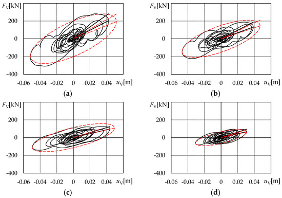
Figure 10.
Hysteretic cycles of the VEDs located at the first (a), second (b), third (c), and fourth (d) story recorded at the PGA of 0.437 g and enveloped by the GMM4 model for ω1 = 4.077 rad/s (i.e., T1 = 1.541 s).
However, the hysteretic cycles of the VEDs are well enveloped by the response of the GMM4 model calibrated based on the maximum forces and maximum displacements recorded in the dampers and considering the frequency associated with the first period of the structure (red dashed line in the figure).
The values of the maximum forces recorded in the dampers and the ratios of the maximum allowed displacement to the maximum displacement experienced are shown in Table 12. The latter data show that the dissipative system is efficient as almost all the dampers approach their maximum stroke during the time history.
Table 12.
Maximum forces and displacements reached by the VEDs for a PGA of 0.437 g corresponding with the achievement of the maximum deformation for the damper located at the first story.
As shown in Figure 11a, the average values of the axial force of C0-columns recorded with OpenSees are well predicted by the response spectrum analysis with ξ = 9.62%. The average values of the shear force and bending moment are slightly overestimated, as shown in Figure 11b,c. The average values of the axial force in braces are satisfactorily predicted by the SRSS analysis, even though the axial force is slightly underestimated at the first floor, as shown in Figure 11d.
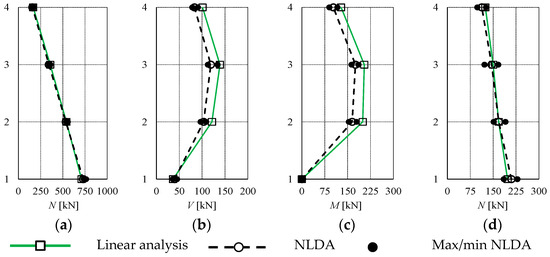
Figure 11.
(a) Axial forces, (b) shear forces, and (c) bending moments in C0 columns, (d) axial forces in braces (PGA = 0.429 g).
As part of the MRF, columns C1 and C2 are allowed to develop plastic hinges at their base, and this happens for an average value of PGA equal to 0.280 g. The average of the PGAs associated with the development of the first plastic hinge in a beam of the MRF is equal to 0.241 g. No significant difference is recorded between the design predictions and the results of dynamic analyses for the internal forces of the columns of the MRF.
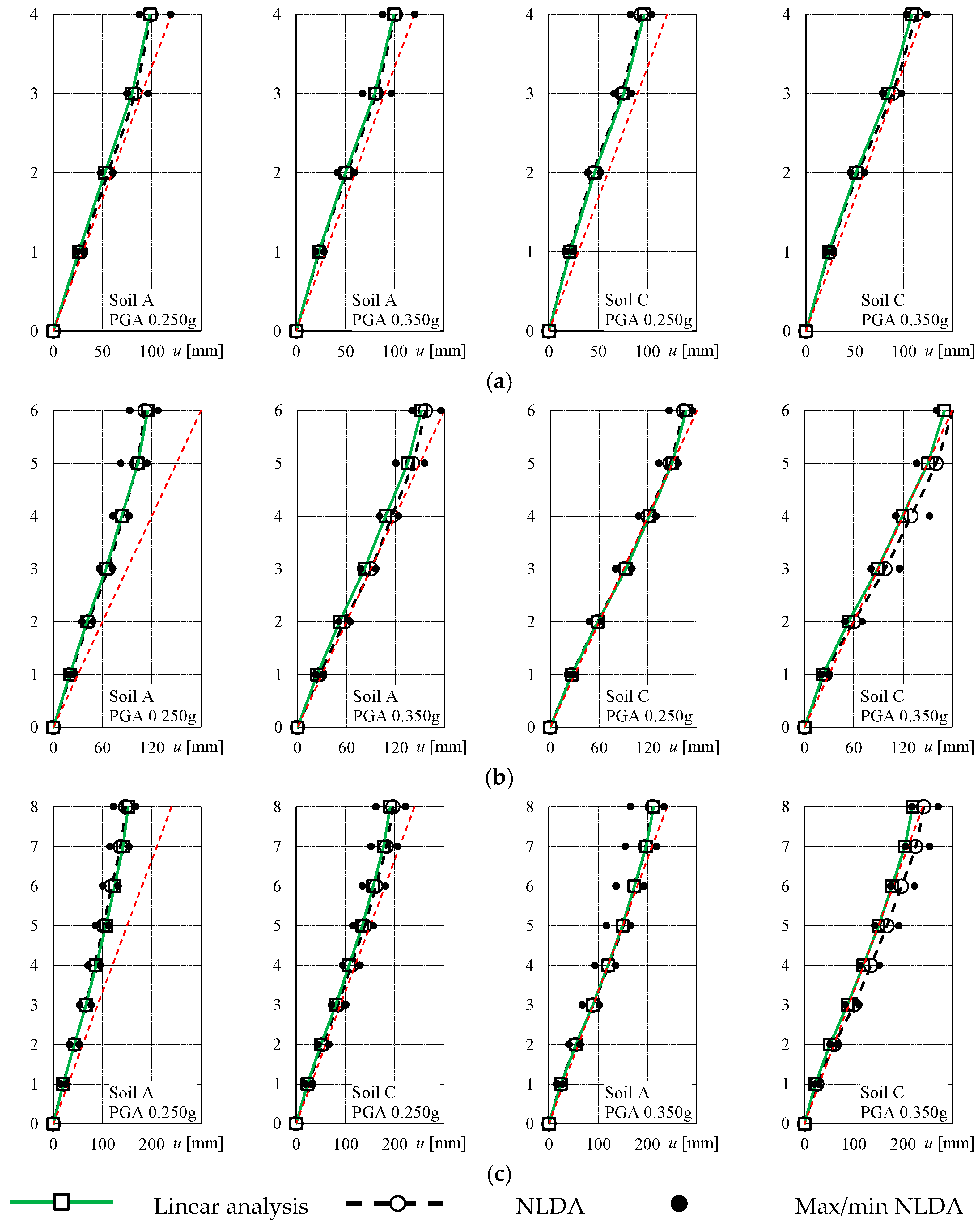
The comparison between the average floor displacements obtained by dynamic analysis for a PGA equal to 0.25 g and the displacements predicted by response spectrum analysis with ξ = 9.62% is shown in Figure 12. The design solution obtained through the proposed procedure fulfills the limitations on the floor displacements and the members are verified against the design internal forces.
6.2. Seismic Response of the Other Buildings
The values of the PGA corresponding to the first yielding in beams or columns of the MRF and to the first attainment of the maximum allowed deformations in the VEDs are shown in Table 13 for all the case studies. Also, the values of the expected PGA are reported for both SD and NC limit states. In the range of the investigated PGAs (i.e., 0.04 g–0.60 g), the internal forces associated with the plasticization of the cross-section or the buckling of the C0-columns or the braces are never attained. Braces and C0-columns always remain elastic.
Table 13.
Values of the PGA for which the SD limit state and the NC limit state are attained in members of the MRF and the VEDs.
Table 13.
Values of the PGA for which the SD limit state and the NC limit state are attained in members of the MRF and the VEDs.
| Case | PGASD | PGANC | PGAbeams | PGAcolMRF | PGAVED | |
|---|---|---|---|---|---|---|
| 4-story | Soil A | 0.250 | 0.429 | 0.241 | - | 0.443 |
| 0.350 | 0.600 | 0.309 | - | 0.603 | ||
| Soil C | 0.250 | 0.429 | 0.273 | - | 0.437 | |
| 0.350 | 0.600 | 0.340 | - | 0.541 | ||
| 6-story | Soil A | 0.250 | 0.429 | 0.330 | 0.312 | 0.544 |
| 0.350 | 0.600 | 0.341 | 0.386 | 0.572 | ||
| Soil C | 0.250 | 0.429 | 0.222 | 0.273 | 0.376 | |
| 0.350 | 0.600 | 0.292 | - | 0.513 | ||
| 8-story | Soil A | 0.250 | 0.429 | 0.304 | 0.361 | 0.505 |
| 0.350 | 0.600 | 0.353 | 0.432 | 0.560 | ||
| Soil C | 0.250 | 0.429 | 0.223 | 0.291 | 0.357 | |
| 0.350 | 0.600 | 0.281 | 0.372 | 0.489 | ||
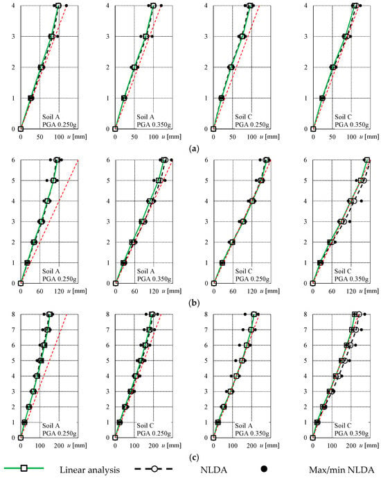
Figure 12.
Comparison between floor displacements predicted by response spectrum analysis and displacements obtained through NLDA for (a) four-, six- (b), and (c) eight-story buildings designed for A or C soil and for design PGA equal to 0.25 g or 0.35 g.
Figure 12.
Comparison between floor displacements predicted by response spectrum analysis and displacements obtained through NLDA for (a) four-, six- (b), and (c) eight-story buildings designed for A or C soil and for design PGA equal to 0.25 g or 0.35 g.
Dampers always reach the maximum allowed strain after the formation of the first plastic hinge in the MRF. In some cases, the value of the PGA associated with the first attainment of the maximum allowed strain in one of the VEDs is smaller than expected. This discrepancy is apparent in the cases in which the added damping is greater than 10%. However, it should be noted that these values of the PGA refer to only one damper (i.e., the first to reach the maximum strain), and thus, they do not refer to the whole dissipative system. Also, recall that the rupture of a VED occurs for values of the shear deformation of the elastomeric layer of about 400%, a value that is twice the assumed maximum deformation at the attainment of the NC limit state.
The observations formulated in the previous subsection for the case study regarding the prediction of the internal forces in the members of the MRFs, in C0-columns and in the braces, can be extended to the other buildings.
As shown in Figure 12, the assumed limits on the floor displacements are fulfilled in all the case studies.
7. Conclusions
In this paper, a design procedure for steel moment-resisting frames with viscoelastic dampers has been proposed. The parameters that control the response of viscoelastic materials, namely the storage modulus, the loss modulus, and the loss factor, have been discussed, and their dependency on frequency and ambient temperature has been pointed out. A simple and frequency-dependent numerical model, the Generalized Maxwell Model with four Maxwell elements (GMM4), has been proposed to represent the dynamic response of viscoelastic materials. Mathematical expressions for the storage and the loss moduli of the GMM4 have been derived analytically and calibrated based on experimental data of a commercial elastomer.
The proposed design procedure is based on the Modal Strain Energy (MSE) method, and its application requires simple analytical tools, such as the modal response spectrum analysis and the lateral force method of analysis. This approach has been improved in order to accurately predict the internal forces that are transmitted from each damper to the braces due to the sensitivity of the VE material to the effects of the higher modes of vibration.
The design procedure has been applied to 4-, 6-, and 8-story buildings equipped with viscoelastic dampers sustained by braces in the chevron configuration. The buildings are founded on different soils (Soil A and C) and are designed based on seismic actions of different intensities (design PGA equal to 0.25 g and 0.35 g).
To validate the proposed design procedure, the response of the designed buildings was investigated by nonlinear dynamic analyses. Based on the results of the NLDA, the following conclusions can be drawn:
- The fulfillment of the main design objective, i.e., the control of the story drifts below prefixed limits, is achieved for all cases. At the same time, the internal forces of the braces and of the other members of the MRF are well predicted. This proves the effectiveness of the procedure based on the MSE method.
- The GMM4 model is effective in reproducing the hysteretic behavior of the VEDs as a function of frequency and for a given ambient temperature.
- VEDs are effective in conferring the demanded damping to the structure, although in the cases in which high damping is demanded, at least one of the dampers of the dissipative system exceeds the maximum allowed displacement for a value of the PGA that is lower than the expected value.
Future developments of this research will concern:
- Optimal arrangement of the dampers in the structure;
- Comparison of the seismic performance and construction costs of the frames designed by means of the proposed procedure with those of the frames designed by means of other procedures available in the literature;
- Study of the response of viscoelastically damped structures in the case of near-fault design scenarios.
Author Contributions
Conceptualization, M.B., A.F. and P.P.R.; methodology, M.B., A.F. and P.P.R.; software, M.B. and A.F.; validation, M.B., A.F. and P.P.R.; formal analysis, M.B., A.F. and P.P.R.; investigation, A.F. and P.P.R.; writing—original draft preparation, A.F.; writing—review and editing, M.B., A.F. and P.P.R. All authors have read and agreed to the published version of the manuscript.
Funding
This research received no external funding.
Data Availability Statement
The data that support the findings of this study are available from the corresponding author, A.F., upon reasonable request.
Conflicts of Interest
The authors declare no conflicts of interest. The funders had no role in the design of the study, in the collection, analyses, or interpretation of data, in the writing of the manuscript, or in the decision to publish the results.
Appendix A
Consider a Maxwell element subjected to a displacement story γ(t). Equilibrium and compatibility equations are given as follows
where τE(t) and τC(t) are expressed as follows
Consider the first derivative of Equations (A2) and (A3) and obtain the terms and
Consider Equation (A1) and substitute Equations (A5) and (A6) into Equation (A4)
Assume and rearrange
This is a first-order linear differential equation whose solution has the following form
where
Make the displacement story γ(t) explicit through Equation (1), consider its first derivative and substitute into Equation (A10)
where C is a constant of integration. Solve the integral by parts as follows
Assume
and repeat the integration by parts for the second integral in Equation (A12)
Solving the above equation for I leads to
Substitute Equation (A15) into Equation (A11)
where the first term is a transient quantity that tends to zero at steady state and the quantities that multiply the sine and cosine functions represent, respectively, the shear storage modulus and the shear loss modulus of the Maxwell element.
where
Consider a Kelvin–Voight element subjected to a displacement story γ(t). Equilibrium and compatibility equations are given as follows
Substitute Equations (A3) and (A4) into Equation (A21) and consider Equation (A22), i.e.,
Make the displacement history γ(t) explicit through Equation (1), consider its first derivative and substitute into Equation (A23), i.e.,
where the quantities that multiply the sine and cosine functions represent respectively the shear storage modulus and the shear loss modulus of the Maxwell element.
where
Consider the Generalized Maxwell element with n Maxwell subassemblies. Equilibrium and compatibility equations are given as follows
Substitute Equations (A18) and (A25) into Equation (A29) and obtain the subsequent expression
Making the storage and the loss moduli explicit leads to
where the quantities that multiply the sine and cosine functions represent respectively the shear storage modulus and the shear loss modulus of the Generalized Maxwell element.
Appendix B
Table A1.
Cross-sections adopted for the 4-story buildings.
Table A1.
Cross-sections adopted for the 4-story buildings.
| Floor | Columns | Beams | Braces | |||
|---|---|---|---|---|---|---|
| C0 | C1 | C2 | Braced bay | MRF | ||
| 4 Stories, Soil A, PGA 0.25 g | ||||||
| 4 | HEB 220 | HEB 160 | HEB 200 | IPE 300 * | IPE 360 * | HEB 120 ** |
| 3 | HEB 220 | HEB 160 | HEB 200 | IPE 300 * | IPE 360 * | HEB 120 ** |
| 2 | HEB 220 | HEB 180 | HEB 360 | IPE 300 * | IPE 360 * | HEB 120 ** |
| 1 | HEB 220 | HEB 180 | HEB 360 | IPE 300 * | IPE 360 * | HEB 140 ** |
| 4 Stories, Soil A, PGA 0.35 g | ||||||
| 4 | HEB 240 | HEB 180 | HEB 240 | IPE 300 * | IPE 360 * | HEB 140 ** |
| 3 | HEB 240 | HEB 180 | HEB 240 | IPE 300 * | IPE 360 * | HEB 140 ** |
| 2 | HEB 260 | HEB 220 | HEM 300 | IPE 300 * | IPE 360 * | HEB 160 ** |
| 1 | HEB 260 | HEB 220 | HEM 300 | IPE 300 * | IPE 360 * | HEB 200 ** |
| 4 Stories, Soil C, PGA 0.25 g | ||||||
| 4 | HEB 260 | HEB 180 | HEB 260 | IPE 300 * | IPE 360 * | HEB 140 ** |
| 3 | HEB 260 | HEB 180 | HEB 260 | IPE 300 * | IPE 360 * | HEB 160 ** |
| 2 | HEB 280 | HEB 240 | HEM 300 | IPE 300 * | IPE 400 * | HEB 200 ** |
| 1 | HEB 280 | HEB 240 | HEM 300 | IPE 300 * | IPE 400 * | HEB 240 ** |
| 4 Stories, Soil C, PGA 0.35 g | ||||||
| 4 | HEB 280 | HEB 180 | HEB 260 | IPE 300 * | IPE 360 * | HEB 180 ** |
| 3 | HEB 280 | HEB 180 | HEB 260 | IPE 300 * | IPE 360 * | HEB 200 ** |
| 2 | HEB 300 | HEB 260 | HEM 300 | IPE 300 * | IPE 400 * | HEB 260 ** |
| 1 | HEB 300 | HEB 260 | HEM 300 | IPE 300 * | IPE 400 * | HEB 300 ** |
Note: all profiles are made of S355 steel grade except the ones marked with * S275, ** S235.
Table A2.
Mechanical and geometric characteristics of the VEDs obtained for 4-story buildings.
Table A2.
Mechanical and geometric characteristics of the VEDs obtained for 4-story buildings.
| Floor | γ [%] | tl [mm] | nl [-] | k’v [kN/mm] | T1 [s] | G’ [N/mm2] | Ai [cm2] | ξadd [%] |
|---|---|---|---|---|---|---|---|---|
| 4 Stories, Soil A, PGA 0.25 g | ||||||||
| 4 | 200 | 25.7 | 4 | 2.0321 | 1.541 | 0.268 | 486.74 | 7 |
| 3 | 4 | 2.2027 | 527.61 | |||||
| 2 | 4 | 3.0753 | 736.63 | |||||
| 1 | 4 | 3.7266 | 892.64 | |||||
| 4 Stories, Soil A, PGA 0.35 g | ||||||||
| 4 | 200 | 25.7 | 4 | 3.5618 | 1.273 | 0.293 | 781.48 | 9.5 |
| 3 | 4 | 4.2573 | 934.09 | |||||
| 2 | 4 | 7.1050 | 1558.90 | |||||
| 1 | 4 | 9.2980 | 2040.05 | |||||
| 4 Stories, Soil C, PGA 0.25 g | ||||||||
| 4 | 200 | 25.7 | 4 | 5.2586 | 1.124 | 0.311 | 1087.76 | 11.5 |
| 3 | 4 | 6.3045 | 1304.12 | |||||
| 2 | 4 | 9.6773 | 2001.81 | |||||
| 1 | 4 | 12.9529 | 2679.38 | |||||
| 4 Stories, Soil C, PGA 0.35 g | ||||||||
| 4 | 200 | 25.7 | 4 | 7.7447 | 1.039 | 0.323 | 1543.77 | 15 |
| 3 | 4 | 9.5688 | 1907.35 | |||||
| 2 | 4 | 14.7518 | 2940.50 | |||||
| 1 | 4 | 20.2874 | 4043.90 | |||||
Table A3.
Cross-sections adopted for the 6-story buildings.
Table A3.
Cross-sections adopted for the 6-story buildings.
| Floor | Columns | Beams | Braces | |||
|---|---|---|---|---|---|---|
| C0 | C1 | C2 | Braced bay | MRF | ||
| 6 Stories, Soil A, PGA 0.25 g | ||||||
| 6 | HEB 180 | HEB 140 | HEB 200 | IPE 300 * | IPE 360 * | HEB 120 ** |
| 5 | HEB 180 | HEB 140 | HEB 200 | IPE 300 * | IPE 360 * | HEB 120 ** |
| 4 | HEB 200 | HEB 160 | HEB 240 | IPE 300 * | IPE 360 * | HEB 120 ** |
| 3 | HEB 200 | HEB 160 | HEB 240 | IPE 300 * | IPE 360 * | HEB 120 ** |
| 2 | HEB 220 | HEB 180 | HEB 300 | IPE 300 * | IPE 360 * | HEB 120 ** |
| 1 | HEB 220 | HEB 180 | HEB 300 | IPE 300 * | IPE 360 * | HEB 140 ** |
| 6 Stories, Soil A, PGA 0.35 g | ||||||
| 6 | HEB 200 | HEB 140 | HEB 200 | IPE 300 * | IPE 360 * | HEB 120 ** |
| 5 | HEB 200 | HEB 140 | HEB 200 | IPE 300 * | IPE 360 * | HEB 140 ** |
| 4 | HEB 240 | HEB 180 | HEB 240 | IPE 300 * | IPE 360 * | HEB 140 ** |
| 3 | HEB 240 | HEB 180 | HEB 240 | IPE 300 * | IPE 360 * | HEB 140 ** |
| 2 | HEB 260 | HEB 220 | HEB 320 | IPE 300 * | IPE 360 * | HEB 140 ** |
| 1 | HEB 260 | HEB 220 | HEB 320 | IPE 300 * | IPE 360 * | HEB 160 ** |
| 6 Stories, Soil C, PGA 0.25 g | ||||||
| 6 | HEB 220 | HEB 160 | HEB 220 | IPE 300 * | IPE 360 * | HEB 140 ** |
| 5 | HEB 220 | HEB 160 | HEB 220 | IPE 300 * | IPE 360 * | HEB 140 ** |
| 4 | HEB 260 | HEB 200 | HEB 260 | IPE 300 * | IPE 360 * | HEB 140 ** |
| 3 | HEB 260 | HEB 200 | HEB 260 | IPE 300 * | IPE 360 * | HEB 160 ** |
| 2 | HEB 280 | HEB 240 | HEB 320 | IPE 300 * | IPE 360 * | HEB 160 ** |
| 1 | HEB 280 | HEB 240 | HEB 320 | IPE 300 * | IPE 360 * | HEB 200 ** |
| 6 Stories, Soil C, PGA 0.35 g | ||||||
| 6 | HEB 240 | HEB 200 | HEB 220 | IPE 300 * | IPE 360 * | HEB 160 ** |
| 5 | HEB 240 | HEB 200 | HEB 220 | IPE 300 * | IPE 360 * | HEB 180 ** |
| 4 | HEB 280 | HEB 240 | HEB 280 | IPE 300 * | IPE 400 * | HEB 200 ** |
| 3 | HEB 280 | HEB 240 | HEB 280 | IPE 300 * | IPE 400 * | HEB 200 ** |
| 2 | HEB 300 | HEB 340 | HEB 340 | IPE 300 * | IPE 400 * | HEB 240 ** |
| 1 | HEB 300 | HEB 340 | HEB 340 | IPE 300 * | IPE 400 * | HEB 280 ** |
Note: all profiles are made of S355 steel grade except the ones marked with * S275, ** S235.
Table A4.
Mechanical and geometric characteristics of the VEDs obtained for 6-story buildings.
Table A4.
Mechanical and geometric characteristics of the VEDs obtained for 6-story buildings.
| Floor | γ [%] | tl [mm] | nl [-] | k’v [kN/mm] | T1 [s] | G’ [N/mm2] | Ai [cm2] | ξadd [%] | |
|---|---|---|---|---|---|---|---|---|---|
| 4 Stories, Soil A, PGA 0.25 g | |||||||||
| 6 | 200 | 25.7 | 4 | 1.8232 | 2.326 | 0.225 | 520.11 | 10 | |
| 5 | 4 | 1.8755 | 535.06 | ||||||
| 4 | 4 | 3.1539 | 899.77 | ||||||
| 3 | 4 | 3.2270 | 920.62 | ||||||
| 2 | 4 | 4.1055 | 1171.23 | ||||||
| 1 | 4 | 4.5794 | 1306.43 | ||||||
| 4 Stories, Soil A, PGA 0.35 g | |||||||||
| 6 | 200 | 25.7 | 4 | 2.6487 | 2.108 | 0.235 | 725.87 | 10 | |
| 5 | 4 | 2.7978 | 766.72 | ||||||
| 4 | 4 | 3.9674 | 1087.25 | ||||||
| 3 | 4 | 4.1353 | 1133.26 | ||||||
| 2 | 4 | 5.3604 | 1468.99 | ||||||
| 1 | 4 | 6.8299 | 1871.70 | ||||||
| 4 Stories, Soil C, PGA 0.25 g | |||||||||
| 6 | 200 | 25.7 | 4 | 3.5385 | 1.948 | 0.242 | 938.38 | 12 | |
| 5 | 4 | 3.8398 | 1018.29 | ||||||
| 4 | 4 | 5.1871 | 1375.56 | ||||||
| 3 | 4 | 5.4881 | 1455.38 | ||||||
| 2 | 4 | 7.1881 | 1906.21 | ||||||
| 1 | 4 | 9.5327 | 2527.98 | ||||||
| 4 Stories, Soil C, PGA 0.35 g | |||||||||
| 6 | 200 | 25.7 | 4 | 6.1181 | 1.496 | 0.272 | 1446.15 | 15 | |
| 5 | 4 | 7.6185 | 1800.80 | ||||||
| 4 | 4 | 11.3658 | 2686.56 | ||||||
| 3 | 4 | 12.1210 | 2865.07 | ||||||
| 2 | 4 | 15.6574 | 3700.98 | ||||||
| 1 | 4 | 22.9575 | 5426.54 | ||||||
Table A5.
Cross-sections adopted for the 6-story buildings.
Table A5.
Cross-sections adopted for the 6-story buildings.
| Floor | Columns | Beams | Braces | |||
|---|---|---|---|---|---|---|
| C0 | C1 | C2 | Braced bay | MRF | ||
| 8 Stories, Soil A, PGA 0.25 g | ||||||
| 8 | HEB 200 | HEB 140 | HEB 220 | IPE 300 * | IPE 360 * | HEB 120 ** |
| 7 | HEB 200 | HEB 140 | HEB 220 | IPE 300 * | IPE 360 * | HEB 120 ** |
| 6 | HEB 220 | HEB 160 | HEB 260 | IPE 300 * | IPE 360 * | HEB 120 ** |
| 5 | HEB 220 | HEB 160 | HEB 260 | IPE 300 * | IPE 360 * | HEB 120 ** |
| 4 | HEB 240 | HEB 180 | HEB 300 | IPE 300 * | IPE 360 * | HEB 120 ** |
| 3 | HEB 240 | HEB 180 | HEB 300 | IPE 300 * | IPE 360 * | HEB 120 ** |
| 2 | HEB 260 | HEB 220 | HEB 360 | IPE 300 * | IPE 360 * | HEB 120 ** |
| 1 | HEB 260 | HEB 220 | HEB 360 | IPE 300 * | IPE 360 * | HEB 140 ** |
| 8 Stories, Soil A, PGA 0.35 g | ||||||
| 8 | HEB 200 | HEB 140 | HEB 220 | IPE 300 * | IPE 360 * | HEB 120 ** |
| 7 | HEB 200 | HEB 140 | HEB 220 | IPE 300 * | IPE 360 * | HEB 120 ** |
| 6 | HEB 220 | HEB 160 | HEB 260 | IPE 300 * | IPE 360 * | HEB 140 ** |
| 5 | HEB 220 | HEB 160 | HEB 260 | IPE 300 * | IPE 360 * | HEB 140 ** |
| 4 | HEB 240 | HEB 180 | HEB 300 | IPE 300 * | IPE 360 * | HEB 160 ** |
| 3 | HEB 240 | HEB 180 | HEB 300 | IPE 300 * | IPE 360 * | HEB 160 ** |
| 2 | HEB 280 | HEB 240 | HEB 360 | IPE 300 * | IPE 360 * | HEB 180 ** |
| 1 | HEB 280 | HEB 240 | HEB 360 | IPE 300 * | IPE 360 * | HEB 220 ** |
| 8 Stories, Soil C, PGA 0.25 g | ||||||
| 8 | HEB 200 | HEB 140 | HEB 220 | IPE 300 * | IPE 360 * | HEB 140 ** |
| 7 | HEB 200 | HEB 140 | HEB 220 | IPE 300 * | IPE 360 * | HEB 140 ** |
| 6 | HEB 220 | HEB 180 | HEB 260 | IPE 300 * | IPE 360 * | HEB 160 ** |
| 5 | HEB 220 | HEB 180 | HEB 260 | IPE 300 * | IPE 360 * | HEB 160 ** |
| 4 | HEB 240 | HEB 180 | HEB 300 | IPE 300 * | IPE 360 * | HEB 180 ** |
| 3 | HEB 240 | HEB 180 | HEB 300 | IPE 300 * | IPE 360 * | HEB 200 ** |
| 2 | HEB 280 | HEB 260 | HEB 360 | IPE 300 * | IPE 360 * | HEB 220 ** |
| 1 | HEB 280 | HEB 260 | HEB 360 | IPE 300 * | IPE 360 * | HEB 260 ** |
| 8 Stories, Soil C, PGA 0.35 g | ||||||
| 8 | HEB 220 | HEB 180 | HEB 220 | IPE 300 * | IPE 400 * | HEB 160 ** |
| 7 | HEB 220 | HEB 180 | HEB 220 | IPE 300 * | IPE 400 * | HEB 160 ** |
| 6 | HEB 260 | HEB 200 | HEB 280 | IPE 300 * | IPE 400 * | HEB 180 ** |
| 5 | HEB 260 | HEB 200 | HEB 280 | IPE 300 * | IPE 400 * | HEB 180 ** |
| 4 | HEB 280 | HEB 220 | HEB 320 | IPE 300 * | IPE 400 * | HEB 220 ** |
| 3 | HEB 280 | HEB 220 | HEB 320 | IPE 300 * | IPE 400 * | HEB 220 ** |
| 2 | HEB 320 | HEB 360 | HEB 400 | IPE 300 * | IPE 400 * | HEB 260 ** |
| 1 | HEB 320 | HEB 360 | HEB 400 | IPE 300 * | IPE 400 * | HEB 320 ** |
Note: all profiles are made of S355 steel grade except the ones marked with * S275, ** S235.
Table A6.
Mechanical and geometric characteristics of the VEDs obtained for 6-story buildings.
Table A6.
Mechanical and geometric characteristics of the VEDs obtained for 6-story buildings.
| Floor | γ [%] | tl [mm] | nl [-] | k’v [kN/mm] | T1 [s] | G’ [N/mm2] | Ai [cm2] | ξadd [%] |
|---|---|---|---|---|---|---|---|---|
| 8 Stories, Soil A, PGA 0.25 g | ||||||||
| 8 | 200 | 25.7 | 4 | 0.9364 | 2.898 | 0.206 | 291.72 | 5 |
| 7 | 4 | 0.9945 | 309.83 | |||||
| 6 | 4 | 1.5977 | 497.74 | |||||
| 5 | 4 | 1.6458 | 512.73 | |||||
| 4 | 4 | 1.9597 | 610.52 | |||||
| 3 | 4 | 1.9979 | 622.41 | |||||
| 2 | 4 | 2.3373 | 728.16 | |||||
| 1 | 4 | 2.9864 | 930.36 | |||||
| 8 Stories, Soil A, PGA 0.35 g | ||||||||
| 8 | 200 | 25.7 | 4 | 2.0529 | 2.759 | 0.21 | 627.14 | 8 |
| 7 | 4 | 2.1806 | 666.15 | |||||
| 6 | 4 | 2.7679 | 845.56 | |||||
| 5 | 4 | 2.8301 | 864.56 | |||||
| 4 | 4 | 3.3709 | 1029.76 | |||||
| 3 | 4 | 3.4469 | 1052.96 | |||||
| 2 | 4 | 4.2593 | 1301.14 | |||||
| 1 | 4 | 5.6326 | 1720.68 | |||||
| 8 Stories, Soil C, PGA 0.25 g | ||||||||
| 8 | 200 | 25.7 | 4 | 2.6984 | 2.665 | 0.213 | 812.98 | 10 |
| 7 | 4 | 2.8663 | 863.55 | |||||
| 6 | 4 | 3.6385 | 1096.19 | |||||
| 5 | 4 | 3.7200 | 1120.76 | |||||
| 4 | 4 | 4.4310 | 1334.97 | |||||
| 3 | 4 | 4.5306 | 1364.98 | |||||
| 2 | 4 | 5.5989 | 1686.81 | |||||
| 1 | 4 | 7.4037 | 2230.57 | |||||
| 8 Stories, Soil C, PGA 0.25 g | ||||||||
| 8 | 200 | 25.7 | 4 | 5.4841 | 2.069 | 0.236 | 1491.25 | 15 |
| 7 | 4 | 5.8908 | 1601.83 | |||||
| 6 | 4 | 7.8005 | 2121.13 | |||||
| 5 | 4 | 8.8216 | 2398.78 | |||||
| 4 | 4 | 11.0738 | 3011.18 | |||||
| 3 | 4 | 11.5056 | 3128.60 | |||||
| 2 | 4 | 14.6208 | 3975.70 | |||||
| 1 | 4 | 21.2937 | 5790.19 | |||||
References
- EN 1998-1-1; Eurocode 8—Design of Structures for Earthquake Resistance—Part 1-1: General Rules, Seismic Action and Rules for Buildings. European Committee for Standardization: Bruxelles, Belgium, 2005.
- Christopoulos, C.; Filiatrault, A. Principles of Passive Supplemental Damping and Seismic Isolation; IUSS Press: Pavia, Italy, 2006; Volume 133, p. 1192. [Google Scholar]
- Sadek, F.; Mohraz, B.; Taylor, A.W.; Chung, R.M. Passive Energy Dissipation Devices for Seismic Applications; US Department of Commerce, National Institute of Standards and Technology: Gaithersburg, MD, USA, 1996. [Google Scholar]
- Symans, M.D.; Charney, F.A.; Whittaker, A.S.; Constantinou, M.C.; Kircher, C.A.; Johnson, M.W.; McNamara, R.J. Energy Dissipation Systems for Seismic Applications: Current Practice and Recent Developments. J. Struct. Eng. 2008, 134, 3–21. [Google Scholar] [CrossRef]
- Titirla, M.D. A State-of-the-Art Review of Passive Energy Dissipation Systems in Steel Braces. Buildings 2023, 13, 851. [Google Scholar] [CrossRef]
- Kasai, K.; Fu, Y.; Watanabe, A. Passive Control Systems for Seismic Damage Mitigation. J. Struct. Eng. 1998, 124, 501–512. [Google Scholar] [CrossRef]
- Mazza, F.; Vulcano, A. Control of the earthquake and wind dynamic response of steel-framed buildings by using additional braces and/or viscoelastic dampers. Earthq. Eng. Struct. Dyn. 2011, 40, 155–174. [Google Scholar] [CrossRef]
- Chang, K.; Soong, T.T.; Oh, S.-T.; Lai, M.L. Seismic Response of a 2/5 Scale Steel Structure with Added Viscoelastic Dampers; Technical Report NCEER 91-0012; State University of New York: Buffalo, NY, USA, 1991. [Google Scholar]
- Kulak, R.F.; Hughes, T.H. Frequency and Temperature Dependence of High Damping Elastomers. Report No. ANL/RE/CP-78944; CONF-930803-22; CONF-930803-22; Argonne National Lab.: Lemont, IL, USA, 1993. [Google Scholar]
- Shen, K.L.; Soong, T.T. Modeling of Viscoelastic Dampers for Structural Applications. J. Eng. Mech. 1995, 121, 694–701. [Google Scholar] [CrossRef]
- Inaudi, J.A.; Blondet, M.; Kelly, J.M. Heat Generation Effects on Viscoelastic Dampers in Structures. In Proceedings of the 11th World Conference on Earthquake Engineering, Acapulco, Mexico, 23–28 June 1996. [Google Scholar]
- Dall’Asta, A.; Ragni, L. Experimental tests and analytical model of high damping rubber dissipating devices. Eng. Struct. 2006, 28, 1874–1884. [Google Scholar] [CrossRef]
- Lai, M.L.; Lu, P.; Lunsford, D.A.; Kasai, K.; Chang, K.C. Viscoelastic damper: A damper with linear or nonlinear material? In Proceedings of the 11th World Conference on Earthquake Engineering, Acapulco, Mexico, 23–28 June 1996.
- Lai, M.L.; Kasai, K.; Chang, K. Relationship between temperature rise and nonlinearity of a viscoelastic damper. ISET J. Earthq. Technol. 1999, 36, 61–71. [Google Scholar]
- Blondet, M. Dynamic Response of Two Viscoelastic Dampers; Report to County of Santa Clara Construction Services Division; Service to Industry, Project No. ES-2046; Department of Civil Engineering, University of California at Berkeley: Berkeley, CA, USA, 1993. [Google Scholar]
- Crosby, P.; Kelly, J.M.; Singh, J.P. Utilizing viscoelastic dampers in the seismic retrofit of a thirteen-story steel framed building. In Proceedings of the ASCE Structures Congress XII, Atlanta, GA, USA, 24–28 April 1994; pp. 1286–1291. [Google Scholar]
- Kanitkar, R.; Harms, M.; Patrick, C.; Lai Lai, M. Seismic Retrofit of A Steel Moment Frame Structure Using Viscoelastic Dampers. ISET J. Earthq. Tecnol. 1998, 35, 207–219. [Google Scholar]
- Antonucci, R.; Balducci, F.; Castellano, M.G.; Ahmadi, H.; Goodchild, I.; Fuller, K. Viscoelastic dampers for seismic protection of buildings: An application to an existing building. In Proceedings of the 5th World Congress on Joints, Bearings and Seismic System for Concrete Structures, Rome, Italy, 7–11 October 2001. [Google Scholar]
- Christopoulos, C.; Montgomery, M. Viscoelastic coupling dampers (VCDs) for enhanced wind and seismic performance of high-rise buildings. Earthq. Eng. Struct. Dyn. 2013, 42, 2217–2233. [Google Scholar] [CrossRef]
- Zhou, Y.; Aguaguiña, M.; Beskos, D.E.; Gong, S. A displacement-based seismic design method for building structures with nonlinear viscoelastic dampers. Bull. Earthq. Eng. 2021, 19, 4535–4585. [Google Scholar] [CrossRef]
- Mahmoodi, P.; Robertson, L.E.; Yontar, M.; Moy, C.; Feld, I. Performances of Viscoelastic Dampers in World Trade Centre Towers. In Proceedings of the Session at Structures Congress ’87, Orlando, FL, USA, 17–20 August 1987. [Google Scholar]
- Mehrabi, M.H.; Suhatril, M.; Ibrahim, Z.; Ghodsi, S.S.; Khatibi, H. Modeling of a viscoelastic damper and its application in structural control. PLoS ONE 2017, 12, e0176480. [Google Scholar] [CrossRef] [PubMed]
- Xiao, Y.; Zhou, Y.; Huang, Z. Efficient direct displacement-based seismic design approach for structures with viscoelastic dampers. Structures 2021, 29, 1699–1708. [Google Scholar] [CrossRef]
- Dall’Asta, A.; Ragni, L.; Tubaldi, E. Dissipative Braces Based On High Damping Rubber: Analysis and Design. In Proceedings of the 14th World Conference on Earthquake Engineering, Beijing, China, 12–17 October 2008. [Google Scholar]
- Zhang, R.; Soong, T.T. Seismic Design of Viscoelastic Dampers for Structural Applications. J. Struct. Eng. 1992, 118, 1375–1392. [Google Scholar] [CrossRef]
- Chang, K.C.; Lai, M.L.; Soong, T.T.; Hao, D.S.; Yeh, Y.C. Seismic Behavior and Design Guidelines for Steel Frame Structures with Added Viscoelastic Dampers; Technical Report NCEER 91-0009; National Center for Earthquake Engineering Research (NCEER): Buffalo, NY, USA, 1993. [Google Scholar]
- Kasai, K.; Munshi, J.A.; Lai, M.L.; Maison, B.F. Viscoelastic damper hysteretic model: Theory, experiment and application. In Proceedings of the ATC17-1 Seminar, San Francisco, CA, USA, 11–12 March 1993; Applied Technology Council: Redwood City, CA, USA, 1993; Volume 12, pp. 521–532. [Google Scholar]
- Higgins, C.; Chen, S.-J.; Chou, F. Testing and Analysis of Steel Frames with viscoelastic dampers. In Proceedings of the 11th World Conference on Earthquake Engineering, Acapulco, Mexico, 23–28 June 1996. [Google Scholar]
- prEN 1998-1-2:2022; Eurocode 8—Design of Structures for Earthquake Resistance—Part 1-1: General Rules and Seismic Action. CEN (Comité européen de normalisation): Brussels, Belgium, 2022.
- Fu, Y.; Kasai, K. Comparative Study of Frames Using Viscoelastic and Viscous Dampers. J. Struct. Eng. 1998, 124, 513–522. [Google Scholar] [CrossRef]
- Zhang, L.; Su, M.; Zhang, C.; Shen, H.; Islam, M.M.; Zhang, R. A design method of viscoelastic damper parameters based on the elastic-plastic response reduction curve. Soil Dyn. Earthq. Eng. 2019, 117, 149–163. [Google Scholar] [CrossRef]
- Hareen, C.B.V.; Mohan, S.C. Energy-based seismic retrofit and design of building frames with passive dampers. Eng. Struct. 2022, 250, 113412. [Google Scholar] [CrossRef]
- Lin, Y.Y.; Tsai, M.H.; Hwang, J.S.; Chang, K.C. Direct displacement-based design for building with passive energy dissipation systems. Eng. Struct. 2003, 25, 25–37. [Google Scholar] [CrossRef]
- Mazza, F.; Vulcano, A. Displacement-based design procedure of damped braces for the seismic retrofitting of R.C. framed buildings. Bull. Earthq. Eng. 2015, 13, 2121–2143. [Google Scholar] [CrossRef]
- Chang, K.C.; Soong, T.T.; Lai, M.L.; Nielsen, E.J. Development of a design procedure for structures with added viscoelastic dampers. In Proceedings of the ATC17-1 Seminar, San Francisco, CA, USA, 11–12 March 1993; Applied Technology Council: Redwood City, CA, USA, 1993; Volume 12, pp. 473–484. [Google Scholar]
- Chang, K.C.; Lin, Y.Y.; Lai, M.L. Seismic Analysis and Design of Structures with Added Viscoelastic Dampers. ISET J. Earthq. Technol. 1998, 4, 143–166. [Google Scholar]
- Tsai, M.; Chang, K. A study of the modal strain energy method for viscoelastically damped structures. J. Chin. Inst. Eng. 2001, 24, 311–320. [Google Scholar] [CrossRef]
- Tchamo, J.M.; Zhou, Y. An alternative practical design method for structures with viscoelastic dampers. Earthq. Eng. Eng. Vib. 2018, 17, 459–473. [Google Scholar] [CrossRef]
- Ungar, E.E.; Kerwin, E.M. Loss Factors of Viscoelastic Systems in Terms of Energy Concepts. J. Acoust. Soc. Am. 1962, 34, 954–957. [Google Scholar] [CrossRef]
- Johnson, C.D.; Kienholz, D.A. Finite element prediction of damping in structures with constrained viscoelastic layers. Am. Inst. Aeronaut. Astronaut. 1982, 20, 1284–1290. [Google Scholar] [CrossRef]
- Naqi, A.; Saito, T. Seismic performance evaluation of steel buildings with oil dampers using capacity spectrum method. Appl. Sci. 2021, 11, 2687. [Google Scholar] [CrossRef]
- Bantilasa, K.E.; Kavvadias, I.E.; Vasiliadisb, L.K. Capacity spectrum method based on inelastic spectra for high viscous damped buildings. Earthq. Struct. 2017, 13, 337–351. [Google Scholar] [CrossRef]
- Diotallevi, P.P.; Landi, L.; Dellavalle, A. A methodology for the direct assessment of the damping ratio of structures equipped with nonlinear viscous dampers. J. Earthq. Eng. 2012, 16, 350–373. [Google Scholar] [CrossRef]
- Wang, S.; Yuan, Y.; Tan, P.; Li, Y.; Zheng, W.; Zhang, D. Experimental study and numerical model of a new passive adaptive isolation bearing. Eng. Struct. 2024, 308, 118044. [Google Scholar] [CrossRef]
- Zheng, W.; Tan, P.; Li, J.; Wang, H.; Liu, Y.; Xian, Z. Superelastic pendulum isolator with multi-stage variable curvature for seismic resilience enhancement of cold-regional bridges. Eng. Struct. 2023, 284, 115960. [Google Scholar] [CrossRef]
- Zheng, W.; Wang, H.; Tan, P.; Li, J.; Liu, Y. Numerical modeling and experimental validation of Sliding-LRBs considering hysteretic strength degradation. Eng. Struct. 2022, 262, 114374. [Google Scholar] [CrossRef]
- Carfagni, M.; Lenzi, E.; Pierini, M. Loss factor as a measure of mechanical damping. In Proceedings of the International Modal Analysis Conference-IMAC, Santa Barabara, CA, USA, 2–5 February 1998; Volume 1, pp. 580–584. [Google Scholar]
- Hanson, R.D.; Aiken, I.D.; Nims, D.K.; Richter, P.J.; Bachman, R.E. State-of-the-art and state-of -the-practice in seismic energy dissipation. In Proceedings of the ATC17-1 Seminar, San Francisco, CA, USA, 11–12 March 1993; Applied Technology Council: Redwood City, CA, USA, 1993; Volume 12, pp. 449–471. [Google Scholar]
- Daniel, Y.; Montgomery, M.; Christopoulos, C. Testing and modeling of ISD-111H viscoelastic dampers under wind and earthquake loading. In Proceedings of the NCEE 2014—10th U.S. National Conference on Earthquake Engineering: Frontiers of Earthquake Engineering, Anchorage, AK, USA, 21–25 July 2014. [Google Scholar]
- Aprile, A.; Inaudi, J.A.; Kelly, J.M. Evolutionary Model of Viscoelastic Dampers for Structural Applications. J. Eng. Mech. 1997, 123, 551–560. [Google Scholar] [CrossRef]
- Di Paola, M.; Pinnola, F.P. Calcolo Frazionario & Viscoelasticità; Dipartimento di Ingegneria Civile Ambientale e Aerospaziale, Università degli Studi di Palermo: Palermo, Italy, 2011. [Google Scholar]
- Montgomery, M.S. Fork Configuration Dampers (FCDs) for Enhanced Dynamic Performance of High-Rise Buildings. Ph.D. Thesis, Department of Civil Engineering, University of Toronto, Toronto, ON, Canada, 2011. [Google Scholar]
- Fan, C.-P. Seismic Analysis, Behavior, and Retrofit of Non-Ductile Reinforced Concrete Frame Buildings with Viscoelastic Dampers. Ph.D. Thesis, Lehigh University, Bethlehem, PA, USA, 1998. [Google Scholar]
- Biggerstaff, J.M. Vibrational Damping of Composite Materials. Master’s Thesis, University of California, San Diego, CA, USA, 2006. [Google Scholar]
- EN 1993-1-3; Eurocode 3—Design of Steel Structures Part 1-3: General Rules—Supplementary Rules for Cold-Formed Members and Sheeting. European Committee for Standardization: Bruxelles, Belgium, 2007.
- Montgomery, M.; Christopoulos, C. Experimental Validation of Viscoelastic Coupling Dampers for Enhanced Dynamic Performance of High-Rise Buildings. J. Struct. Eng. 2015, 141, 04014145. [Google Scholar] [CrossRef]
- FEMA 356; Pre-Standard and Commentary for the Seismic Rehabilitation of Building. Fed Emerg Manag Agency: Washington, DC, USA, 2000.
- Mazzoni, S.; McKenna, F.; Scott, H.M.; Fenves, L.G. OpenSees Command Language Manual. Pac. Earthq. Eng. Res. Cent. 2006, 246, 137–158. [Google Scholar]
- Gasparini, D.A.; Vanmarcke, E.H. SIMQKE—A Program for Artificial Motion Generation (User’s Manual and Documentation); Grant ATA 74-06935; MIT—Department of Civil Engineering: Cambridge, MA, USA, 1976. [Google Scholar]


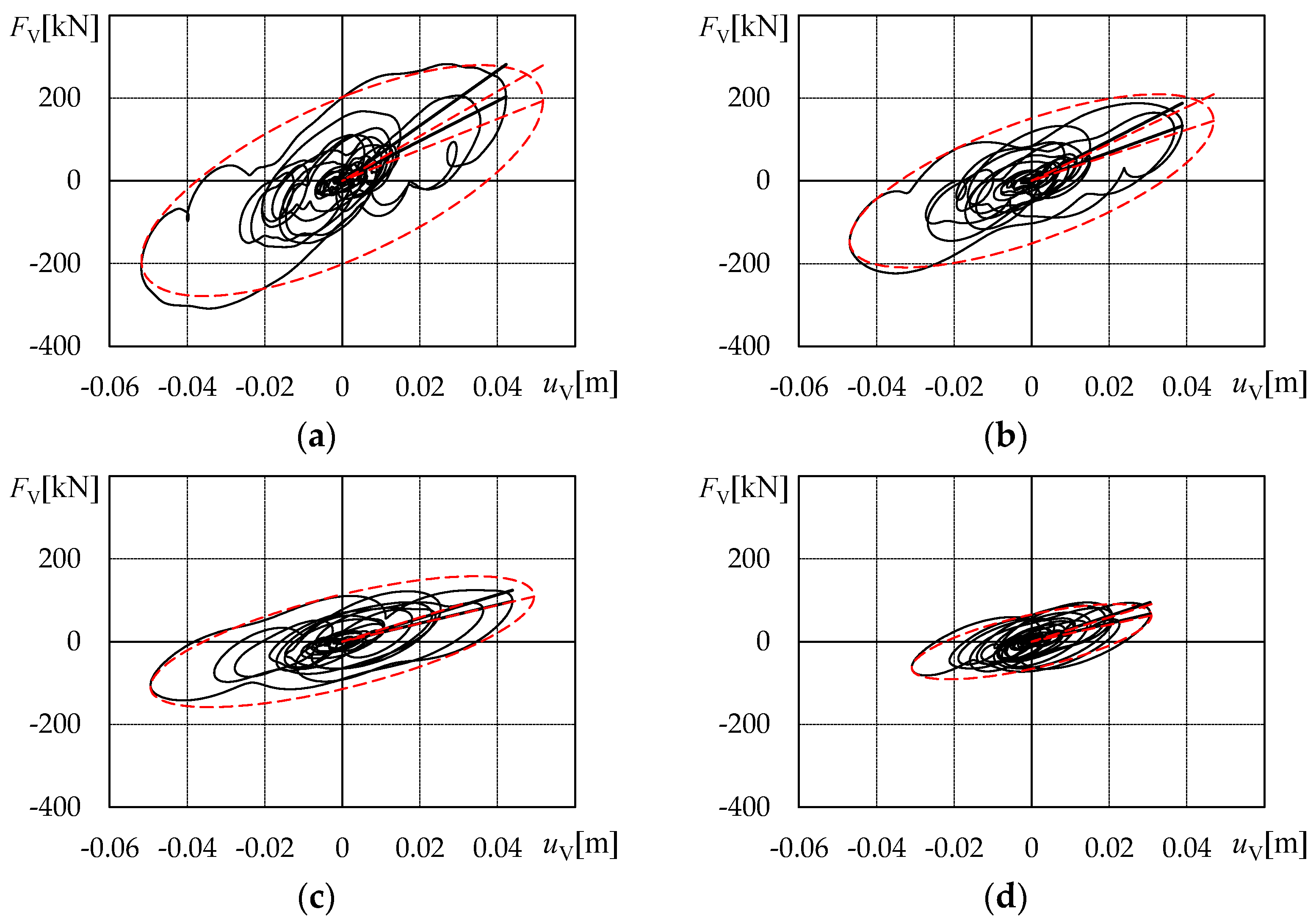
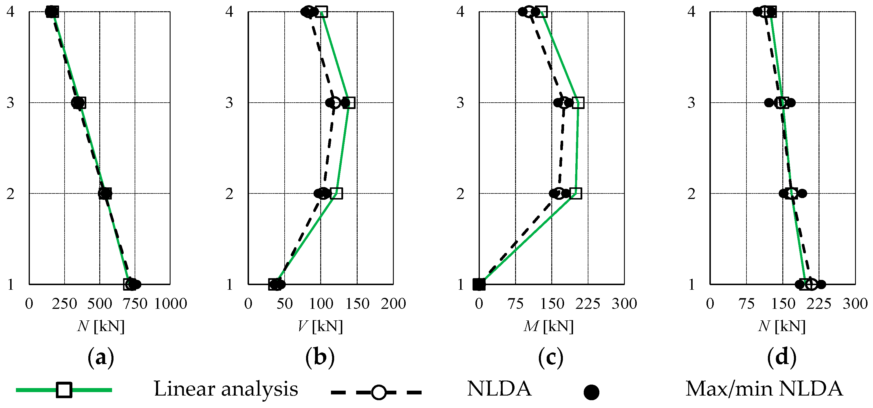
Disclaimer/Publisher’s Note: The statements, opinions and data contained in all publications are solely those of the individual author(s) and contributor(s) and not of MDPI and/or the editor(s). MDPI and/or the editor(s) disclaim responsibility for any injury to people or property resulting from any ideas, methods, instructions or products referred to in the content. |
© 2024 by the authors. Licensee MDPI, Basel, Switzerland. This article is an open access article distributed under the terms and conditions of the Creative Commons Attribution (CC BY) license (https://creativecommons.org/licenses/by/4.0/).