Back to the Metrics: Exploration of Distance Metrics in Anomaly Detection

Abstract

With increasing researched focus on industrial anomaly detection, numerous methods have emerged in this domain. Notably, memory bank-based approaches coupled with k distance metrics have demonstrated remarkable performance in anomaly detection (AD) and anomaly segmentation (AS). However, upon examination of the back to the feature (BTF) method applied to the MVTec-3D AD dataset, it was observed that while it exhibited exceptional segmentation performance, its detection performance was lacking. To address this discrepancy, this study improves the implementation of BTF, especially the improvement of the anomaly score metric. It hypothesizes that when calculating the anomaly score for each sample, only the k-nearest neighbors within the same cluster should be considered. For ease of algorithm implementation, this assumption is distilled into the proposition that AD and AS tasks necessitate different k values in k distance metrics. Consequently, the paper introduces the BTM method, which utilizes distinct distance metrics for AD and AS tasks. This innovative approach yields superior AD and AS performance (I-AUROC 93.0%, AURPO 96.9%, P-AUROC 99.5%), representing a substantial enhancement over the BTF method (I-AUROC 5.7% ↑, AURPO 0.5% ↑, P-AUROC 0.2% ↑).

1. Introduction

Anomaly detection (AD) aims to determine instances that diverge from the “normal” data in the general sense [1,2,3,4]. Meanwhile, anomaly segmentation (AS) looks into specific anomalous instances and precisely delineates the abnormal regions, such as identifying the locations of abnormal pixels. The combined field of anomaly detection and segmentation (AD&S) plays a critical role in various applications, including industrial inspection, security surveillance, and medical image analysis [3,5,6].

1.1. Two-Dimensional Industrial Anomaly Detection

When 2D industrial anomaly detection becomes increasingly emphasized, datasets such as MVTec AD [5,6], BTAD [7], MTD [8], and MVTec LOCO AD [9] are successively introduced. MVTec AD includes various industrial objects and materials with normal and anomalous samples, BTAD focuses on transparent bottle anomalies, MTD targets defects in magnetic tiles, and MVTec LOCOAD evaluates methods under logical constraints and complex scenes. This has stimulated the development of industrial AD&S and facilitated the proposal of many novel AD&S methods. We categorize these methods into three main types:

• Supervised Learning: These algorithms treat anomaly detection as an imbalanced binary classification problem. This approach suffers from the scarcity of abnormal samples and the high cost of labeling. To deal with these problems, various methods have been proposed to generate anomalous samples so as to alleviate the labeling cost. For example, CutPaste [10] and DRAEM [11] manually construct anomalous samples; SimpleNet [12] samples anomalous features near positive sample features; NSA [13] and GRAD [14] synthesize anomalous samples based on normal samples. Despite the diversity of anomaly generation methods, they consistently fail to address the underlying issue of discrepancies between the distributions of generated and real data [15,16,17].
• Unsupervised Learning: These algorithms operate under the assumption that data follow a normal distribution. For example, SROC [18] and SRR [19] rely on this assumption to identify and remove minor anomalies from normal data. When combined with semi-supervised learning techniques, these algorithms achieve enhanced performance.
• Semi-supervised Learning: The concentration assumption, which supposes the normal data are usually bound if the features extracted are good enough, is commonly used when designing semi-supervised learning AD&S methods. These algorithms require only labels for normal data and assume boundaries in the normal data distribution for anomaly detection. Examples include the following: autoencoder-based [20,21,22], GAN-based [20,23,24,25], flow-based [26,27,28,29,30], and SVDD-based methods [31,32,33]. Some memory bank-based methods (MBBM) [16,17,34,35,36,37] that combine pre-trained features from deep neural networks with traditional semi-supervised algorithms have achieved particularly outstanding results and also possess strong interpretability. In rough chronological order, we summarize the main related algorithms as follows:

  (a)

  DN2 [34] was the first to use k-nearest neighbors (kNN) with deep pre-trained features for the AD task, introducing group anomaly detection (GAD) [38]. After that, some works [16,17] fit Gaussian distributions to deep pre-trained features for anomaly scoring using the Mahalanobis distance.

  (b)

  SPADE, building on DN2, [35] employs feature pyramid matching to achieve image AD&S.

  (c)

  PaDiM [36] models pre-train feature patches with Gaussian distributions for better AD&S performance.

  (d)

  Panda [33] sets subtasks based on pre-trained features for model tuning to achieve better feature extraction and improve model performance.

  (e)

  PatchCore [37] and ReConPatch [39] have achieved excellent performance by utilizing downsampled pre-trained feature sets from the kNN method. They have consistently held top positions on the performance leaderboard for an extended period.

1.2. Three-Dimensional Industrial Anomaly Detection

To fill the gap in the 3D AD&S domain, the MVTec-3D AD [40] dataset along with its corresponding baseline algorithms and performance metrics were released to the public, which introduced new opportunities and challenges to industrial AD&S. In subsequent research, various novel methods have been developed and achieved notable results. These include methods based on teacher–student networks such as 3D-ST [41] and AST [42], methods leveraging the PatchCore scoring function like (back to the features) BTF [43] and M3DM [44], and methods focused on constructing anomalies such as 3DSR [45]. Additionally, approaches that utilize neural implicit functions and pre-trained models, exemplified by shape-guided methods [46], have been introduced. These studies primarily aim to design new methods for 3D feature extraction and feature integration.

In the MVTec-3D AD dataset, it was observed that BTF achieved significant performance in terms of AS but lagged in AD performance. Upon further investigation, it was found that methods such as ReConPatch, BTF, and M3DM perform anomaly scoring calculations based on the PatchCore method. These algorithms differ significantly from the initially proposed image domain anomaly scoring algorithm based on kNN [34] and the traditional kNN classification algorithm [47]. The papers lacked specific discussion when introducing these differences. In this paper, the distance measures involved in these algorithms are compared and analyzed, and their advantages and disadvantages are pointed out. According to these advantages and disadvantages, combined with our improvement of the existing MBBM method, we propose a method that uses different anomaly scores in the AD and AS phases, respectively.

1.3. Evaluation Metrics

In this study, we use several key evaluation metrics to assess the performance of our proposed method, including I-AUROC [5,6], P-AUROC [5,6], and AUPRO [6,43,44].

• I-AUROC (instance-based AUROC): This metric measures the AUROC at the instance level, which is crucial for image anomaly detection. It calculates the AUROC value for each image or object, providing an evaluation of the model’s performance on individual instances (detection performance). The formula is as follows:

  $$I-AUROC=\mathrm{AUROC}(y_i,{\widehat{y}}_i),$$

  (1)

  where $y_i$ is the true label of instance i, and ${\widehat{y}}_i$ is the predicted probability for instance i. This metric ranges from 0 to 1. A value closer to 1 indicates better detection performance by the model. A value close to 0.5 suggests that the model is ineffective, and its predictive performance can be considered equivalent to that of a random prediction model.
• P-AUROC (pixel-based AUROC): This metric calculates the AUROC at the pixel level, which is essential for evaluating the performance of anomaly segmentation tasks. It considers the predictions and true labels of each pixel within the images. The formula is as follows:

  $$P-AUROC=\mathrm{AUROC}(y_j,{\widehat{y}}_j),$$

  (2)

  where $y_j$ is the true label of pixel j, and ${\widehat{y}}_j$ is the predicted probability for pixel j. This metric ranges from 0 to 1. A value closer to 1 indicates better segmentation performance by the model. A value close to 0.5 suggests that the model is ineffective, and its predictive performance can be considered equivalent to that of a random prediction model. Due to the special nature of anomaly detection tasks, where normal pixels vastly outnumber abnormal ones, the reference value of this metric for segmentation performance is relatively low.
• PRO (per-region overlap): This metric evaluates the overlap between predicted anomaly regions and ground truth regions, specifically for anomaly segmentation. The formula is as follows:

  $$PRO(T,P)={\displaystyle \frac{1}{K}}\sum _{k=1}^K{\displaystyle \frac{|P\cap T_k|}{|T_k|}},$$

  (3)

  where K is the number of ground truth anomaly regions, P is the set of predicted anomaly regions (multiple connected components), and $T_k$ is the k-th ground truth anomaly region (a single connected component). $|·|$ denotes the number of pixels in a connected component. PRO considers the size and location of anomaly regions, making it useful for evaluating segmentation performance.
• AUPRO (area under the PRO curve): This metric evaluates the performance of anomaly segmentation by calculating the area under the PRO curve. PRO measures the overlap between predicted and ground truth anomaly regions. The formula is as follows:

  $$AUPRO={\int }_0^{1}PRO(T,\mathbb{I}({\widehat{y}}_s>\mathcal{T}))d\mathrm{FPR}$$

  (4)

  where T is the true segmentation label (pixel-level) of a image (a binary matrix, the set of connected pixels with a value of 1 represents a connected component), ${\widehat{y}}_s$ is the set of predicted anomaly scores for each pixel in the image, FPR represents the false positive rate at different thresholds $\mathcal{T}$, and $PRO(T,\mathbb{I}({\widehat{y}}_s>\mathcal{T}))$ is the PRO score at the corresponding threshold $\mathcal{T}$. $\mathcal{T}$ is initialized to the minimum prediction score that makes FPR 0, and as $\mathcal{T}$ decreases, FPR exhibits a discrete upward trend, with the actual integral computed through numerical integration methods. This metric ranges from 0 to 1. A value closer to 1 indicates better segmentation performance by the model. A value close to 0.5 suggests that the model is ineffective, and its predictive performance can be considered equivalent to that of a random prediction model. AUPRO is similar to AUROC but is specifically designed for anomaly segmentation tasks, summarizing the model’s performance across different thresholds.

In the field of industrial anomaly detection, our work primarily focuses on the I-AUROC as the key performance metric, with AUPRO as the secondary metric. For practical applications, especially when emphasizing model performance at lower false positive rates (FPR), we often set an upper limit for AUPRO integration. By choosing 0.3 as the upper limit, we calculate the area under the PRO curve only for FPR between 0% and 30%.

1.4. Contributions and Paper Organization

The key contributions of this work include the following:

• Methodological clarification (PatchCore and BTF): We compare and analyze the theoretical framework and official implementation of PatchCore and BTF. Then, we make improvements to some details found in the paper or code while clarifying the framework of BTM.
• Distance metric analysis: We visualize and analyze the distance measure in the anomaly scoring algorithm, providing initial insights into its strengths and weaknesses. Based on these analyses, we also propose some assumptions.
• Method proposed: On the basis of BTF, a method named back to the metrics (BTM) is proposed in Section 2.1, which achieves the performance improvement of (I-AUROC 5.7% ↑, AURPO 0.5% ↑, and P-AUROC 0.2% ↑). It is also competitive against other leading methods.

This paper is divided into three parts:

• Section 2 optimizes k-nearest neighbor feature fusion, feature alignment, and distance metrics based on BTF and proposes the BTM method. Then, the basis of modification is introduced, including a summary of the framework of MBBM method and an analysis of the implementation details of MBBM (anomaly score calculation, feature fusion, and the downsampling method).
• Section 3 first provides comprehensive information on the datasets used, code implementation details, and parameters used. On this basis, it then compares the performance of the proposed method in Section 2 using real datasets.
• Section 4 summarizes the conclusions drawn in this work and explores future research directions.

2. Methodology

2.1. Back to the Metric

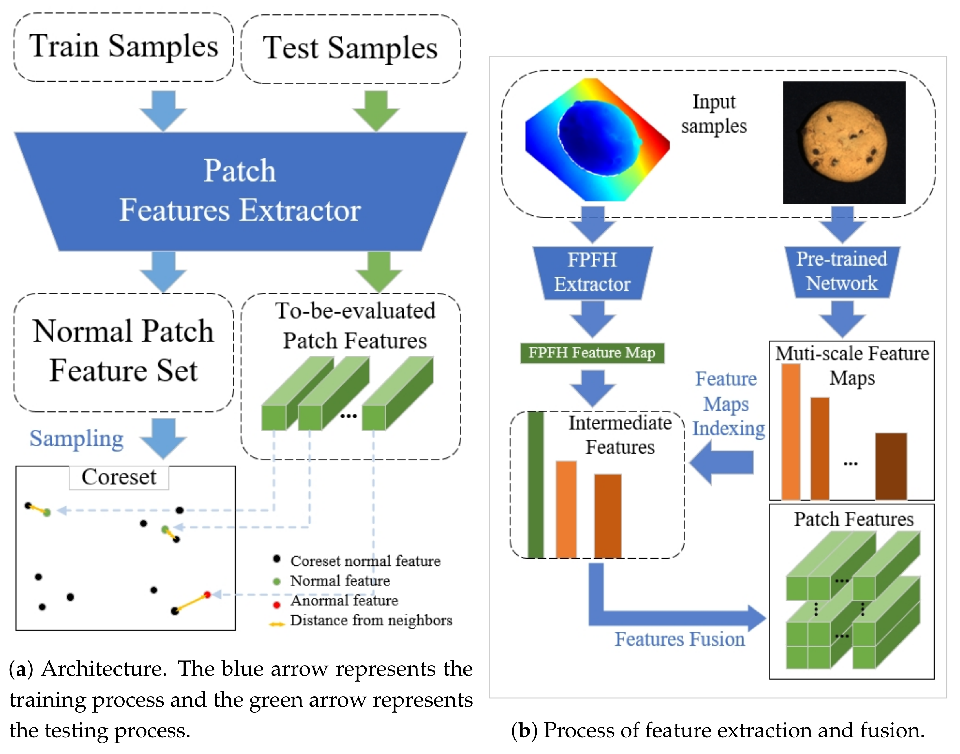
2.1.1. Framework

This section describes the general framework of BTM method through a summary of the MBBM method.

In BTM, we followed the traditional MBBM framework illustrated in Figure 1. Specifically, Figure 1a is dedicated to introducing MBBM. For methods focused solely on anomaly detection (AD), it can be elucidated that the patch features extractor (PFE) extracts only one feature for each sample. In other words, such methods treat the entire image as a single patch. Figure 1b shows the feature extraction process of the BTM method on the MVTec-3D AD dataset. The process depicted is consistent with BTF, with variations noted in Section 2.1.2 and Section 3.3.

2.1.2. Optimization

On the framework shown in Figure 1, we opt to use kNN squared distance mean metrics as the anomaly score calculation function for AS tasks, and employ nearest neighbor metrics to compute image-level anomaly scores. We term this approach BTM and conduct AD&S experiments on the MVTec-3D AD dataset.

Building upon BTF, we reference DN2’s work on GAD and, considering the alignment requirements between images and features, utilize a mean convolution kernel with kernel-size = 3, stride = 1, and padding = 1 to fuse neighboring features. For the sake of logical correctness and code parallelism, we replace the elliptical Gaussian blur kernel used in computing AS anomaly scores with a Gaussian blur kernel of kernel-size = 15 and sigma = (4, 4), directly applicable to tensors. We will get into the details of why these changes were made in a later section.

2.2. The Structure of Memory Bank-Based Methods (MBBM)

2.2.1. Anomaly Score Metrics

Traditional kNN algorithm is a classification algorithm based on similarity metrics. It determines the category of a new sample by selecting kNN to vote, where k is usually chosen as an odd number to avoid ties during the voting process [47]. In semi-supervised anomaly detection, anomalous samples do not appear in the training set. In contrast, the MBBM considers the influence of multiple different normal samples in the anomaly scoring function through techniques like re-weighting.

DN2 is the first model to introduce a kNN-based method in industrial image anomaly detection, scoring image anomalies using Equation (5).

$$s=d\left(x\right)={\displaystyle \frac{1}{k}}\sum _{f\in {\mathcal{N}}_k\left(f_x\right)}{\parallel f-f_x\parallel }_2.$$

(5)

The symbol ${\mathcal{N}}_k\left(f_x\right)$ represents the set of k-nearest feature vectors to $f_x$ within the training set $F_{\mathrm{train}}$. The anomaly score s of the test image is denoted by the distance function $d\left(x\right)$, which is the average sum of squared Euclidean distances between the feature vector $f_x$ and the feature vectors f in its kNN ${\mathcal{N}}_k\left(f_x\right)$. The rule with $k=1$ is commonly referred to as the nearest neighbor rule [47].

Work such as SPADE further extends DN2 to AS tasks. For an image sample that is divided into I rows and J columns, $f_{i,j}$ represents the feature extracted from the patch at the ith row and jth column, and

$$F=\{f_{i,j}\mid 0\le i<I,0\le j<J\}$$

represents the set of features for the entire image. Let $s_{i,j}$ represent the anomaly score of the patch at the ith row and jth column. Let $\mathcal{M}$ represent the coreset of features obtained by applying a greedy algorithm for subsampling on the set of patch features from all images in the training set. Let ${\mathcal{N}}_k\left(f_y\right)$ represent the set of k nearest features to $f_y$ in $\mathcal{M}$.

$$s_{i,j}={\displaystyle \frac{1}{k}}\sum _{f\in {\mathcal{N}}_k\left(f_{i,j}\right)}{\parallel f-f_{i,j}\parallel }_2.$$

(6)

For each image, PatchCore’s official code uses Equation (6) for AS anomaly score calculation, where $k=1$ in the paper, which can be represented by Equation (7).

$$s_{i,j}=\underset{m\in \mathcal{M}}{min}{\parallel m-f_{i,j}\parallel }_2.$$

(7)

PatchCore defines the maximum distance score $s^{*}$ of a test image, which can be expressed as Equation (8) or more closely to the original text as Appendix A (less rigorous). Here, $f_{i^{*},j^{*}}$ is the feature in the test image with the highest anomaly score, and $m^{*}$ is the feature in the core set $\mathcal{M}$ that is nearest to $f_{i^{*},j^{*}}$.

$$s^{*}=\underset{0\le i<I,0\le j<J}{max}{s}_{i,j}.$$

(8)

It is noteworthy that, in conjunction with the understanding of Equations (7) and (8), we propose that the terms $m^{*}$ and $f_{i^{*},j^{*}}$ in Equations (A1) and (A2) need to be redefined, as shown in Equation (9). Here, $m_{i,j}$ represents the nearest neighbor of $f_{i^{*},j^{*}}$ within $\mathcal{M}$, and $S_{fm}$ denotes the set composed of tuples, each consisting of all patch features from an image and their respective nearest neighbors in $\mathcal{M}$.

$$\begin{array}{cc}\hfill m_{i,j}& =\underset{m\in \mathcal{M}}{\arg \min }{\parallel m-f_{i,j}\parallel }_2,\hfill \\ \hfill S_{fm}& =\{(f_{i,j},m_{i,j})\mid 0\le i<I,0\le j<J\},\hfill \\ \hfill (f_{i^{*},j^{*}},m^{*})& =\underset{(f_{i,j},m_{i,j})\in S_{fm}}{\arg \max }{\parallel m_{i,j}-f_{i,j}\parallel }_2,\hfill \end{array}$$

(9)

$$w=\left(1-{\displaystyle \frac{exp\left({\parallel f_{i^{*},j^{*}}-m^{*}\parallel }_2\right)}{{\sum }_{m\in {\mathcal{N}}_k\left(m^{*}\right)}exp\left({\parallel f_{i^{*},j^{*}}-m\parallel }_2\right)}}\right),$$

(10)

$$s=w·s^{*}.$$

(11)

To make the image anomaly scoring results more robust [37], PatchCore employs the weights w from Equation (10) to reweight $s^{*}$ as the anomaly score, as shown in Equation (11). BTF and M3DM both implement Equation (10) in their code but M3DM employs complex methods such as reweighting and one-class support vector machines for anomaly score re-calculation.

$$\begin{array}{cc}\hfill {\alpha }_1& ={\displaystyle \frac{exp\left({\parallel f_{i^{*},j^{*}}-m^{*}\parallel }_2\right)}{{{\displaystyle \sum }}_{m\in {\mathcal{N}}_k\left(m^{*}\right)}exp\left({\parallel f_{i^{*},j^{*}}-m\parallel }_2\right)}},\hfill \\ \hfill {\alpha }_2& ={\displaystyle \sum }_{m\in {\mathcal{N}}_k\left(m^{*}\right)}exp\left({\parallel f_{i^{*},j^{*}}-m\parallel }_2\right),\hfill \\ \hfill & ={\displaystyle \sum }_{m\in {\mathcal{N}}_k\left(m^{*}\right)}exp\left(\sqrt{f_{i^{*},j^{*}}^T{f}_{i^{*},j^{*}}-2f_{i^{*},j^{*}}^{T}m+m^{T}m}\right),\hfill \\ \hfill & ={\displaystyle \sum }_{m\in {\mathcal{N}}_k\left(m^{*}\right)}exp\left(\sqrt{{\parallel f_{i^{*},j^{*}}\parallel }_2^2-2f_{i^{*},j^{*}}^{T}m+{\parallel m\parallel }_2^2}\right).\hfill \end{array}$$

(12)

To facilitate further analysis, we define partial component factors (or terms) ${\alpha }_1$ and ${\alpha }_2$ of the variable w, as shown in Equation (12). The exponential function $exp(·)$ and the square root function $\sqrt{·}$ are monotonically increasing and, therefore, not specifically considered.

In the analysis of ${\alpha }_2$, the terms ${\parallel f_{i^{*},j^{*}}\parallel }_2^2$, ${\parallel m\parallel }_2^2$, and $f_{i^{*},j^{*}}^{T}m$ can have adverse effects on the contour plots of the anomaly scores. These factors can lead to distortions in the visualization, making it challenging to accurately interpret the results. The impact of these terms on the anomaly contour plots is illustrated in Section 2.3.1.

In summary, the officially released PatchCore-derived methods currently primarily utilize the anomaly score Equations (6) and (7) for the AS task, and Equations (6), (7), and (9) for the AD task.

2.2.2. Feature Fusion

In pure image anomaly detection (AD) tasks, the issue of feature fusion is not inherently involved. However, DN2 is explored as a GAD problem: as shown in Figure 2, DN2 compares three methods of feature fusion, concatenate, max, and mean, and found that using the mean for feature fusion combined with the kNN anomaly score calculation algorithm resulted in the best ROCAUC performance. In contrast, the performance of the concatenate method in terms of ROCAUC first increased and then decreased with the enlargement of the group size. This experiment offers some inspiration for feature fusion methods in subsequent work.

In the anomaly score (AS) of methods derived from PatchCore, two variants of feature fusion appear: (1) on the MVTec-3D AD dataset, the PatchCore code upsamples the high-level feature map to the same resolution as the low-level features using bilinear interpolation, then maps different levels to the same dimension (e.g., hyperparameter 1024), concatenates them together, and finally maps them to a feature vector of a specific dimension. (2) On 3D datasets, BTF and M3DM first use the mean method to perform domain feature fusion for different layer features (including RBB multi-scale features and geometric features), then the high-level feature map is upsampled to the same resolution as the low-level features using bilinear interpolation, and finally, the features from all layers are concatenated together to generate a feature vector.

Overall, the fusion of features from the same modality, such as the fusion of features from the same spatial domain, can be approached as a GAD problem, where using the mean method can yield better performance, especially when many features are involved. On the other hand, for the fusion of features from different modalities, including different scales and different characteristics, concatenation is a more common choice. More sophisticated and complex feature fusion techniques, such as those used by M3DM, are beyond the scope of this discussion.

Referring to DN2’s work on GAD, in BTM we make the mean convolution kernel of size 3 and step 1 perform neighbor feature fusion, which is the same as in BTF. The difference is, given the feature alignment, we add padding of size 1 to the convolution kernel. For features other than nearest neighbor features, we simply use concatenate as a feature fusion method.

2.2.3. The Iterative Greedy Approximation Algorithm

Both PatchCore and BTF utilize the iterative greedy approximation (IGA) algorithm [48] to subsample the memory bank. IGA significantly addresses the issue of overemphasis on outlier samples in both active learning and anomaly detection scenarios. This method ensures the coverage, representativeness, and information complexity of the coreset samples. However, it is worth noting that in active learning, the normalcy of outliers is not a primary concern, whereas in anomaly detection, it is important.

The IGA algorithm tends to collect samples at the edges of sample clusters, typically high-frequency samples around low-frequency regions. Based on this characteristic of the IGA algorithm, we have the following assumptions:

Assumption 1.

If there are abnormal samples in the training set, they are likely to be captured by IGA and become outliers (considered normal) in the core set.

Assumption 2.

In low-frequency areas near high-frequency features (the boundary of the sample cluster), data points are likely to be outliers and should receive higher anomaly scores.

2.3. Visualization Analysis of Different Metrics

In MBBM, the interaction between the anomaly score calculation function and feature engineering ultimately affects the calculation of anomaly scores. In existing research on image anomaly detection, the evaluation of anomaly score calculation functions is typically manifested as performance metrics on specific datasets. However, this is far from sufficient [49]. Considering the inherent flaws of real datasets and the significant impact of complex variable interactions on results, we simulate sample distributions in two-dimensional space to facilitate the visual analysis of anomaly score functions.

$$\begin{array}{cc}\hfill v_x& =\left\{x\in \mathbb{R}\mid x=x_0+0.005n,n\in \mathbb{N},0\le n<{\displaystyle \frac{x_1-x_0}{0.005}}\right\},\hfill \\ \hfill v_y& =\left\{y\in \mathbb{R}\mid x=y_0+0.005n,n\in \mathbb{N},0\le n<{\displaystyle \frac{y_1-y_0}{0.005}}\right\},\hfill \\ \hfill Grid& =v\times v,\mathrm{where}Grid\in {\mathbb{R}}^{\lfloor (x_1-x_0)(y_1-y_0)\rfloor /0.00005\times 2}.\hfill \end{array}$$

(13)

As shown in Equation (13), this study uses $v_x$ and $v_y$ to denote one-dimensional grid vectors along the x and y axes within the visualization region ($x_0<x<x_1,y_0<y<y_1$) and employs $Grid$ to represent the two-dimensional spatial vector for visualization. The values $x_0$, $x_1$, $y_0$, and $y_1$ are manually input to define the visualization range. We employ random sampling within the grid to generate a core set $\in {\mathbb{R}}^{n\times 2}$, and subsequently, visualize the gradient of anomaly scores within the $Grid$ range.

The set $dists=\left\{(\parallel x-c{\parallel }_2)\mid x\in Grid,c\in coreset\right\}$ denotes the Euclidean distance between the points $(x,y)$ in $Grid$ and points c in $coreset$. By substituting $dists$ into the corresponding formula, one can obtain the anomaly score or anomaly score weights Z, which are ultimately used to draw contours. Both $dists$ and the anomaly scores can be obtained through parallel computation.

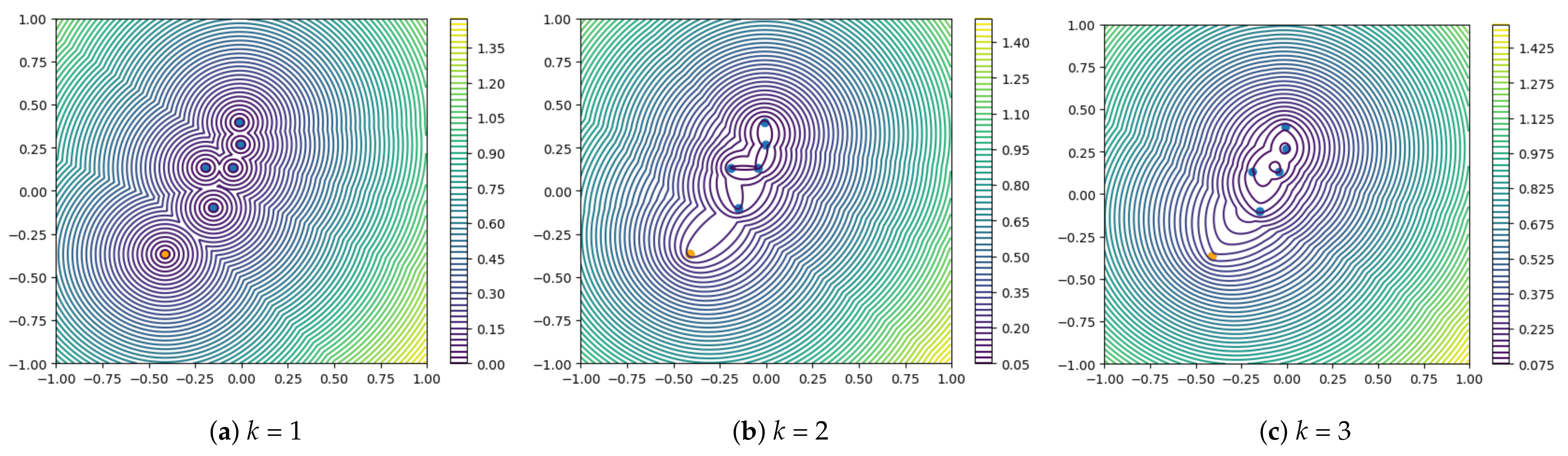
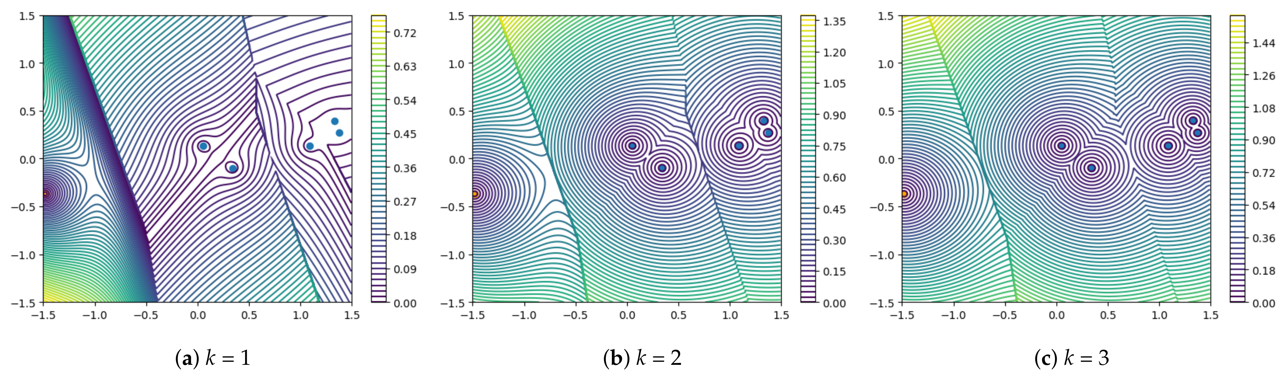
2.3.1. k-Nearest Neighbor Squared Distance Mean

When $k=1$, as shown in Figure 3a, the algorithm ensures adequate sample coverage and representativeness. As k increases, as illustrated in Figure 3, the coverage and representativeness of outlier points significantly decrease while the robustness of the anomaly score calculation function to outlier points slightly improves.

Larger k values can increase the robustness of the model and reduce the influence of outliers but at the expense of sample representativeness and coverage. When k > 1, we see a score distribution that conforms to Assumption 2. When the number of test samples is large enough and most of them are normal, it is a good choice to increase the k value appropriately to increase the robustness of the abnormal samples that may be introduced by Assumption 1. This fits the scenario of the AS task.

However, as we can see from Figure 3b, when k increases, there will be many “gullies” in the gradient plot of the abnormal fraction function. These “gullies” exist regardless of whether the outliers are normal or abnormal. Samples located in gullies will be assigned the same anomaly scores, losing their ability to distinguish anomalies. During patch core and BTF process AD tasks, the patch with the highest anomaly score plays a decisive role. In cases where a known sample is likely to be an anomaly (has a high probability of not being affected by outliers and reducing the anomaly score), the presence of these gullies is not conducive to the recall of anomalies.

To sum up, MBBM uses the k-nearest neighbor squared distance mean to measure the k value that may be needed for processing AS tasks. It is best to maintain k = 1 when processing AD tasks.

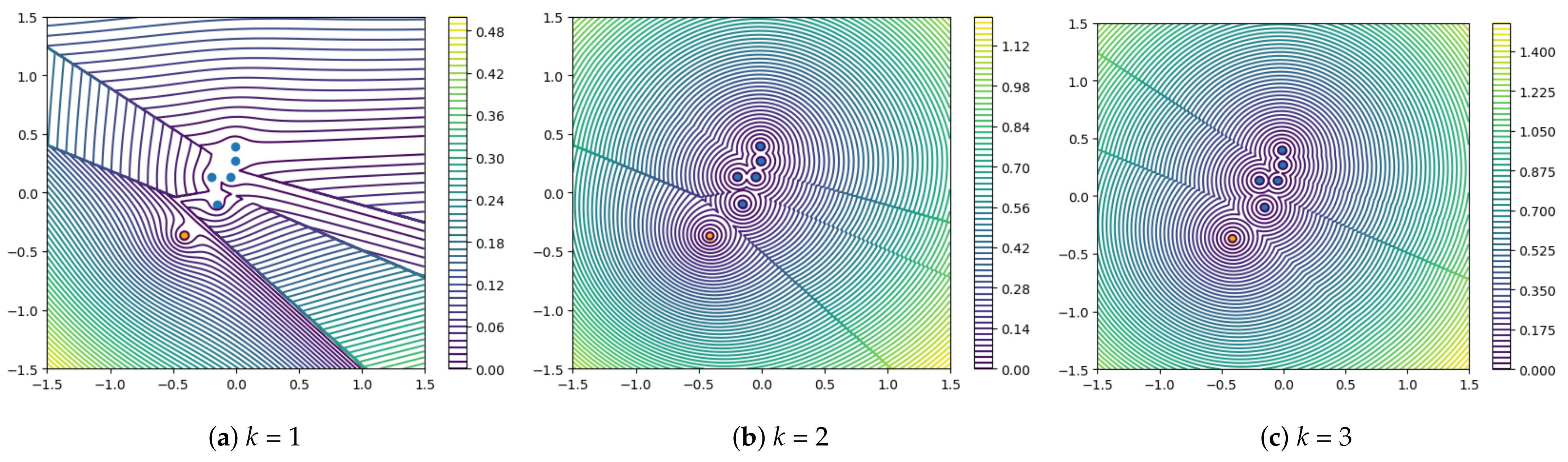
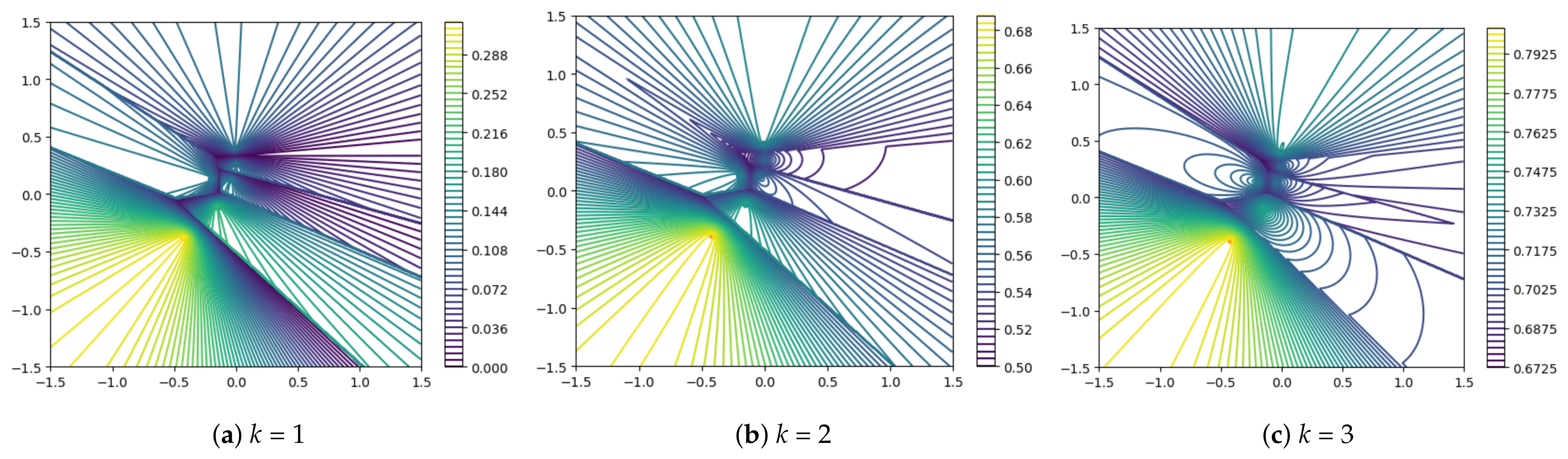
2.3.2. PatchCore Anomaly Score Calculation Function

The function composition of ${\alpha }_1$ resembles Softmax. As shown in Figure 4, ${\alpha }_1$ has larger values at the boundaries of the sample coverage area. As k increases, the maximum value of ${\alpha }_1$ first decreases rapidly and then decreases slowly, approximately inversely proportional to k. Combining Equations (11) and (12), we can observe that as k increases, the weight w tends to approach 1, and the influence of distance variance on the final anomaly score decreases.

Figure 5 and Figure 6 illustrate the behavior of s and w in Equation (11). w increases with the increase of k, while its factor ${\alpha }_1$ decreases significantly. Except for Figure 5a, which exhibits a bizarre distribution of anomalies due to excessive influence from ${\alpha }_1$, assuming a randomly distributed sample set, both Figure 5b and Figure 5c are relatively reasonable: they conform to Assumption 2. If the outliers in the normal samples are marginal samples of this cluster, the gradient of anomaly scores on the outlier side is larger.

In other words, w induces a subtle merging phenomenon in the distribution of anomaly scores for the k nearest neighbors of each point. This has adverse effects on the distribution of anomaly scores for clusters with a size less than or equal to k.

As shown in Figure 7b, when $k=2$, the distribution of anomaly scores around the cluster composed of three sample points on the right side of the image does not exhibit significant inward shifting, forming a closed whole. Around the cluster composed of two sample points in the middle, a slight phenomenon of shifting towards the right side appears. While around the cluster composed of one sample point on the left side, there is a clear tendency for merging towards the right side. All clusters shown in Figure 7b exhibit slight merging phenomena. These merging or shifting phenomena are inconsistent with our assumptions.

2.3.3. Summary

In summary, the k-nearest neighbor squared distance mean score calculation function has obvious drawbacks when $k>1$, but it exhibits better universality when $k=1$. In most cases, particularly when it is highly probable that the sample is anomalous (anomaly detection tasks generally use the highest anomaly score sample from anomaly segmentation for further anomaly score calculation), this method does not produce the extreme errors seen in previous re-weighting methods. The PatchCore anomaly score calculation function can have better distribution patterns of anomaly scores in certain situations, but it imposes stringent requirements on the sampling method and the distribution of sampling results. When using the kNN distance metric to calculate the anomaly score, k needs to be smaller than the number of samples in the cluster, and the anomaly detection performance is best when k is close to the number of samples in the cluster. Accounting for the above visual analysis results, as shown in Equation (14), we define the memory bank ${\mathcal{M}}^{\prime }$ as a set consisting of many clusters $\mathcal{C}$, each of which consists of kNN samples. In the equation, d should be defined based on empirical observations. Choosing a suitable k for each cluster in the anomaly scoring phase is noteworthy. However, for computational and implementation convenience, we simply assume that the k values of $\mathcal{C}$ in ${\mathcal{M}}^{\prime }$ close to the abnormal samples of the test set are small, while the k values of other $\mathcal{C}$ are large.

$$\begin{array}{cc}\hfill {\mathcal{M}}^{\prime }& =\{\hfill \\ \hfill & {\mathcal{C}}_1,{\mathcal{C}}_2,\dots ,{\mathcal{C}}_n|n\in {\mathbb{Z}}^{+},\hfill \\ \hfill & (\forall c\in {\mathcal{C}}_n,\exists c^{\prime }\in {\mathcal{C}}_n\setminus \left\{c\right\},\mathrm{dist}(c,c^{\prime })\le d),\hfill \\ \hfill & (\forall c\in {\mathcal{C}}_n,\forall c^{\prime }\in \mathcal{M}\setminus {\mathcal{C}}_n,\mathrm{dist}(c,c^{\prime })>d)\hfill \\ \hfill & \},\hfill \\ \hfill \mathcal{M}& =\bigcup _{\mathcal{C}\in {\mathcal{M}}^{\prime }}\mathcal{C}.\hfill \end{array}$$

(14)

We pay more attention to abnormal samples in the anomaly detection (AD) task, while normal samples are more predominant in the anomaly scoring (AS) task. Therefore, we should set different values of k for anomaly score calculation in AD and AS. Specifically, a smaller k value is designed for AD anomaly score calculation, and a larger k value is designed for AS anomaly score calculation.

3. Experiments

3.1. Datasets

The MVTec AD dataset is a comprehensive benchmark dataset for evaluating anomaly detection algorithms in industrial inspection scenarios. It consists of over 5000 high-resolution color images across 15 different object and texture categories. The dataset includes both normal images for training and validation, as well as anomalous images for testing, with various types of real-world defects such as scratches, dents, and contaminations. The objects and textures in the dataset exhibit a range of complexities and challenges for anomaly detection, making it a valuable resource for developing and assessing the performance of unsupervised and semi-supervised anomaly detection methods in the context of manufacturing and quality control [5,6].

The MVTec-3D AD dataset comprises 4147 high-resolution industrial 3D scans across 10 object categories. It includes anomaly-free scans for training and validation, as well as test samples with various real-world anomalies like scratches, dents, and contaminations. The objects range from those with natural variations (bagel, carrot, cookie, peach, and potato) to standardized but deformable ones (foam, rope, and tire) and rigid ones (cable gland, and dowel). The dataset is designed for unsupervised anomaly detection in industrial inspection scenarios, featuring 41 types of anomalies [40].

3.2. Evaluation Metrics

This work compares I-AUROC [5,6] and P-AUROC [5,6] performance with PatchCore (amazon-science/patchcore-inspection; branch:main; commit: fcaa92f124fb1ad74a7 acf56726decd4b27cbcad) on the MVTec AD dataset, and with BTF and M3dM on the MVTec-3D AD dataset with the P-AUROC (integration upper limit set to 0.3) [6,43,44].

3.3. Implementation Details

Our experiments were primarily conducted on the official GitHub repositories of PatchCore and BTF. Except for experimental variables and specifically mentioned parameters, all other parameters remained the same as the official defaults. Even during the performance comparison process, we abandoned many performance optimization techniques, with significant potential performance improvements.

When comparing the performance of AD&S on the MVTec-3D AD dataset using the BTM method with other approaches, we employed the parameter $k=3$, as recommended in the PatchCore paper for the AS task in kNN squared distance mean metrics.

3.4. Performance Comparison

3.4.1. Anomaly Detection on MVTec-3D AD

To compare the anomaly detection (AD) performance, we evaluated BTM against several 3D, RGB, and RGB + 3D multimodal methods on the MVTec-3D dataset. As shown in

Table 1. I-AUROC score for anomaly detection of all categories of MVTec-3D AD. Our method clearly outperforms other methods in the 3D + RGB setting and obtains a 0.930 mean I-AUROC score.

	Method	Bagel	Cable Gland	Carrot	Cookie	Dowel	Foam	Peach	Potato	Rope	Tire	Mean
3D	Depth GAN [40]	0.538	0.372	0.580	0.603	0.430	0.534	0.642	0.601	0.443	0.577	0.532
	Depth AE [40]	0.648	0.502	0.650	0.488	0.805	0.522	0.712	0.529	0.540	0.552	0.595
	Depth VM [40]	0.513	0.551	0.477	0.581	0.617	0.716	0.450	0.421	0.598	0.623	0.555
	Voxel GAN [40]	0.680	0.324	0.565	0.399	0.497	0.482	0.566	0.579	0.601	0.482	0.517
	Voxel AE [40]	0.510	0.540	0.384	0.693	0.446	0.632	0.550	0.494	0.721	0.413	0.538
	Voxel VM [40]	0.553	0.772	0.484	0.701	0.751	0.578	0.480	0.466	0.689	0.611	0.609
	3D-ST	0.862	0.484	0.832	0.894	0.848	0.663	0.763	0.687	0.958	0.486	0.748
	M3DM [44]	0.941	0.651	0.965	0.969	0.905	0.760	0.880	0.974	0.926	0.765	0.874
	FPFH (BTF) [43]	0.820	0.533	0.877	0.769	0.718	0.574	0.774	0.895	0.990	0.582	0.753
	FPFH (BTM)	0.939	0.553	0.916	0.844	0.823	0.588	0.718	0.928	0.976	0.633	0.792
RGB	PatchCore [44]	0.876	0.880	0.791	0.682	0.912	0.701	0.695	0.618	0.841	0.702	0.770
	M3DM [44]	0.944	0.918	0.896	0.749	0.959	0.767	0.919	0.648	0.938	0.767	0.850
	RGB iNet (BTF) [43]	0.854	0.840	0.824	0.687	0.974	0.716	0.713	0.593	0.920	0.724	0.785
	RGB iNet (BTM)	0.909	0.895	0.838	0.745	0.975	0.714	0.79	0.605	0.93	0.759	0.816
RGB+3D	Depth GAN [40]	0.530	0.376	0.607	0.603	0.497	0.484	0.595	0.489	0.536	0.521	0.523
	Depth AE [40]	0.468	0.731	0.497	0.673	0.534	0.417	0.485	0.549	0.564	0.546	0.546
	Depth VM [40]	0.510	0.542	0.469	0.576	0.609	0.699	0.450	0.419	0.668	0.520	0.546
	Voxel GAN [40]	0.383	0.623	0.474	0.639	0.564	0.409	0.617	0.427	0.663	0.577	0.537
	Voxel AE [40]	0.693	0.425	0.515	0.790	0.494	0.558	0.537	0.484	0.639	0.583	0.571
	Voxel VM [40]	0.750	0.747	0.613	0.738	0.823	0.693	0.679	0.652	0.609	0.690	0.699
	M3DM *	0.998	0.894	0.96	0.963	0.954	0.901	0.958	0.868	0.962	0.797	0.926
	BTF [43]	0.938	0.765	0.972	0.888	0.960	0.664	0.904	0.929	0.982	0.726	0.873
	BTM	0.980	0.860	0.980	0.963	0.978	0.726	0.958	0.953	0.980	0.926	0.930

* Denotes results obtained by employing pre-trained parameters provided by the original studies. Unannotated results are directly excerpted from the corresponding literature. The bold method is the method proposed by this paper. The bold number represents the best performance metric in the current modality and category.

, under the RGB + 3D multimodal setting, BTM exhibited an average AD performance improvement of 5.7% compared to the previous BTF method; this advantage was also observed in each individual category. In the RGB and 3D modalities, BTM achieved average performance improvements of 3.1% and 3.9%, respectively, over BTF; again, this improvement was consistent across each category.

We also replicated M3DM using the code and corresponding model parameters from the official GitHub repository. In comparing our results with the replication, our method demonstrated strong competitiveness overall. Specifically, in the RGB + 3D multimodal setting, BTM outperformed M3DM by 0.4%, achieving a performance of 93%. It is worth noting that unlike M3DM, we did not use manually designed foreground templates, leaving significant room for further AD performance enhancement. We prefer to validate the model by preserving the foreground and background to ensure its robustness.

3.4.2. Anomaly Segmentation on MVTec-3D AD

To compare the anomaly scoring (AS) performance, we evaluated BTM against several 3D, RGB, and RGB + 3D multimodal methods on the MVTec-3D dataset. As shown in Table 2, under the RGB + 3D multimodal setting, BTM achieved an average AUPRO performance of 96.9%, surpassing M3DM and BTF by 0.8% and 0.5%, respectively. This superiority was also evident when examining individual categories. In the RGB and 3D modalities, BTM outperformed BTF. It also shows strong competitiveness compared to other methods.

On the MVTec-3D dataset, BTM achieved an average P-AUROC performance of 99.5%, surpassing BTF and M3DM by 0.5% and 0.2%, respectively. Detailed P-AUROC performance comparisons are provided in Table 3.

Similarly, as we did not utilize manually designed foreground templates like M3DM or 3D-ST, we believe there is substantial room for AS performance improvement.

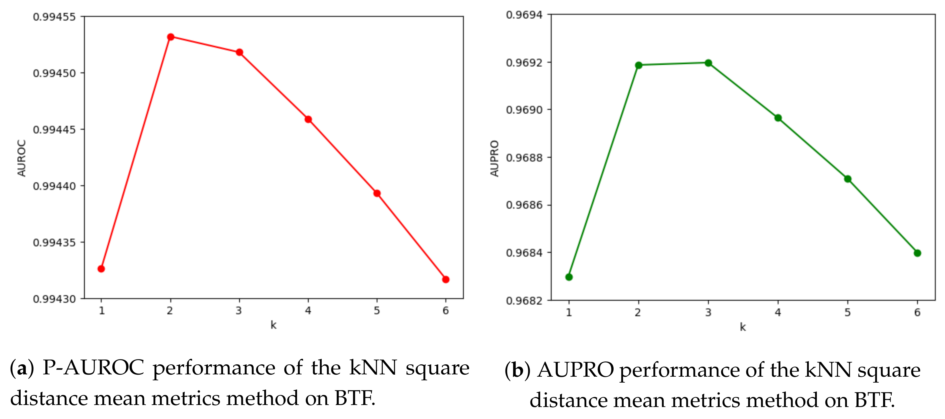
3.5. Performance of kNN Reweight Metrics on BTF

We conducted experiments on computing AD anomaly scores using BTF with a kNN re-weighting approach (Equation 11) on the MVTec-3D AD dataset. As shown in Figure 8, the AD performance is lowest when k = 1. Subsequently, as k increases, the influence of weight w decreases, and the AD performance gradually approaches our optimal performance.

Table 2. AUPRO score for anomaly detection of all categories of MVTec-3D AD. Our method outperforms other methods in the 3D + RGB setting and obtains 0.969 mean AUPRO score.

	Method	Bagel	Cable Gland	Carrot	Cookie	Dowel	Foam	Peach	Potato	Rope	Tire	Mean
3D	Depth GAN [40]	0.111	0.072	0.212	0.174	0.160	0.128	0.003	0.042	0.446	0.075	0.143
	Depth AE [40]	0.147	0.069	0.293	0.217	0.207	0.181	0.164	0.066	0.545	0.142	0.203
	Depth VM [40]	0.280	0.374	0.243	0.526	0.485	0.314	0.199	0.388	0.543	0.385	0.374
	Voxel GAN [40]	0.440	0.453	0.875	0.755	0.782	0.378	0.392	0.639	0.775	0.389	0.583
	Voxel AE [40]	0.260	0.341	0.581	0.351	0.502	0.234	0.351	0.658	0.015	0.185	0.348
	Voxel VM [40]	0.453	0.343	0.521	0.697	0.680	0.284	0.349	0.634	0.616	0.346	0.492
	3D-ST [41]	0.950	0.483	0.986	0.921	0.905	0.632	0.945	0.988	0.976	0.542	0.833
	M3DM [44]	0.943	0.818	0.977	0.882	0.881	0.743	0.958	0.974	0.95	0.929	0.906
	FPFH (BTF) [43]	0.972	0.849	0.981	0.939	0.963	0.693	0.975	0.981	0.980	0.949	0.928
	FPFH (BTM)	0.974	0.861	0.981	0.937	0.959	0.661	0.978	0.983	0.98	0.947	0.926
RGB	PatchCore [44]	0.901	0.949	0.928	0.877	0.892	0.563	0.904	0.932	0.908	0.906	0.876
	M3DM [44]	0.952	0.972	0.973	0.891	0.932	0.843	0.97	0.956	0.968	0.966	0.942
	RGB iNet (BTF) [43]	0.898	0.948	0.927	0.872	0.927	0.555	0.902	0.931	0.903	0.899	0.876
	RGB iNet (BTM)	0.901	0.958	0.942	0.905	0.951	0.615	0.906	0.938	0.927	0.916	0.896
RGB+3D	Depth GAN [40]	0.421	0.422	0.778	0.696	0.494	0.252	0.285	0.362	0.402	0.631	0.474
	Depth AE [40]	0.432	0.158	0.808	0.491	0.841	0.406	0.262	0.216	0.716	0.478	0.481
	Depth VM [40]	0.388	0.321	0.194	0.570	0.408	0.282	0.244	0.349	0.268	0.331	0.335
	Voxel GAN [40]	0.664	0.620	0.766	0.740	0.783	0.332	0.582	0.790	0.633	0.483	0.639
	Voxel AE [40]	0.467	0.750	0.808	0.550	0.765	0.473	0.721	0.918	0.019	0.170	0.564
	Voxel VM [40]	0.510	0.331	0.413	0.715	0.680	0.279	0.300	0.507	0.611	0.366	0.471
	M3DM *	0.966	0.971	0.978	0.949	0.941	0.92	0.977	0.967	0.971	0.973	0.961
	BTF [43]	0.976	0.967	0.979	0.974	0.971	0.884	0.976	0.981	0.959	0.971	0.964
	BTM	0.979	0.972	0.980	0.976	0.977	0.905	0.978	0.982	0.968	0.975	0.969

* Denotes results obtained by employing pre-trained parameters provided by the original studies. Unannotated results are directly excerpted from the corresponding literature. The bold method is the method proposed by this paper. The bold number represents the best performance metric in the current modality and category.

Table 2. AUPRO score for anomaly detection of all categories of MVTec-3D AD. Our method outperforms other methods in the 3D + RGB setting and obtains 0.969 mean AUPRO score.

	Method	Bagel	Cable Gland	Carrot	Cookie	Dowel	Foam	Peach	Potato	Rope	Tire	Mean
3D	Depth GAN [40]	0.111	0.072	0.212	0.174	0.160	0.128	0.003	0.042	0.446	0.075	0.143
	Depth AE [40]	0.147	0.069	0.293	0.217	0.207	0.181	0.164	0.066	0.545	0.142	0.203
	Depth VM [40]	0.280	0.374	0.243	0.526	0.485	0.314	0.199	0.388	0.543	0.385	0.374
	Voxel GAN [40]	0.440	0.453	0.875	0.755	0.782	0.378	0.392	0.639	0.775	0.389	0.583
	Voxel AE [40]	0.260	0.341	0.581	0.351	0.502	0.234	0.351	0.658	0.015	0.185	0.348
	Voxel VM [40]	0.453	0.343	0.521	0.697	0.680	0.284	0.349	0.634	0.616	0.346	0.492
	3D-ST [41]	0.950	0.483	0.986	0.921	0.905	0.632	0.945	0.988	0.976	0.542	0.833
	M3DM [44]	0.943	0.818	0.977	0.882	0.881	0.743	0.958	0.974	0.95	0.929	0.906
	FPFH (BTF) [43]	0.972	0.849	0.981	0.939	0.963	0.693	0.975	0.981	0.980	0.949	0.928
	FPFH (BTM)	0.974	0.861	0.981	0.937	0.959	0.661	0.978	0.983	0.98	0.947	0.926
RGB	PatchCore [44]	0.901	0.949	0.928	0.877	0.892	0.563	0.904	0.932	0.908	0.906	0.876
	M3DM [44]	0.952	0.972	0.973	0.891	0.932	0.843	0.97	0.956	0.968	0.966	0.942
	RGB iNet (BTF) [43]	0.898	0.948	0.927	0.872	0.927	0.555	0.902	0.931	0.903	0.899	0.876
	RGB iNet (BTM)	0.901	0.958	0.942	0.905	0.951	0.615	0.906	0.938	0.927	0.916	0.896
RGB+3D	Depth GAN [40]	0.421	0.422	0.778	0.696	0.494	0.252	0.285	0.362	0.402	0.631	0.474
	Depth AE [40]	0.432	0.158	0.808	0.491	0.841	0.406	0.262	0.216	0.716	0.478	0.481
	Depth VM [40]	0.388	0.321	0.194	0.570	0.408	0.282	0.244	0.349	0.268	0.331	0.335
	Voxel GAN [40]	0.664	0.620	0.766	0.740	0.783	0.332	0.582	0.790	0.633	0.483	0.639
	Voxel AE [40]	0.467	0.750	0.808	0.550	0.765	0.473	0.721	0.918	0.019	0.170	0.564
	Voxel VM [40]	0.510	0.331	0.413	0.715	0.680	0.279	0.300	0.507	0.611	0.366	0.471
	M3DM *	0.966	0.971	0.978	0.949	0.941	0.92	0.977	0.967	0.971	0.973	0.961
	BTF [43]	0.976	0.967	0.979	0.974	0.971	0.884	0.976	0.981	0.959	0.971	0.964
	BTM	0.979	0.972	0.980	0.976	0.977	0.905	0.978	0.982	0.968	0.975	0.969

* Denotes results obtained by employing pre-trained parameters provided by the original studies. Unannotated results are directly excerpted from the corresponding literature. The bold method is the method proposed by this paper. The bold number represents the best performance metric in the current modality and category.

Table 3. P-AUROC score for anomaly detection of all categories of MVTec-3D AD. Our method outperforms other methods in the 3D + RGB setting and achieves a 0.995 mean P-AUROC score.

	Method	Bagel	Cable Gland	Carrot	Cookie	Dowel	Foam	Peach	Potato	Rope	Tire	Mean
3D	M3DM [44]	0.981	0.949	0.997	0.932	0.959	0.925	0.989	0.995	0.994	0.981	0.970
	FPFH (BTF) [43]	0.995	0.955	0.998	0.971	0.993	0.911	0.995	0.999	0.998	0.988	0.980
	FPFH (BTM)	0.995	0.96	0.998	0.97	0.991	0.894	0.996	0.999	0.998	0.987	0.979
RGB	PatchCore [44]	0.983	0.984	0.980	0.974	0.972	0.849	0.976	0.983	0.987	0.977	0.967
	M3DM [44]	0.992	0.990	0.994	0.977	0.983	0.955	0.994	0.990	0.995	0.994	0.987
	RGB iNet (BTF) [43]	0.983	0.984	0.980	0.974	0.985	0.836	0.976	0.982	0.989	0.975	0.966
	RGB iNet (BTM)	0.984	0.987	0.984	0.979	0.991	0.872	0.976	0.983	0.992	0.979	0.973
RGB+3D	M3DM *	0.994	0.994	0.997	0.985	0.985	0.98	0.996	0.994	0.997	0.995	0.992
	BTF [43]	0.996	0.991	0.997	0.995	0.995	0.972	0.996	0.998	0.995	0.994	0.993
	BTM	0.997	0.993	0.998	0.995	0.996	0.979	0.997	0.999	0.996	0.995	0.995

* Denotes results obtained by employing pre-trained parameters provided by the original studies. Unannotated results are directly excerpted from the corresponding literature. The bold method is the method proposed by this paper. The bold number represents the best performance metric in the current modality and category. Because the number of normal pixels overwhelmingly dominates in anomaly detection tasks, the importance of this metric has significantly diminished. Since 2021, AS tasks have primarily referenced the AUPRO metric.

Table 3. P-AUROC score for anomaly detection of all categories of MVTec-3D AD. Our method outperforms other methods in the 3D + RGB setting and achieves a 0.995 mean P-AUROC score.

	Method	Bagel	Cable Gland	Carrot	Cookie	Dowel	Foam	Peach	Potato	Rope	Tire	Mean
3D	M3DM [44]	0.981	0.949	0.997	0.932	0.959	0.925	0.989	0.995	0.994	0.981	0.970
	FPFH (BTF) [43]	0.995	0.955	0.998	0.971	0.993	0.911	0.995	0.999	0.998	0.988	0.980
	FPFH (BTM)	0.995	0.96	0.998	0.97	0.991	0.894	0.996	0.999	0.998	0.987	0.979
RGB	PatchCore [44]	0.983	0.984	0.980	0.974	0.972	0.849	0.976	0.983	0.987	0.977	0.967
	M3DM [44]	0.992	0.990	0.994	0.977	0.983	0.955	0.994	0.990	0.995	0.994	0.987
	RGB iNet (BTF) [43]	0.983	0.984	0.980	0.974	0.985	0.836	0.976	0.982	0.989	0.975	0.966
	RGB iNet (BTM)	0.984	0.987	0.984	0.979	0.991	0.872	0.976	0.983	0.992	0.979	0.973
RGB+3D	M3DM *	0.994	0.994	0.997	0.985	0.985	0.98	0.996	0.994	0.997	0.995	0.992
	BTF [43]	0.996	0.991	0.997	0.995	0.995	0.972	0.996	0.998	0.995	0.994	0.993
	BTM	0.997	0.993	0.998	0.995	0.996	0.979	0.997	0.999	0.996	0.995	0.995

* Denotes results obtained by employing pre-trained parameters provided by the original studies. Unannotated results are directly excerpted from the corresponding literature. The bold method is the method proposed by this paper. The bold number represents the best performance metric in the current modality and category. Because the number of normal pixels overwhelmingly dominates in anomaly detection tasks, the importance of this metric has significantly diminished. Since 2021, AS tasks have primarily referenced the AUPRO metric.

3.6. Performance of k Squared Distance Mean Metrics on BTF

We conducted experiments on computing AS anomaly scores based on kNN squared distance mean metrics using BTF on the MVTec-3D AD dataset. As shown in Figure 9, when k = 1, the performance of P-AUROC and AUPRO is the lowest, and then, with the increase of k, the performance of P-AUROC and AUPRO reaches the maximum at k = 2 and k = 3, respectively, and then starts to decrease.

3.7. Performance of kNN Squared Distance Mean Metrics on 2D Datasets with the PatchCore Method

In this experiment, we used the official code and only modified the k value, keeping the evaluation metrics consistent with those in the original paper.

As shown in Figure 10, this work tests the impact of different k values on the anomaly detection and segmentation performance of PatchCore on the MVTec AD dataset (using the mean of squared distances to calculate anomaly scores).

As shown in Figure 10a, for the anomaly detection task, the algorithm performs best when $k=1$; as k increases, the detection performance declines. As shown in Figure 10b,c, the algorithm’s segmentation performance is poor when $k=1$; as k increases, the segmentation performance first improves and then declines, achieving the best segmentation performance at $k=4$.

It is noteworthy that compared to the segmentation results in Figure 10b, which exclude normal samples (anomalous samples also have many normal pixels), the performance decline after reaching the peak value in Figure 10c is noticeably more gradual. This further supports the view that anomaly detection metrics require smaller k values.

4. Discussion

In Section 2.3, we analyzed the kNN distance metric score distribution gradient. Through this, we found that k needs to be smaller than the number of samples in the cluster (defined in Equation (14)) when calculating the anomaly score using the kNN distance metric. Anomaly detection performance is best when k is close to the number of samples in the cluster. Based on this finding, we designed a simple anomaly score calculation method based on BTF, which uses different kNN metrics in AD and AS phases, respectively, and named it BTM in Section 2.1. It is worth noting that more complex distance measures are worth further research. At the same time, when studying the distance metric, we should also consider the impact of the memory bank sampling method on the distance metric.

In Section 3.4, we verified the effectiveness of BTM through experiments on the real dataset MVTec-3D AD. BTM achieved excellent performance (I-AUROC 93.0%, AURPO 96.9%, P-AUROC 99.5%) ahead of the BTF method (I-AUROC 5.7% ↑, AURPO 0.5% ↑, P-AUROC 0.2% ↑). Without using foreground masks (manually created binary masks), BTM is highly competitive compared to other state-of-the-art methods using manual foreground masks.

In Section 3.5 and Section 3.6, we further analyzed the effect of different k values on the two distance measures and the different effects of various k values on the AD and AS tasks using real datasets. We further verified our conjecture in Section 2.3.

5. Conclusions

Different “clusters” have different requirements for the k value in kNN distance metrics. AD and AS tasks have different requirements for the value of k in the kNN distance metric. We designed the BTM method based on the BTF and performed experiments on MVTec-3D AD to verify this. We also call for further research on “More complex Distance Measures” and “The Impact of memory bank’s Sampling Method on Distance Measures”.

Future work could consider the robust kNN methods proposed in recent studies. Rousseeuw and Hubert [50] suggest using robust statistics to enhance kNN by fitting the majority of the data and flagging outliers, while Li et al. [51] propose improvements to kNN to better handle various data distributions. These approaches can serve as valuable references for enhancing kNN-based anomaly detection methods.

References

1. Chandola, V.; Banerjee, A.; Kumar, V. Anomaly detection: A survey. ACM Comput. Surv. (CSUR) 2009, 41, 1–58. [Google Scholar] [CrossRef]
2. Ruff, L.; Kauffmann, J.R.; Vandermeulen, R.A.; Montavon, G.; Samek, W.; Kloft, M.; Dietterich, T.G.; Müller, K.R. A unifying review of deep and shallow anomaly detection. Proc. IEEE 2021, 109, 756–795. [Google Scholar] [CrossRef]
3. Rippel, O.; Merhof, D. Anomaly Detection for Automated Visual Inspection: A Review. In Bildverarbeitung in der Automation: Ausgewählte Beiträge des Jahreskolloquiums BVAu 2022; Springer: Berlin/Heidelberg, Germany, 2023; pp. 1–13. [Google Scholar]
4. Liu, J.; Xie, G.; Wang, J.; Li, S.; Wang, C.; Zheng, F.; Jin, Y. Deep industrial image anomaly detection: A survey. Mach. Intell. Res. 2024, 21, 104–135. [Google Scholar] [CrossRef]
5. Bergmann, P.; Fauser, M.; Sattlegger, D.; Steger, C. MVTec AD—A comprehensive real-world dataset for unsupervised anomaly detection. In Proceedings of the IEEE/CVF Conference on Computer Vision and Pattern Recognition, Long Beach, CA, USA, 15–20 June 2019; pp. 9592–9600. [Google Scholar] [CrossRef]
6. Bergmann, P.; Batzner, K.; Fauser, M.; Sattlegger, D.; Steger, C. The MVTec anomaly detection dataset: A comprehensive real-world dataset for unsupervised anomaly detection. Int. J. Comput. Vis. 2021, 129, 1038–1059. [Google Scholar] [CrossRef]
7. Mishra, P.; Verk, R.; Fornasier, D.; Piciarelli, C.; Foresti, G.L. VT-ADL: A vision transformer network for image anomaly detection and localization. In Proceedings of the 2021 IEEE 30th International Symposium on Industrial Electronics (ISIE), Kyoto, Japan, 20–23 June 2021; pp. 1–6. [Google Scholar]
8. Huang, Y.; Qiu, C.; Yuan, K. Surface defect saliency of magnetic tile. Vis. Comput. 2020, 36, 85–96. [Google Scholar] [CrossRef]
9. Bergmann, P.; Batzner, K.; Fauser, M.; Sattlegger, D.; Steger, C. Beyond dents and scratches: Logical constraints in unsupervised anomaly detection and localization. Int. J. Comput. Vis. 2022, 130, 947–969. [Google Scholar] [CrossRef]
10. Li, C.L.; Sohn, K.; Yoon, J.; Pfister, T. Cutpaste: Self-supervised learning for anomaly detection and localization. In Proceedings of the IEEE/CVF Conference on Computer Vision and Pattern Recognition, Nashville, TN, USA, 19–25 June 2021; pp. 9664–9674. [Google Scholar]
11. Zavrtanik, V.; Kristan, M.; Skočaj, D. Draem—A discriminatively trained reconstruction embedding for surface anomaly detection. In Proceedings of the IEEE/CVF International Conference on Computer Vision, Montreal, BC, Canada, 11–17 October 2021; pp. 8330–8339. [Google Scholar]
12. Liu, Z.; Zhou, Y.; Xu, Y.; Wang, Z. Simplenet: A simple network for image anomaly detection and localization. In Proceedings of the IEEE/CVF Conference on Computer Vision and Pattern Recognition, Vancouver, BC, Canada, 17–24 June 2023; pp. 20402–20411. [Google Scholar]
13. Schlüter, H.M.; Tan, J.; Hou, B.; Kainz, B. Natural synthetic anomalies for self-supervised anomaly detection and localization. In Proceedings of the European Conference on Computer Vision, Tel Aviv, Israel, 23–27 October 2022; Springer: Berlin/Heidelberg, Germany, 2022; pp. 474–489. [Google Scholar]
14. Dai, S.; Wu, Y.; Li, X.; Xue, X. Generating and reweighting dense contrastive patterns for unsupervised anomaly detection. In Proceedings of the AAAI Conference on Artificial Intelligence, Vancouver, BC, Canada, 20–28 February 2024; Volume 38, pp. 1454–1462. [Google Scholar]
15. Ye, Z.; Chen, Y.; Zheng, H. Understanding the effect of bias in deep anomaly detection. arXiv 2021, arXiv:2105.07346. [Google Scholar]
16. Rippel, O.; Mertens, P.; König, E.; Merhof, D. Gaussian anomaly detection by modeling the distribution of normal data in pretrained deep features. IEEE Trans. Instrum. Meas. 2021, 70, 1–13. [Google Scholar] [CrossRef]
17. Rippel, O.; Mertens, P.; Merhof, D. Modeling the distribution of normal data in pre-trained deep features for anomaly detection. In Proceedings of the 2020 25th International Conference on Pattern Recognition (ICPR), Milan, Italy, 10–15 January 2021; pp. 6726–6733. [Google Scholar]
18. Cordier, A.; Missaoui, B.; Gutierrez, P. Data refinement for fully unsupervised visual inspection using pre-trained networks. arXiv 2022, arXiv:2202.12759. [Google Scholar]
19. Yoon, J.; Sohn, K.; Li, C.L.; Arik, S.O.; Lee, C.Y.; Pfister, T. Self-supervise, refine, repeat: Improving unsupervised anomaly detection. arXiv 2021, arXiv:2106.06115. [Google Scholar]
20. Davletshina, D.; Melnychuk, V.; Tran, V.; Singla, H.; Berrendorf, M.; Faerman, E.; Fromm, M.; Schubert, M. Unsupervised anomaly detection for X-ray images. arXiv 2020, arXiv:2001.10883. [Google Scholar]
21. Nguyen, D.T.; Lou, Z.; Klar, M.; Brox, T. Anomaly detection with multiple-hypotheses predictions. In Proceedings of the International Conference on Machine Learning, Long Beach, CA, USA, 9–15 June 2019; pp. 4800–4809. [Google Scholar]
22. Sakurada, M.; Yairi, T. Anomaly detection using autoencoders with nonlinear dimensionality reduction. In Proceedings of the MLSDA 2014 2nd Workshop on Machine Learning for Sensory Data Analysis, Gold Coast, QLD, Australia, 2 December 2014; pp. 4–11. [Google Scholar]
23. Pidhorskyi, S.; Almohsen, R.; Doretto, G. Generative probabilistic novelty detection with adversarial autoencoders. Adv. Neural Inf. Process. Syst. 2018, 31, 6823–6834. [Google Scholar]
24. Sabokrou, M.; Khalooei, M.; Fathy, M.; Adeli, E. Adversarially learned one-class classifier for novelty detection. In Proceedings of the IEEE Conference on Computer Vision and Pattern Recognition, Salt Lake City, UT, USA, 18–23 June 2018; pp. 3379–3388. [Google Scholar]
25. Akcay, S.; Atapour-Abarghouei, A.; Breckon, T.P. Ganomaly: Semi-supervised anomaly detection via adversarial training. In Proceedings of the Computer Vision—ACCV 2018: 14th Asian Conference on Computer Vision, Perth, Australia, 2–6 December 2018; Revised Selected Papers, Part III 14. Springer: Berlin/Heidelberg, Germany, 2019; pp. 622–637. [Google Scholar]
26. Rudolph, M.; Wandt, B.; Rosenhahn, B. Same same but differnet: Semi-supervised defect detection with normalizing flows. In Proceedings of the IEEE/CVF Winter Conference on Applications of Computer Vision, Virtual, 5–9 January 2021; pp. 1907–1916. [Google Scholar]
27. Gudovskiy, D.; Ishizaka, S.; Kozuka, K. Cflow-ad: Real-time unsupervised anomaly detection with localization via conditional normalizing flows. In Proceedings of the IEEE/CVF Winter Conference on Applications of Computer Vision, Waikoloa, HI, USA, 3–8 January 2022; pp. 98–107. [Google Scholar]
28. Rudolph, M.; Wehrbein, T.; Rosenhahn, B.; Wandt, B. Fully convolutional cross-scale-flows for image-based defect detection. In Proceedings of the IEEE/CVF Winter Conference on Applications of Computer Vision, Waikoloa, HI, USA, 3–8 January 2022; pp. 1088–1097. [Google Scholar]
29. Zhou, Y.; Xu, X.; Song, J.; Shen, F.; Shen, H.T. MSFlow: Multiscale Flow-Based Framework for Unsupervised Anomaly Detection. IEEE Trans. Neural Netw. Learn. Syst. 2024, 1–14. [Google Scholar] [CrossRef] [PubMed]
30. Yu, J.; Zheng, Y.; Wang, X.; Li, W.; Wu, Y.; Zhao, R.; Wu, L. Fastflow: Unsupervised anomaly detection and localization via 2d normalizing flows. arXiv 2021, arXiv:2111.07677. [Google Scholar]
31. Ruff, L.; Vandermeulen, R.A.; Görnitz, N.; Binder, A.; Müller, E.; Müller, K.R.; Kloft, M. Deep semi-supervised anomaly detection. arXiv 2019, arXiv:1906.02694. [Google Scholar]
32. Yi, J.; Yoon, S. Patch svdd: Patch-level svdd for anomaly detection and segmentation. In Proceedings of the Asian Conference on Computer Vision, Kyoto, Japan, 30 November–4 December 2020. [Google Scholar]
33. Reiss, T.; Cohen, N.; Bergman, L.; Hoshen, Y. Panda: Adapting pretrained features for anomaly detection and segmentation. In Proceedings of the IEEE/CVF Conference on Computer Vision and Pattern Recognition, Nashville, TN, USA, 20–25 June 2021; pp. 2806–2814. [Google Scholar]
34. Bergman, L.; Cohen, N.; Hoshen, Y. Deep nearest neighbor anomaly detection. arXiv 2020, arXiv:2002.10445. [Google Scholar]
35. Cohen, N.; Hoshen, Y. Sub-image anomaly detection with deep pyramid correspondences. arXiv 2020, arXiv:2005.02357. [Google Scholar]
36. Defard, T.; Setkov, A.; Loesch, A.; Audigier, R. Padim: A patch distribution modeling framework for anomaly detection and localization. In Proceedings of the International Conference on Pattern Recognition, Virtual Event, 10–15 January 2021; Springer: Berlin/Heidelberg, Germany, 2021; pp. 475–489. [Google Scholar]
37. Roth, K.; Pemula, L.; Zepeda, J.; Schölkopf, B.; Brox, T.; Gehler, P. Towards total recall in industrial anomaly detection. In Proceedings of the IEEE/CVF Conference on Computer Vision and Pattern Recognition, New Orleans, LA, USA, 18–24 June 2022; pp. 14318–14328. [Google Scholar]
38. D’oro, P.; Nasca, E.; Masci, J.; Matteucci, M. Group Anomaly Detection via Graph Autoencoders. Proceedings of the NIPS Workshop. 2019, Volume 2. Available online: https://api.semanticscholar.org/CorpusID:247021966 (accessed on 2 May 2024).
39. Hyun, J.; Kim, S.; Jeon, G.; Kim, S.H.; Bae, K.; Kang, B.J. ReConPatch: Contrastive patch representation learning for industrial anomaly detection. In Proceedings of the IEEE/CVF Winter Conference on Applications of Computer Vision, Waikoloa, HI, USA, 3–8 January 2024; pp. 2052–2061. [Google Scholar]
40. Bergmann, P.; Jin, X.; Sattlegger, D.; Steger, C. The MVTec 3D-AD Dataset for Unsupervised 3D Anomaly Detection and Localization. In Proceedings of the 17th International Joint Conference on Computer Vision, Imaging and Computer Graphics Theory and Applications, Virtual Event, 6–8 February 2022; SCITEPRESS—Science and Technology Publications: Setubal, Portugal, 2022; pp. 202–213. [Google Scholar] [CrossRef]
41. Bergmann, P.; Sattlegger, D. Anomaly detection in 3d point clouds using deep geometric descriptors. In Proceedings of the IEEE/CVF Winter Conference on Applications of Computer Vision, Waikoloa, HI, USA, 2–7 January 2023; pp. 2613–2623. [Google Scholar]
42. Rudolph, M.; Wehrbein, T.; Rosenhahn, B.; Wandt, B. Asymmetric student-teacher networks for industrial anomaly detection. In Proceedings of the IEEE/CVF Winter Conference on Applications of Computer Vision, Waikoloa, HI, USA, 2–7 January 2023; pp. 2592–2602. [Google Scholar]
43. Horwitz, E.; Hoshen, Y. Back to the feature: Classical 3d features are (almost) all you need for 3d anomaly detection. In Proceedings of the IEEE/CVF Conference on Computer Vision and Pattern Recognition, Vancouver, BC, Canada, 17–24 June 2023; pp. 2967–2976. [Google Scholar]
44. Wang, Y.; Peng, J.; Zhang, J.; Yi, R.; Wang, Y.; Wang, C. Multimodal industrial anomaly detection via hybrid fusion. In Proceedings of the IEEE/CVF Conference on Computer Vision and Pattern Recognition, Vancouver, BC, Canada, 17–24 June 2023; pp. 8032–8041. [Google Scholar]
45. Zavrtanik, V.; Kristan, M.; Skočaj, D. Cheating Depth: Enhancing 3D Surface Anomaly Detection via Depth Simulation. In Proceedings of the IEEE/CVF Winter Conference on Applications of Computer Vision, Waikoloa, HI, USA, 3–8 January 2024; pp. 2164–2172. [Google Scholar]
46. Chu, Y.M.; Liu, C.; Hsieh, T.I.; Chen, H.T.; Liu, T.L. Shape-guided dual-memory learning for 3D anomaly detection. In Proceedings of the 40th International Conference on Machine Learning, Honolulu, HI, USA, 23–29 July 2023; pp. 6185–6194. [Google Scholar]
47. Peterson, L.E. K-nearest neighbor. Scholarpedia 2009, 4, 1883. [Google Scholar] [CrossRef]
48. Sener, O.; Savarese, S. Active Learning for Convolutional Neural Networks: A Core-Set Approach. In Proceedings of the International Conference on Learning Representations, Vancouver, BC, Canada, 30 April–3 May 2018. [Google Scholar]
49. Muhr, D.; Affenzeller, M.; Küng, J. A Probabilistic Transformation of Distance-Based Outliers. Mach. Learn. Knowl. Extr. 2023, 5, 782–802. [Google Scholar] [CrossRef]
50. Rousseeuw, P.J.; Hubert, M. Anomaly detection by robust statistics. Wiley Interdiscip. Rev. Data Min. Knowl. Discov. 2018, 8, e1236. [Google Scholar] [CrossRef]
51. Li, Y.; Wang, J.; Wang, C. Systematic testing of the data-poisoning robustness of KNN. In Proceedings of the 32nd ACM SIGSOFT International Symposium on Software Testing and Analysis, Seattle, WA, USA, 17–21 July 2023; pp. 1207–1218. [Google Scholar]
52. Classmate-Huang. The Anomaly Detection Process [GitHub Issue]. 2022. Available online: https://github.com/amazon-science/patchcore-inspection/issues/27 (accessed on 2 May 2024).
53. nuclearboy95. Anomaly Score Calculation is Different from the Paper [GitHub Issue]. 2022. Available online: https://github.com/amazon-science/patchcore-inspection/issues/54 (accessed on 2 May 2024).
Figure 1. (a) The Architecture of back to the metrics (BTM). (b) Process of feature extraction and fusion with fast point feature histograms (FPFH) and pre-trained networks.
Applsci 14 07016 g001
Figure 2. Performance comparison of anomaly detection methods using feature concatenation, max pooling, and mean pooling with varying numbers of images per group [34]. (Reprinted with permission from Ref. [34]. Copyright 2020 Copyright Yedid Hoshen).
Applsci 14 07016 g002
Figure 3. Contour plots of Equation (6) for anomaly scores under a simulated co-reset with different values of k. Orange dots represent outliers and blue dots represent normal samples.
Applsci 14 07016 g003
Figure 4. Contour plots of the α 1 of Equation (12) under a simulated co-reset with different values of k. Orange dots represent outliers and blue dots represent normal samples.
Applsci 14 07016 g004
Figure 5. Contour plots of Equation (11) for anomaly scores under a simulated co-reset with different values of k. Orange dots represent outliers and blue dots represent normal samples.
Applsci 14 07016 g005
Figure 6. Contour plots of the weight values of Equation (11) under a simulated co-reset with different values of k. Orange dots represent outliers and blue dots represent normal samples.
Applsci 14 07016 g006
Figure 7. We enlarged the abscissa of the six samples in the coreset in Figure 5 by a factor of 7, dividing them into three clusters consisting of 1, 2, and 3 points, respectively, assuming they are samples sampled from the edges of three distribution clusters. Here, this is to facilitate the manual grouping of samples and magnify certain details. In reality, the samples would have thousands of dimensions, with the same issue present in each dimension. In this Figure, orange dots and blue dots both represent normal samples.
Applsci 14 07016 g007
Figure 8. AD (I-AUROC) performance of k re-weighting metrics on BTF.
Applsci 14 07016 g008
Figure 9. AD performance of the kNN square distance mean metrics method on BTF.
Applsci 14 07016 g009
Figure 10. Impact of different k values on PatchCore performance.
Applsci 14 07016 g010