Abstract
Recent inter-sample self-distillation methods that spread knowledge across samples further improve the performance of deep models on multiple tasks. However, their existing implementations introduce additional sampling and computational overhead. Therefore, in this work, we propose a simple improved algorithm, the center self-distillation, which achieves a better effect with almost no additional computational cost. The design process for it has two steps. First, we show using a simple visualization design that the inter-sample self-distillation results in a denser distribution of samples with identical labels in the feature space. And, the key to its effectiveness is that it reduces the intra-class variance of features through mutual learning between samples. This brings us to the idea of providing a soft target for each class as the center for all samples within that class to learn from. Then, we propose to learn class centers and consequently compute class predictions for constructing these soft targets. In particular, to prevent over-fitting arising from eliminating intra-class variation, the specific soft target for each sample is customized by fusing the corresponding class prediction with that sample’s prediction. This is helpful in mitigating overconfident predictions and can drive the network to produce more meaningful and consistent predictions. The experimental results of various image classification tasks show that this simple yet powerful approach can not only reduce intra-class variance but also greatly improve the generalization ability of modern convolutional neural networks.
1. Introduction
Knowledge distillation was first introduced into deep learning as a solution to compress large-scale neural networks into small-scale neural networks, which can effectively transfer knowledge or features learned from the teacher network to the student network with the aim of improving the generalization ability of the small student network [1,2]. It has since gained widespread popularity in a variety of application areas, ranging from computer vision to natural language processing [3,4,5]. Hu et al. [6] proposed a cross-resolution distillation method for medical image registration and achieved good results, and Liu et al. [7] applied the distillation method to pedestrian detection and designed different distillation loss functions for different layers, achieving robust results.
How exactly the student network benefits from the “dark knowledge” carried by the predicted soft probability vectors is still an open question. An intuitive explanation is that the teacher network learns better feature representations with more structural complexity, and that the learned ‘dark knowledge’ can be used as supervisory information to assist the student network in learning better representations. But, it fails to answer the question of why self-knowledge distillation (the teacher and student networks are identical) is still effective [8,9,10], as it receives no new information about the task. Therefore, several studies [11,12,13,14] attempt to analyze the effects of self distillation training on student networks and provide some theoretical justification. They demonstrate that the improved performance of multi-generational self-distillation is partly related to the increased diversity of teacher predictions. Recent studies, such as those by Yun et al. [15] and Ge et al. [16], have introduced the concept of inter-sample self-distillation, where different samples serve as mutual teachers, showcasing notable improvements over existing knowledge distillation techniques. However, these methods incur increased sampling and computational demands. Our research seeks to propose an alternative approach that minimizes these additional resource requirements. Understanding the fundamental impacts of inter-sample self-distillation on the network is crucial for this endeavor; an area that remains largely unexplored to date.
To this end, we attempt to shed some light on inter-sample self-distillation by exploring its effects on the penultimate layer features in the network. We begin by observing the gradients that distillation loss and cross-entropy loss act on the penultimate layer during back-propagation, and we demonstrate that knowledge distillation propagates ‘dark knowledge’ in a way that drives the feature distribution in the student network to be more similar to that in the teacher network. In this process, the relations among samples are the core information required for learning feature distributions [17]. We summarize such relations into two types: inter-class relationships and intra-class variations. We then revisit the inter-sample self-distillation strategy and experimentally find that it can reduce the intra-class variation of the penultimate layer features and strengthen their inter-class relationship. Specifically, we devise a simple visualization method to depict the changes in the penultimate layer features and their gradients during training to obtain a more intuitive picture of how these features are affected. The results show that inter-sample self-distillation leads to a more compact distribution of features with the identical label in the feature space. It indicates that the intra-class variance of features is smaller, which contributes significantly to the generalization of networks. Additionally, we note that label smoothing [18] has a similar effect on the features and find that it can be unified to the same framework as inter-sample self-distillation.
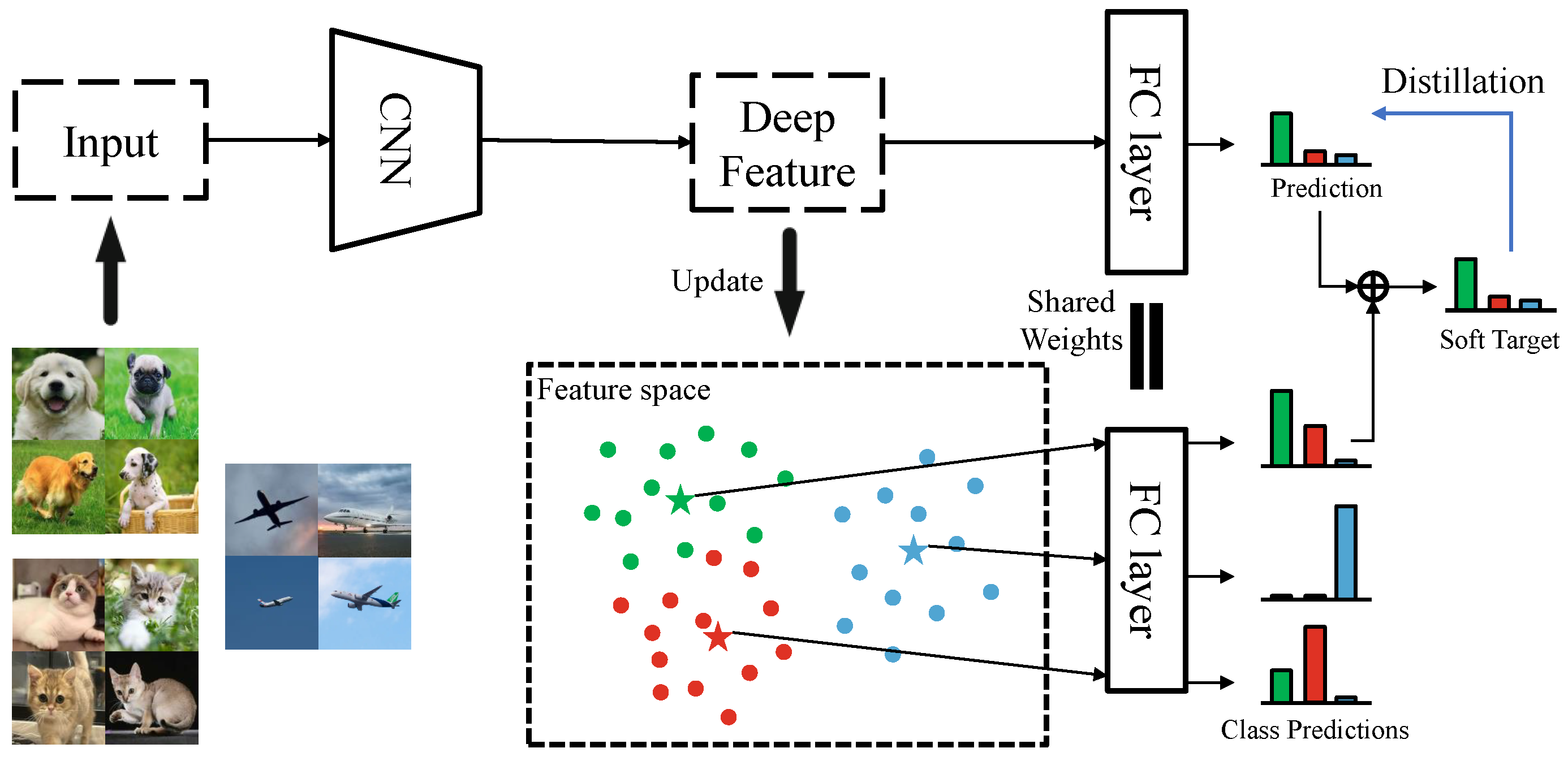
Motivated by this, we further propose a method employing ‘class centers’ [19] to dynamically acquire class predictions during training as soft targets for computing self-distillation loss, called center self-distillation (CSD), as shown in Figure 1. In this algorithm, one class corresponds to only one class prediction, which drives features under a same class move towards their ‘class centers’, thereby reducing intra-class variance. In particular, to prevent over-fitting, we generate a soft target for a given sample by moving its corresponding ‘center feature’ a certain distance towards that sample to retain some intra-class variation. The ‘class centers’ are computed in a similar way to the center loss [19], introducing almost negligible additional parameters and calculations—meaning that it can be easily applied to existing models. In contrast to earlier inter-sample self-distillation techniques, our proposed contrastive self-distillation (CSD) approach obviates the requirement for sampling an extra batch of identically labeled samples for the self-distillation process throughout training. This significant refinement leads to a marked reduction in time consumption. Furthermore, in the proposed framework, label smoothing can be interpreted as a special case of manually setting a fixed set of class centers, which provides a different explanation for why label smoothing works. To verify the generalizability of CSD, we systematically design experiments comparing it with different self-distillation models and output regularization methods. It is shown that the method has greater gains in fine-grained classes, as they are more sensitive to intra-class relations. To summarize, the main contributions of this work include the following:
- A simple visualization method is designed to observe the change in features and their gradients during training. It can provide intuition regarding how feature learning is influenced by different training methods.
- Using this visualization method, it is identified that reducing the intra-class variation in features is the key to inter-sample self-distillation.
- Base on the above finding, a simple but effective self-distillation technique, in conjunction with class centers, is proposed. It further demonstrates that reducing intra-class variance with self-distillation helps model generalization.
- The inter-sample self-distillation and our CSD are experimentally demonstrated to contribute more significantly to fine-grained classification.

Figure 1.
Illustration of center self-distillation (CSD) for three classes. The dots in the feature space indicate the deep image features, and their colors indicate the classes. The three pentagrams indicate three class centers, which are learned from the features of the training samples. The class centers will be fed into the last layer of the network to compute class predictions. These class predictions are fused with the sample predictions for generating soft targets. The final distillation is consistent with the general approach.
2. Related Work
After years of development, neural networks have been explored in many ways [20,21,22,23]. Knowledge distillation is first used for model compression [24], and its recent extensions include student matching of other statistics from teacher models rather than output predictions [25,26] such as intermediate feature representations [27,28,29] and various characteristic matrices [29,30]. When student networks themselves act as teachers, it is called self-knowledge distillation.
One approach to self-distillation directly uses the output of teachers whose structures are identical to that of the students. Born-again networks (BANs) [9] perform multi-generational self-knowledge distillation. They retain the model’s outputs from each training epoch as distillation soft targets for the next training epoch, i.e., taking the model from the previous epoch as the teacher. The teacher-free knowledge distillation (TF-KD) [31] provides two other implementations. The first one is self-training the student model for a single generation, and the second one is to manually design the target distribution as a virtual teacher model. Some other works [32,33] use models from different training periods as teachers. Gotmarec et al. [34] empirically observes that the dark knowledge transmitted by the teacher is mainly concentrated in the deeper layers and has little effect on the shallow layers. Be your own teacher (BYOT) [35] presents a self-distillation framework that boosts convolutional neural network accuracy by compressing network size, achieving accuracy improvements without increasing computational costs. This method is suitable for resource-limited devices. Zhang et al. [11] established a link between label smoothing and distillation, which is similar to our work. However, our arguments come from different theoretical perspectives and provide complementary insights. We also provide a general framework that can substantially improve the generalizability of the model.
Another approach is the mutual distillation between similar inputs. Xu et al. [36] obtained soft targets from augmented images generated by distorting the input images. They aimed to enable the network to learn common knowledge from different distorted images. Although it was somewhat effective, it had no gain on intra-class variance. Recently, class-wise self-knowledge distillation (CS-KD) [15] has focused on extracting knowledge between samples within the same class. It is implemented by additionally sampling a batch of images with the same labels as the training images in each iteration during training. This batch of images will be fed into the model, then their outputs will be used as soft targets to distill the predictions of the training samples. To further enhance the consistency of intra-class sample prediction, batch knowledge ensembling (BAKE) [16] attempts to spread the knowledge among samples within the same batch, and it achieves good performance. The authors calculated the similarity between the samples within a batch for weighing the model predictions, then the weighted predictions were summed to obtain soft targets for the samples. The core of this method is that each batch must contain a certain number of samples with the same label, which requires additional sampling. The experiments demonstrate that its most crucial role is to disseminate the knowledge of the samples with the same label. Actually, it can be considered as an enhanced version of CS-KD.
All of these methods require complex mechanisms or extra sampling as well as computation. To reduce the training costs, we analyze and explore why such methods are useful in this study and conclude that they reduce intra-class variance via mutual learning between samples. We then take this finding and propose a more concise CSD that generates soft targets based on the learned class centers, which can achieve better performance without additional sampling requirements.
3. Methods
Suppose a K-class classification task. In the network, let be the feature of the penultimate layer, where d is the feature dimension and the label of the samples is . Given a training sample, let be the feature generated by the network. Its ground-truth label is , and the corresponding one-hot coding vector is . Its logical vector is , where represents the matrix of weights and biases on the last layer of the network. Then, the prediction is , and the predicted likelihood assigns the k-th class, which can be calculated as , where corresponds to the k-th element of the logistic vector .
3.1. Visualization of Update Tendencies for Penultimate Layer Features
We design a simple visualization scheme to show how the locations of the features change in the feature space as they are trained. Assuming that the mapping from the samples to the features is robust enough, then the moving direction of the features in the feature space will be in the opposite direction of their gradient. Therefore, we can directly use the gradient to update the features to simulate the change in the features during network optimization. The steps are as follows: (1) Set up three classes and generate an equal number of random feature vectors for each class, (2) Calculate the gradients of the features based on the loss function, (3) Project the features and gradients onto the same 2D plane and visualize the updated direction of the features, and (4) Update the features using these gradients. Repeating steps 2–4 gives a clear view of how the features change during the training process.
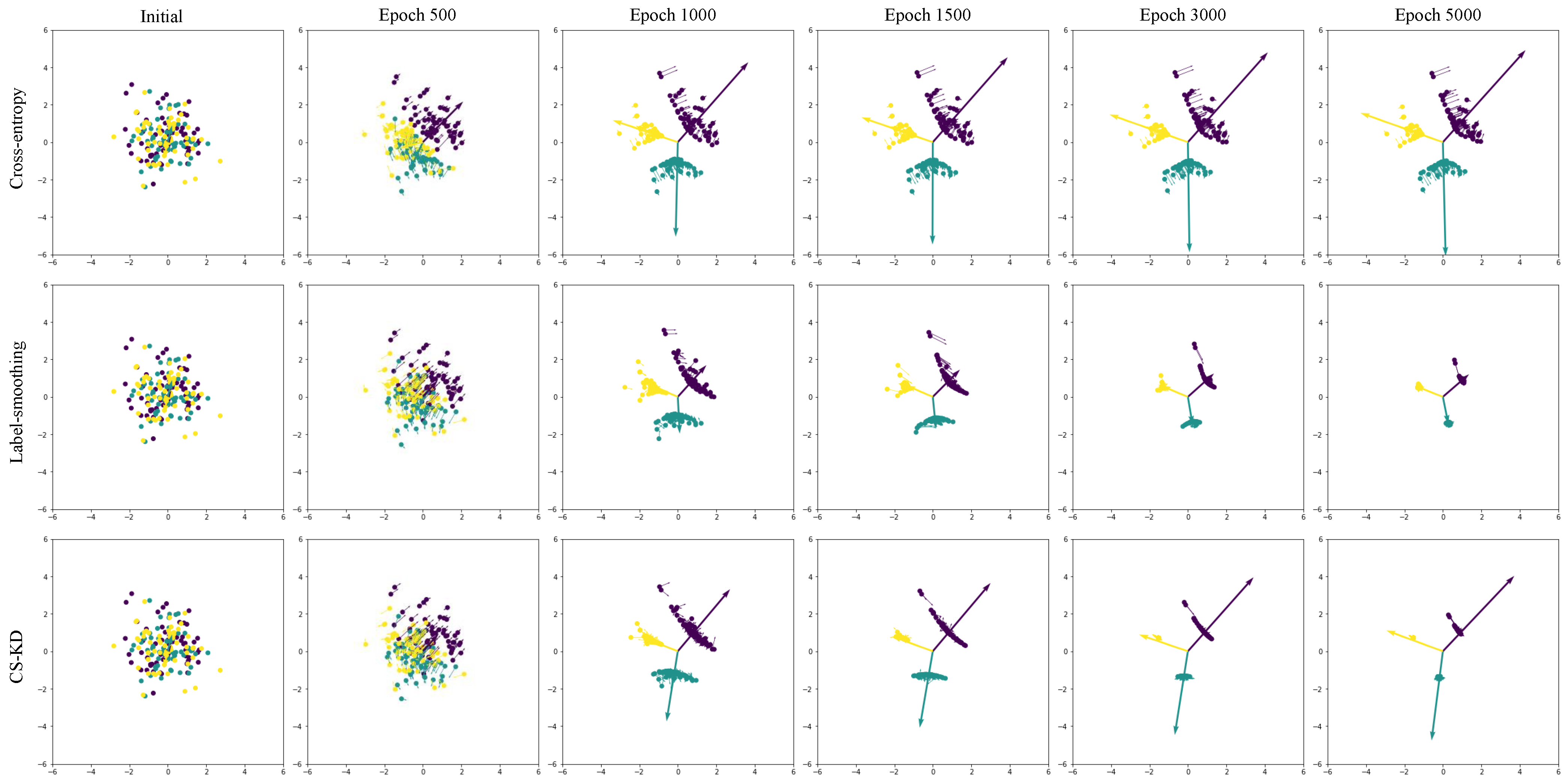
Figure 2 shows the trajectories of the features as we optimize the network using different methods. In this example, each class contains 60 features, and the dimension of the features is set to 2 for convenience (higher-dimensional features can be handled using methods such as [18,37]). It can be seen from the visualization plots that the trajectories of the feature locations are different under different loss functions. This observation highlights the distinct influences exerted by the network and aids in elucidating the function of these loss mechanisms. Subsequently, we will delve into the impacts of inter-sample self-distillation on the network, providing a detailed analysis below.
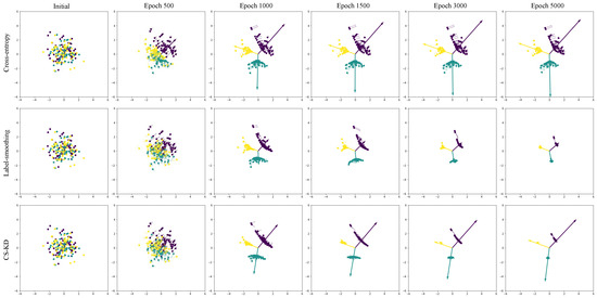
Figure 2.
Visualization of features and their updated directions. The thin arrows indicate the updated directions, whose lengths are relative (do not specify the magnitude of the updates). The thick arrows point from the origin to the coordinates of each class weight. Here, three classes in different colors totaling 180 features are randomly generated and optimized using the SGD algorithm within the framework of cross-entry (first row), label smoothing (second row), and CS-KD (third row), respectively. The positions and update directions of the features at different training epochs are shown in different columns.
3.2. How Inter-Sample Self-Distillation Affects Feature Learning
To answer this question, we revisit the general classification framework with and without inter-sample self-distillation individually.
3.2.1. Training with Cross-Entropy
Some recent studies [38,39,40] have observed that hard targets resulting from artificially annotated ground truth labels turn out to be a key factor hindering further accuracy improvements in classification models. For a common network trained using hard targets, we usually minimize the expected value of the cross-entropy between and , where is 1 for the correct class (here ) and 0 for the rest. Then, the updated direction of the feature can be obtained from its gradient. The gradient of the general cross-entropy loss acting on is , where indicates the k-th row vector of the weight matrix , corresponding to the k-th class. For a more intuitive presentation, we define the gradient component associated with the k-th class as follows:
Then, the gradient can be expressed as follows:
Here, assumes values within the interval , implying that aligns in the direction opposite to , while aligns with for instances where . This alignment is influenced by the optimization process, which inherently seeks to maximize the angular separation between the weight vectors of disparate classes. Consequently, the angle between and the aggregate vector remains consistently broad. This leads to a smaller angular divergence between and , indicating that the update trajectory of closely parallels . This dynamic introduces two primary challenges: (1) the propensity for features to be over-learned, which can compromise the model’s generalizability, and (2) updates to features within the same class tend to occur in approximately parallel directions, rendering intra-class variance heavily dependent on the initial positioning of the features.
These phenomena are visually represented in the first row of Figure 2, where certain features, initially poorly positioned, remain distant from their class counterparts throughout the training duration. Such occurrences are not uncommon, particularly in tasks characterized by significant initial intra-class variation such as fine-grained classification tasks [41,42,43], where the challenge of minimizing intra-class variance can notably impair the network’s ability to generalize. Additionally, pronounced intra-class variation results in the dispersion of similarly labeled features, adversely affecting the learning of class-specific weight vectors .
Furthermore, this examination of the impact exerted by cross-entropy loss on the spatial distribution of features also furnishes an insight into how pre-training on datasets like ImageNet [44] can enhance model generalization. This enhancement is presumably attributed to the pre-training process ameliorating the initial feature positioning, thereby facilitating a more effective learning trajectory when training on tasks with considerable intra-class variation.
3.2.2. Training with Inter-Sample Self-Distillation
Knowledge distillation introduces the concept of temperature to soften the predicted output . Its k-th element is , where denotes the hyperparameter of temperature. Let represent the soft target generated by the teacher network for . The joint minimization of the cross entropy and Kullback–Leibler divergence (KL divergence) between the predictions and the soft targets can be given as follows: , where is the weight of the two terms. Then, according to Equation (1), the gradient of feature in knowledge distillation can be computed as follows: , where and denote the k-th and i-th elements of , respectively. Generally, is a softmax output, so . Here, when we define and , we have the following:
The effects of the gradient component on the feature distribution have been discussed above. Here, we explore the role of the gradient component originating from in feature learning. For the k-th component of , if and only if . If , the angle between the feature and the weight will be updated to be larger. If , it will be updated to be smaller. This motivates and to maintain a certain positional relation in the feature space, which can penalize over-optimization. We define the logical vector satisfying as , i.e., . Then, the feature satisfying this condition must be a solution of the non-homogeneous linear equation . The equation has solutions only if is full rank (it has a unique solution if is a square matrix). The exploration into the dynamics of feature learning through supervision with hard targets reveals that such an approach causes the angles between the weights of different classes to widen, symbolized by , evolving towards a full rank matrix [45]. This progression enables the features to align more closely with their respective solutions within the feature space, thereby elucidating the contribution of knowledge distillation towards feature learning. A natural progression of this inquiry leads us to consider the scenario where samples within the same class serve as distillation targets for one another, a process herein referred to as inter-sample self-distillation.
Building upon this premise, it becomes evident that within a given class, features act as mutual solutions, converging towards one another throughout the training process. This mechanism directly addresses the limitations identified in Section 3.2.1, where it was noted that cross-entropy alone fails to adequately constrain the intra-class variance, thereby allowing samples, particularly those with suboptimal initial positions, to stray from their class centroids. Distinct from other distillation methodologies, the quintessential benefit of inter-sample self-distillation lies in its capacity to diminish the intra-class variance. This insight seamlessly bridges the concept of inter-sample self-distillation with label smoothing, which is mathematically formulated as , wherein symbolizes a uniform distribution. This distribution, , essentially acts as a constant soft label for each class, guiding the intra-class features towards a unified target, thereby mitigating intra-class discrepancies.
To elucidate the comparative effectiveness of these strategies, visual analyses were conducted, as depicted by the second and third rows in Figure 2. These visualizations highlight the reduction in intra-class variation and the subsequent consolidation of features as a result of the training process. It becomes apparent that the employment of soft targets through inter-sample self-distillation fosters more favorable inter-class relationships; a key factor in its superior performance over label smoothing across numerous practical applications. However, it is noteworthy that this advantage comes at the cost of increased training complexity, necessitated by the additional steps of sampling and predicting similar samples. Consequently, this study proposes a novel methodology aimed at amalgamating the strengths of both label smoothing and inter-sample self-distillation, with the objective of optimizing training efficiency.
3.3. Center Self-Distillation
Class centers contain comprehensive information regarding all features, and ref. [16] shows that learning knowledge from multiple samples of the same class simultaneously facilitates network generalization. Therefore, in the proposed center self-distillation (CSD), class centers are considered as an alternative to same-class samples. The purposes of designing CSD are twofold: (1) to further verify whether using the same soft target for each class can eliminate intra-class variance and improve network generalization, and (2) to eliminate the dependence of the inter-sample self-distillation method on additional sampling. As shown in Figure 1, the core of CSD is to employ class predictions generated by class centers as soft targets for knowledge distillation. Specifically, let be the class centers. Each of them will be initialized from zero. Then, the c-th class center ( belongs to the c-th class) can be updated as follows:
where controls the update rate of . The class centers are updated simultaneously with the network parameters, so we can obtain dynamic soft targets for the distillation of different samples. Here, the soft target of the c-th class is calculated according to the c-th class center as follows:
where denotes the k-th element in . Setting up soft targets in this way allows features with the same label f to have exactly the same target position in the feature space. But, complete elimination of intra-class variation can lead to over-fitting. Therefore, we offset the soft target to the corresponding feature (here, the feature is ) to preserve a certain intra-class variation:
where is the offset factor. This process encourages different features to maintain a certain individuality and prevents features from aggregating to a single point. The final overall loss of the method is as follows:
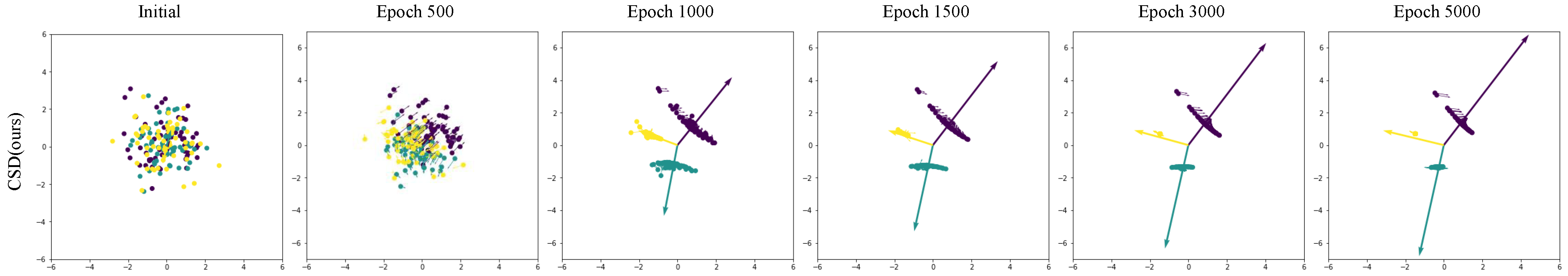
To observe the effectiveness of the method, we visualize it in Figure 3. It can be seen that it not only drives the features towards their respective class centers but also allows for some differences between features. This is the reason why it can provide better generalization on various tasks.

Figure 3.
Visualization of features and their update directions within the CSD framework.
4. Experiments
4.1. Dataset
To demonstrate our approach under the general situation of data diversity, we conducted experiments on tasks including both regular and fine-grained classification tasks. Specifically, the CIFAR100 [46] and TinyImageNet datasets were used for the regular classification tasks, and the MIT67 [47], CUB-200-2011 [41], and Stanford Dogs [48] datasets were used for the fine-grained classification tasks. Compared to traditional classification tasks, fine-grained image classification tasks have visually similar classes, and each class contains fewer training samples. The specific statistical information of all the datasets are summarized in Table 1.

Table 1.
Statistics of benchmark datasets.
4.2. Network Architectures
Two state-of-the-art convolutional neural network structures, ResNet [49] and DenseNet [50], are used here to assess our proposed method. For a fair comparison, we follow the setting of the current state-of-the-art work [15] by using standard ResNet-18 with 64 filters and DenseNet-121 with a growth rate of 32 for the 3 fine-grained datasets. For the remaining two datasets with image sizes of , PreAct ResNet-18 [51] with a modified first convolutional layer is used.
4.3. Implementation Details
In this work, the proposed framework was implemented using PyTorch [52], and all experiments were performed on a workstation equipped with an NVIDIA 3090 GPU. Following ref. [15], all the networks were trained from scratch, and the SGD algorithm was used to optimize them with a momentum of 0.9 and a weight decay of 0.0001. For all the experiments, the initial learning rate of all the models was set to 0.1. The total number of epochs was set to 200, and the learning rate was divided by 10 after 100 and 150 epochs, respectively. We set the batch size to 64 for the regular dataset and 16 for the fine-grained dataset. Standard data augmentation techniques, i.e., flipping and random cropping, were applied to all data. In the proposed method, the temperature is chosen from , and are both set to 0.9, and is chosen from . The aim of choosing the parameters is to minimize the top-1 error rate in the validation set. Each experiment was run three times. The mean and standard deviation of the results obtained from the three experiments are then reported.
4.4. Evaluation Metrics
The following four evaluation metrics are used to evaluate the various performances of the proposed method on real tasks:
(1) Top-1/5 error rate [53]. The top-k error rate is the fraction of correct labels that are not in the top-k predicted values. Its used to assess the generalization of the model. The formula is as follows:
where N is the total number of test samples, is the indicator function, which takes the value 1 if the condition inside is true, otherwise it takes the value 0; is the predicted class of the i-th sample; , , , , and are the top 5 predicted labels for the i-th sample; and is the true label for the i-th sample.
(2) Recall at k (R@k) [54]. The recall at k is the percentage of test samples with at least one of the k-nearest neighbors in the feature space that are from the same class. Here, the Euclidean distance is used to measure the distances of the penultimate layer features. The recall of the scores is used to assess the intra-class variation of the learned features.The formula for recall at k is as follows:
where |Relevant items in top k results| is the number of relevant items retrieved in the top k results. |Total number of relevant items| is the total number of relevant items in the dataset.
(3) Expected Calibration Error (ECE). ECE [55,56] measures the differences in the expectations between confidence and accuracy. The formula for ECE is as follows:
where M is the number of bins. is the set of indices of samples whose predicted probability falls into the m-th bin. n is the total number of samples. is the accuracy of the samples in the m-th bin. is the average confidence (predicted probability) of the samples in the m-th bin. Following [15], here, we set 20 bins to evaluate the impact of the proposed method on the calibration.
(4) Mean standard deviation (Mstd) [57]. Mstd is the mean mold of the standard deviations for intra-class features. We use it to evaluate the density of intra-class features. The formula for Mstd is as follows:
where N is the number of samples. is the i-th sample value. is the sample mean, defined as .
4.5. Quantitative Results
We compared our method with a variety of state-of-the-art (SOTA) methods, and the results are shown in Table 2. Specifically, these methods can be divided into the following types.
Table 2.
Top-1 error rates (%) on various image classification tasks and model architectures. The best results are in bold font.
(1) Output regularization methods. Since self-distillation can be interpreted as a regularization of the output [15], the proposed CSD is compared with some output regularization methods. Among them, AdaCos [58] and Virtual-softmax [59] maximize the angular margins by adding a cosine distance constraint and an additional virtual class, respectively. Maximum-entropy [60] regularizes the entropy to maximize the entropy of the predicted distribution. The results show that our methods, as well as the other inter-sample self-distillation methods, outperform the baselines on all five datasets, mainly because of the inter-class relationship introduced by these methods through self-distillation. Moreover, the introduced inter-class relations are dynamically optimized and gradually approach the true data distribution during training, which greatly helps to improve the generalizability of the model.
(2) Generalized self-distillation methods. A few of the most recent state-of-the-art models are compared here. Data distortion-guided self-distillation (DDGSD) [36] enforces consistent output between different data-enhanced versions. Be your own teacher (BYOT) [35] transforms the knowledge in the deeper layers of the network into shallower ones. DDGSD outperforms the output regularization method on TinyImageNet and MIT67, but it does not significantly improve the performance on the other three datasets. All the inter-sample self-distillation methods outperformed it, in contrast to inter-sample self-distillation. Although theyse methods also tap inter-class relations, what they lack is a constraint on intra-class variation.
(3) Inter-sample self-distillation methods. The existing two-sample self-distillation methods contribute significantly to image classification. CS-KD [15] randomly samples a batch of samples with the same label as the teacher in each iteration during training. BAKE [16] samples multiple batches of samples with the same label in each iteration and fuses the sample knowledge as the teacher. They outperform the above methods but also introduce complex sampling mechanisms. Our CSD explores the underlying reasons why they work and simplifies such mechanisms accordingly, outperforming them on all data sets. Comparing the three methods, CS-KD learns from another sample, BAKE learns from multiple samples at the same time, while our method goes a step further by learning from all the samples within a class at the same time, greatly exploiting the potential of samples to learn from each other.
(4) Label smoothing [18]. Label smoothing is effectively a subset of our method, where class centers are considered static. Given the variability in data distributions, label smoothing yields notable benefits for only a subset of datasets. In contrast, our contrastive self-distillation (CSD) method dynamically updates class predictions, ensuring its applicability and effectiveness across all datasets. This adaptability allows CSD to maintain an optimal performance, irrespective of the underlying data distribution, thereby providing a more universally applicable solution.
(5) Center loss [19]. Our perspective posits that inter-sample self-distillation diminishes intra-class variability, prompting a comparison between our contrastive self-distillation (CSD) approach and center loss. The superiority of our method primarily stems from the incorporation of constraints on inter-class dynamics alongside a targeted intra-class sample bias. This approach mitigates the risk of overfitting by preventing excessive clustering of intra-class features. Additionally, the emphasis on inter-class relationships fosters a more robust learning of class distributions, further enhancing model performance.
In addition, our CSD has particularly significant performance improvements on three fine-grained datasets: about 5–6% relative to SOTA with the Resnet-18 as the backbone, and about 4–8% relative to SOTA with the DenseNet-121 as the backbone. The reason for this is that our method emphasizes the control of intra-class distance and inter-class distance. Since fine-grained datasets have a higher inter-class similarity and are more sensitive to the change in intra-class distances than common datasets, they are more likely to benefit from it.
(6) Training costs. The detailed analysis and results presented in Table 3 demonstrate how the image size significantly affects the computational requirements, specifically the training time cost and memory consumption, for training a ResNet-18 model. Training the model with larger images (224 × 224 pixels) requires substantially more computational resources—132.53 s per epoch for training time and 21.84 GB of memory—compared to smaller images (32 × 32 pixels), which only need 72.87 s per epoch and 12.01 GB of memory. Furthermore, our method utilizes a single backbone for computational processes, unlike previous methods that typically rely on two independent backbones. This approach presents a significant advancement in computational efficiency, ensuring that the resource consumption for training and running the model does not escalate beyond the comparative baseline of direct training.This can be corroborated by comparing the CSB data with the backbone network data in Table 3. In essence, the method achieves a balance between maintaining a high performance in terms of accuracy and efficiency while minimizing the increase in computational demand. This balance is crucial for deep learning applications, particularly in scenarios where computational resources are limited or when optimizing for faster, more efficient model training and inference processes.
Table 3.
Training time cost and memory consumption of ResNet-18 on various image sizes.
4.6. Ablation Study
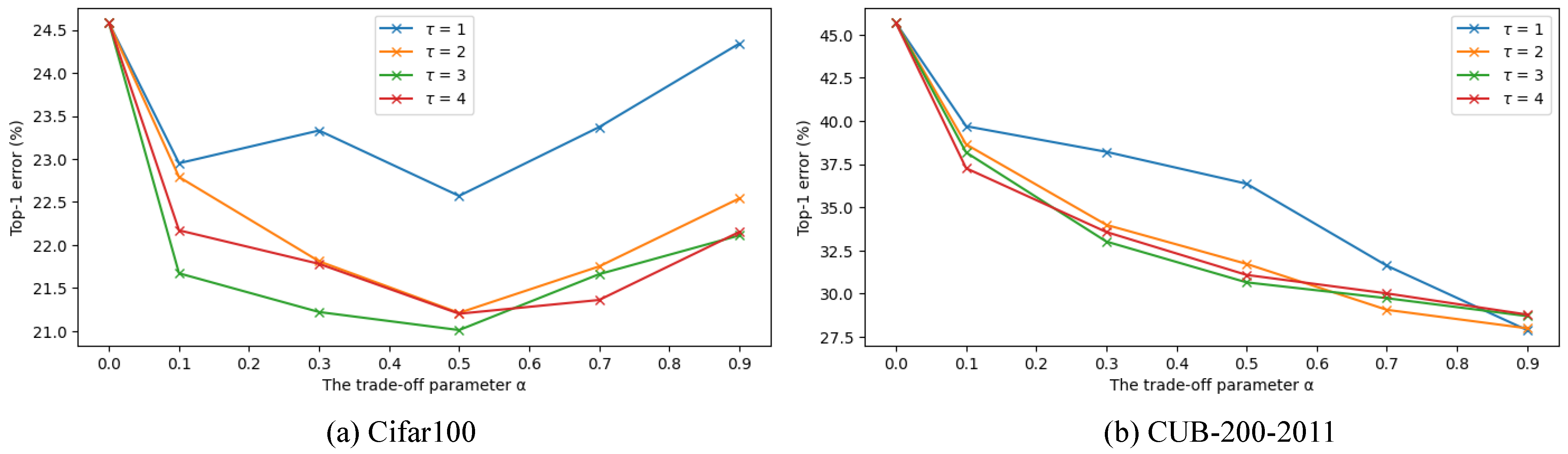
Ablation experiments are conducted for the trade-off parameter and temperature , respectively. All the experiments are implemented using ResNet-18 as the backbone. We try different values for the trade-off parameter including and the temperature including on the regular dataset CIFAR100 and the fine-grained dataset CUB-200-2011, respectively. The results are summarized in Figure 4, where equals the baseline model using cross-entropy loss.
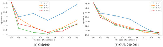
Figure 4.
Ablation analysis for the trade-off parameter and temperature . The Top-1 error rates of ResNet-18 on CIFAR100 and CUB-200-2011 are reported under the CSD settings, respectively.
It can be seen from Figure 4a that CSD achieves the best performance on CIFAR100 when distillation loss and cross-entropy loss are balanced, i.e., . The performance of the model becomes better as increases, but is insensitive at values greater than 2. The CSD exceeds the baseline across all settings, showing its good robustness. On the fine-grained task CUB-200-2011, as shown in Figure 4b, the trend of the model performance is different. The performance improves as is increased at any . The results on both datasets show that the effects of and are independent of each other. Regular tasks are suitable for larger values and a balanced distillation loss, while fine-grained tasks favor smaller values and larger distillation losses.
To further clarify the impact of different methods on the features, we measure the performance of the model based on three other aspects in Table 4:
(1) Prediction distribution. The Top-5 error rate is used here to quantitatively evaluate the prediction distribution of our model. It can be seen from Table 4 that CSD outperforms the existing methods on four datasets, especially on the CUB-200-2011, by 4% over SOTA and 12% over Cross-entropy, showing the great potential of CSD to improve the prediction distribution of the classification models. The reason is related to the inter-class relations introduced by distillation, which allow features from similar classes to hold closer positional relations in the feature space. Therefore, it can prevent the model from becoming over-optimized, enhance the generalization, and make the predictions more reasonable. This can also explain why the results of BAKE and CS-KD, which also use distillation, are also good.
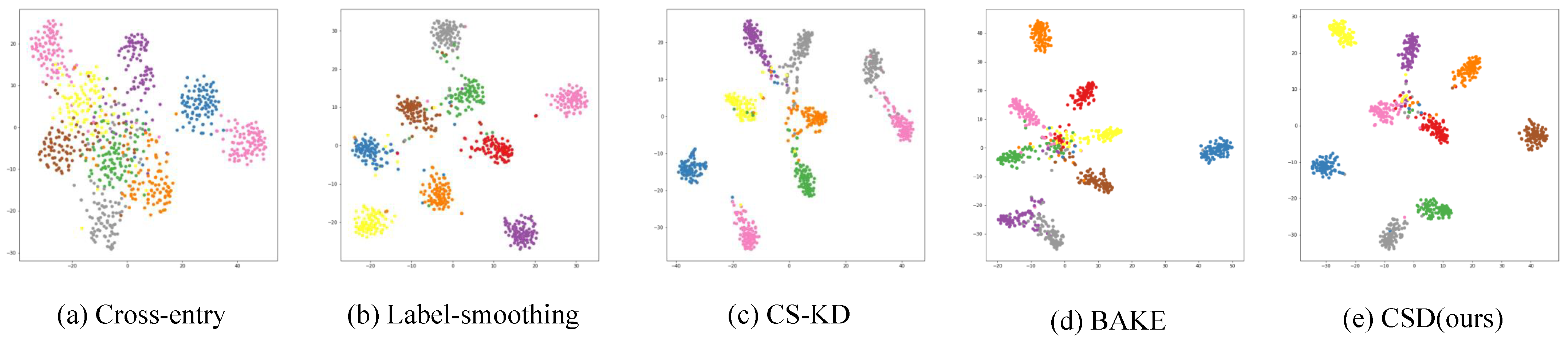
(2) Feature distribution. Here, we provide quantitative results on the metric R@1, which reflects the tightness of feature clusters [61]. A larger value of R@1 implies less inter-class crossover on the feature embedding or more distant feature clusters of different classes. As shown in Table 4, the R@1 values can be significantly improved when training ResNet-18 with CSD. The visualization of the features is shown in Figure 5. It can be seen that our method makes the features of different classes more dispersed and the features of the same class more aggregated. An important reason for this is that CSD drives same-label features to move toward their class centers, which, while not increasing the class-to-class distance, reduces the overlap between feature clusters. Fine-grained images typically have higher inter-class overlap; thus, CSD can provide greater performance improvements across several fine-grained tasks, as the results show. The experimental results shed light on the intricate dynamics of clustering observed within this study. It was noted that clusters encompassing a larger number of classes tended to demonstrate enhanced cohesiveness, effectively distinguishing themselves from neighboring clusters. This distinction is critical for the clarity and accuracy of the clustering process. Additionally, an observable dispersion within these clusters reveals that, despite the collective identity, each individual sample deviates uniquely from the cluster’s centroid. This pattern of dispersion is crucial, as it reflects the model’s adeptness at upholding the distinctiveness of each sample, thereby safeguarding its generalizability. Such a delicate equilibrium between ensuring the specificity of individual samples and their aggregation into coherent clusters underscores the sophistication of our method. It affirms the model’s robustness and adaptability in managing complex datasets, achieving a commendable harmony between the twin pillars of specificity and generalizability.
Table 4.
Top-5 error, recall at 1 (R@1) rates (%), and Mstd of ResNet-18 on various image classification tasks. The arrow on the right side of the evaluation metric indicates ascending or descending orders of the value. The best results are in bold font.
Table 4.
Top-5 error, recall at 1 (R@1) rates (%), and Mstd of ResNet-18 on various image classification tasks. The arrow on the right side of the evaluation metric indicates ascending or descending orders of the value. The best results are in bold font.
| Measurement | Method | CIFAR-100 | TinyImageNet | CUB-200-2011 | Stanford Dogs | MIT67 |
|---|---|---|---|---|---|---|
| Top-5 ↓ | Cross-entropy | 6.91±0.09 | 22.21±0.29 | 22.30±0.68 | 11.80±0.27 | 19.25±0.53 |
| AdaCos | 9.99±0.20 | 22.24±0.11 | 15.24±0.66 | 11.02±0.22 | 19.05±2.33 | |
| Virtual-softmax | 8.54±0.11 | 24.15±0.17 | 13.16±0.20 | 8.64±0.21 | 19.10±0.20 | |
| Maximum-entropy | 7.29±0.12 | 21.53±0.50 | 19.80±1.21 | 10.90±0.31 | 20.47±0.90 | |
| Label-smoothing | 7.18±0.08 | 20.74±0.31 | 22.40±0.85 | 13.41±0.40 | 19.53±0.75 | |
| CS-KD | 5.69±0.03 | 19.21±0.04 | 13.07±0.26 | 8.55±0.07 | 17.46±0.38 | |
| BAKE | 7.45±0.06 | 20.06±0.34 | 13.00±0.41 | 10.23±0.13 | 18.43±0.39 | |
| CSD (ours) | 5.34±0.09 | 19.39±0.23 | 9.49±0.24 | 7.09±0.27 | 16.77±0.71 | |
| R@1 ↑ | Cross-entropy | 61.38±0.64 | 30.59±0.42 | 33.92±1.70 | 47.51±1.02 | 31.42±1.00 |
| AdaCos | 67.95±0.42 | 44.66±0.52 | 54.86±0.24 | 58.37±0.43 | 42.39±1.91 | |
| Virtual-softmax | 68.35±0.48 | 44.69±0.58 | 55.56±0.74 | 59.71±0.56 | 44.20±0.90 | |
| Maximum-entropy | 71.51±0.29 | 39.18±0.79 | 48.66±2.10 | 60.05±0.45 | 38.06±3.32 | |
| Label-smoothing | 71.44±0.03 | 34.79±0.67 | 41.59±0.94 | 54.48±0.68 | 35.15±1.54 | |
| CS-KD | 71.15±0.15 | 47.15±0.40 | 59.06±0.38 | 62.67±0.07 | 46.74±1.48 | |
| BAKE | 71.24±0.66 | 45.23±0.34 | 62.55±0.91 | 64.72±0.43 | 46.12±0.45 | |
| CSD (ours) | 72.22±0.21 | 48.05±0.17 | 65.85±0.32 | 63.97±0.62 | 50.65±1.10 | |
| Mstd | Cross-entropy | 17.24±1.23 | 11.84±0.86 | 9.26±0.66 | 8.96±0.35 | 6.52±0.72 |
| Label-smoothing | 5.54±0.45 | 8.49±0.41 | 5.68±0.38 | 4.93±0.26 | 3.95±0.65 | |
| CS-KD | 5.91±0.34 | 5.92±0.64 | 4.18±0.29 | 3.64±0.66 | 2.91±0.31 | |
| BAKE | 3.85±0.32 | 5.42±0.48 | 3.83±0.29 | 2.70±0.19 | 2.19±0.11 | |
| CSD (ours) | 5.84±0.16 | 7.17±0.47 | 4.87±0.09 | 4.47±0.29 | 3.36±0.33 |

Figure 5.
Visualization of features on the penultimate layer. There are 9 classes of samples represented in different colors which are randomly selected from the test set of CIFAR100. Figures (a–e) show the results of various methods using ResNet-18 as the backbone.
(3) Intra-class feature variance. We used Mstd to quantify the average intra-class variance across all the classes, with smaller values indicating that features within the same class are closer to each other. As Table 4 shows, the Mstd of label-smoothing, CS-KD, BAKE, and CSD is much smaller than the baseline, indicating that inter-sample self-distillation can indeed reduce intra-class variation. The Mstd of CSD is similar to label-smoothing across almost all the datasets, which can further corroborate our view that label-smoothing can be regard as a special case of CSD. Another difference between CSD and the previous approaches is that, as shown in Equation (5), CSD generates soft targets by offsetting the class centers. This results in a slight increase in Mstd, but it helps the model to retain some intra-class feature variations, thus effectively preventing the overfitting caused by the density of intra-class features and improving the model’s generalization.
(4) λ variance. Based on Table 5, we can observe a clear trend: as the value of lambda increases from 0 to 0.9, the Top-1 error rate consistently decreases and Mstd grows. With = 0, the error rate is 24.71 ± 0.24%, indicating the baseline performance of the ResNet-18 model without any modification or additional regularization corresponding to lambda. The error rates are presented with standard deviations, indicating the variability of the model’s performance across different training runs or data subsets. The decreasing error rate with increasing lambda suggests that the modification or regularization technique associated with lambda positively impacts the model’s ability to generalize to new, unseen data, thus reducing the likelihood of incorrect predictions. This trend suggests that the parameter plays a crucial role in enhancing the model’s generalization capabilities, possibly by controlling overfitting or by encouraging the model to learn more robust features that are invariant across the CIFAR-100 dataset’s diverse set of images. Such findings are particularly relevant for deep learning researchers and practitioners aiming to optimize model performance on challenging classification tasks, as they highlight the importance of tuning hyperparameters like lambda to achieve lower error rates.
Table 5.
Top-1 error and Mstd of ResNet-18 on various lamda values in CIFAR-100 classification.
4.7. Calibration Effects
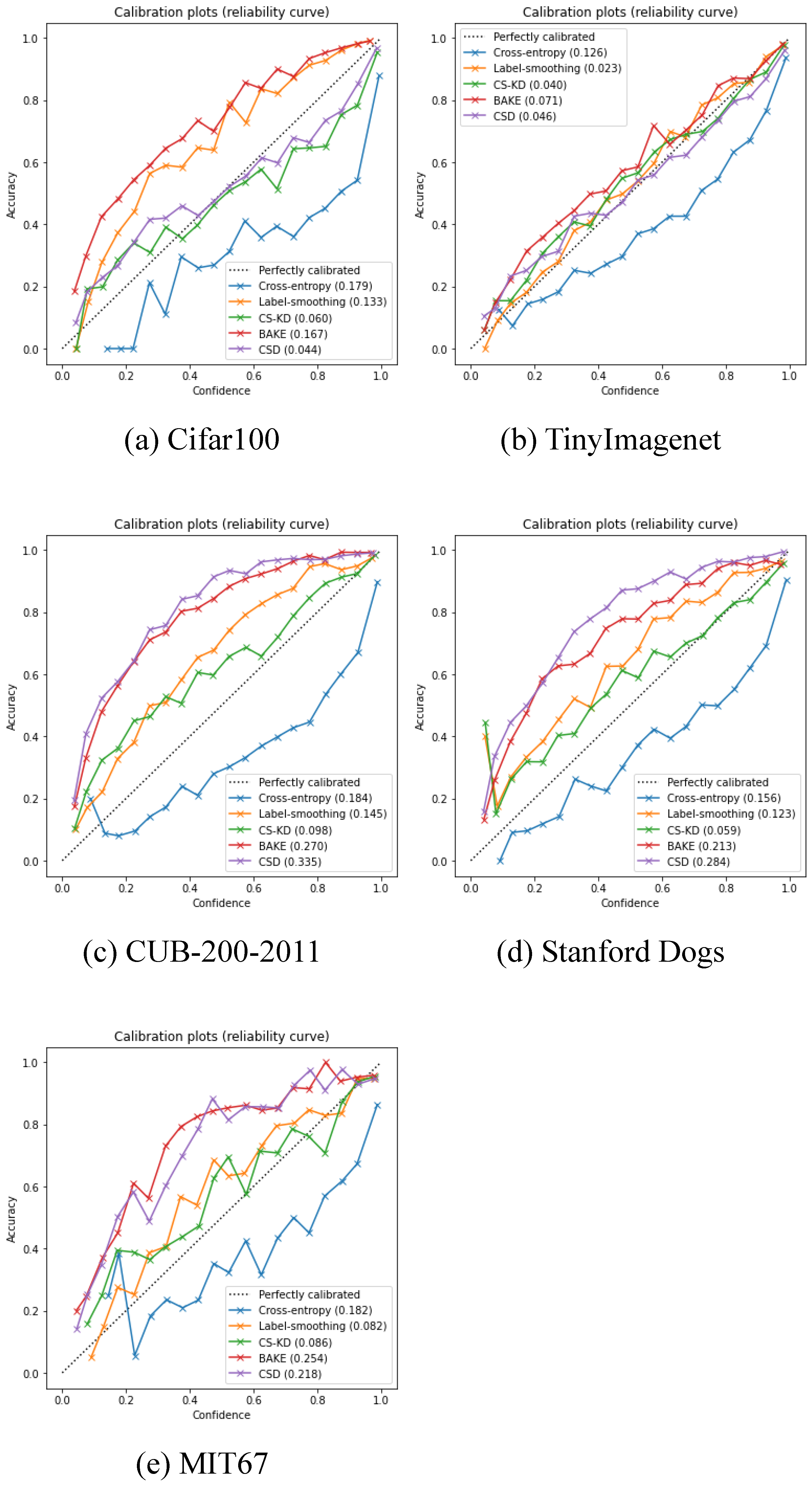
In this subsection, we assess the calibration effectiveness of the proposed CSD by ECE. For a more intuitive presentation, reliability diagrams [62] are provided in Figure 6, which plot the expected accuracy as a function of the model confidence (the dashed diagonal line indicates perfect calibration [55]). We note an interesting phenomenon: that CSD substantially improves the calibration on two regular datasets while impairing the model calibration on three fine-grained datasets. The lower calibration implies lower confidence in the predictions of the model. But it is not a bad phenomenon, because in many fine-grained tasks where the classes are very similar, we often need to know the association between the sample classes to perceive the label hierarchy [63]. The lower prediction confidence with a sufficiently high accuracy indicates that CSD can provide better class similarity relationships. In addition, as shown in Table 4, the CSD achieves the best Top-5 values on the three fine-grained datasets, indicating that the prediction confidence is spread across several similar classes, which is beneficial for the portrayal of class relations.
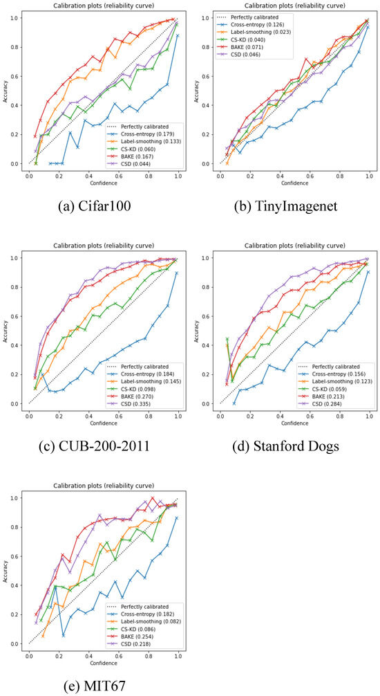
Figure 6.
Reliability diagram of multiple methods on different datasets. ECE metrics are reported in the illustrated labels.
5. Conclusions
In this study, the reason why inter-sample self-distillation can significantly improve model performance is explored. A concise method designed for visualizing feature changes shows that the key for inter-sample self-distillation is reducing intra-class variance. This method can guide the design of self-distillation methods, and this observation inspires the proposal of our CSD. Compared to previous methods, CSD does not require additional sampling and computation, which dramatically reduces the training costs of the model. Its superior performance over SOTA methods across multiple datasets demonstrates that constraining inter-sample relations can help improve model generalization. Additionally, since fine-grained tasks are more sensitive to sample relationships, experiments show that inter-sample self-distillation is more beneficial for fine-grained classification, with less gain for general image classification. We hope this exploration of intra-class variation in features can stimulate further ideas about sample relations and also prompt consideration of how sample initialization might impact network learning performance. Additionally, integrating the learning of sample relationships could potentially enhance model performance further. In addition, the computational efficiency of the CSD method and other similar methods will also be studied in follow-up research.
Author Contributions
Conceptualization, K.Z.; methodology, K.Z.; software, K.Z. and X.S.; validation, L.W.; formal analysis, K.Z.; investigation, L.Z. and X.S.; data curation, K.Z.; writing—original draft, K.Z.; writing—review and editing, L.Z. and Z.W.; visualization, K.Z.; supervision, L.Z.; project administration, L.Z.; funding acquisition, L.Z. All authors have read and agreed to the published version of the manuscript.
Funding
This work was supported by the National Natural Science Foundation for Distinguished Young Scholar of China under Grant No. 62025601.
Institutional Review Board Statement
Not applicable.
Informed Consent Statement
Not applicable.
Data Availability Statement
The original data presented in this study are openly available from CIFAR-100 at https://www.cs.toronto.edu/~kriz/cifar.html (accessed on 1 January 2024), TinyImageNet at http://cs231n.stanford.edu/tiny-imagenet-200.zip (accessed on 1 January 2024), CUB-200-2011 at https://www.vision.caltech.edu/datasets/cub_200_2011/ (accessed on 1 January 2024), Stanford Dogs at http://vision.stanford.edu/aditya86/ImageNetDogs/ (accessed on 1 January 2024), MIT67 at https://web.mit.edu/torralba/www/indoor.html (accessed on 1 January 2024).
Conflicts of Interest
The authors declare no conflicts of interest.
References
- Buciluf, C.; Caruana, R.; Niculescu-Mizil, A. Model compression. In Proceedings of the 12th ACM SIGKDD International Conference on Knowledge Discovery and Data Mining, Philadelphia, PA, USA, 20–23 August 2006; pp. 535–541. [Google Scholar]
- Hinton, G.; Vinyals, O.; Dean, J. Distilling the knowledge in a neural network. arXiv 2015, arXiv:1503.02531. [Google Scholar]
- Papernot, N.; McDaniel, P.; Wu, X.; Jha, S.; Swami, A. Distillation as a defense to adversarial perturbations against deep neural networks. In Proceedings of the 2016 IEEE Symposium on Security and Privacy (SP), San Jose, CA, USA, 22–26 May 2016; pp. 582–597. [Google Scholar]
- Yim, J.; Joo, D.; Bae, J.; Kim, J. A gift from knowledge distillation: Fast optimization, network minimization and transfer learning. In Proceedings of the IEEE Conference on Computer Vision and Pattern Recognition, Honolulu, HI, USA, 21–26 July 2017; pp. 4133–4141. [Google Scholar]
- Yu, R.; Li, A.; Morariu, V.I.; Davis, L.S. Visual relationship detection with internal and external linguistic knowledge distillation. In Proceedings of the IEEE International Conference on Computer Vision, Venice, Italy, 22–29 October 2017; pp. 1974–1982. [Google Scholar]
- Hu, B.; Zhou, S.; Xiong, Z.; Wu, F. Cross-Resolution Distillation for Efficient 3D Medical Image Registration. IEEE Trans. Circuits Syst. Video Technol. 2022, 32, 7269–7283. [Google Scholar] [CrossRef]
- Liu, T.; Lam, K.M.; Zhao, R.; Qiu, G. Deep Cross-Modal Representation Learning and Distillation for Illumination-Invariant Pedestrian Detection. IEEE Trans. Circuits Syst. Video Technol. 2022, 32, 315–329. [Google Scholar] [CrossRef]
- Ahn, S.; Hu, S.X.; Damianou, A.; Lawrence, N.D.; Dai, Z. Variational information distillation for knowledge transfer. In Proceedings of the IEEE/CVF Conference on Computer Vision and Pattern Recognition, Long Beach, CA, USA, 15–20 June 2019; pp. 9163–9171. [Google Scholar]
- Furlanello, T.; Lipton, Z.; Tschannen, M.; Itti, L.; Anandkumar, A. Born again neural networks. In Proceedings of the International Conference on Machine Learning, PMLR, Stockholm, Sweden, 10–15 July 2018; pp. 1607–1616. [Google Scholar]
- Yang, C.; Xie, L.; Qiao, S.; Yuille, A.L. Training deep neural networks in generations: A more tolerant teacher educates better students. In Proceedings of the AAAI Conference on Artificial Intelligence, Honolulu, HI, USA, 27 January–1 February 2019; Volume 33, pp. 5628–5635. [Google Scholar]
- Zhang, Z.; Sabuncu, M. Self-distillation as instance-specific label smoothing. Adv. Neural Inf. Process. Syst. 2020, 33, 2184–2195. [Google Scholar]
- Mobahi, H.; Farajtabar, M.; Bartlett, P. Self-distillation amplifies regularization in hilbert space. Adv. Neural Inf. Process. Syst. 2020, 33, 3351–3361. [Google Scholar]
- Abnar, S.; Dehghani, M.; Zuidema, W. Transferring inductive biases through knowledge distillation. arXiv 2020, arXiv:2006.00555. [Google Scholar]
- Zhou, C.; Neubig, G.; Gu, J. Understanding knowledge distillation in non-autoregressive machine translation. arXiv 2019, arXiv:1911.02727. [Google Scholar]
- Yun, S.; Park, J.; Lee, K.; Shin, J. Regularizing class-wise predictions via self-knowledge distillation. In Proceedings of the IEEE/CVF Conference on Computer Vision and Pattern Recognition, Seattle, WA, USA, 13–19 June 2020; pp. 13876–13885. [Google Scholar]
- Ge, Y.; Choi, C.L.; Zhang, X.; Zhao, P.; Zhu, F.; Zhao, R.; Li, H. Self-distillation with Batch Knowledge Ensembling Improves ImageNet Classification. arXiv 2021, arXiv:2104.13298. [Google Scholar]
- Park, W.; Kim, D.; Lu, Y.; Cho, M. Relational knowledge distillation. In Proceedings of the IEEE/CVF Conference on Computer Vision and Pattern Recognition, Long Beach, CA, USA, 15–20 June 2019; pp. 3967–3976. [Google Scholar]
- Müller, R.; Kornblith, S.; Hinton, G.E. When does label smoothing help? Adv. Neural Inf. Process. Syst. 2019, 32, 4694–4703. [Google Scholar]
- Wen, Y.; Zhang, K.; Li, Z.; Qiao, Y. A discriminative feature learning approach for deep face recognition. In Proceedings of the European Conference on Computer Vision, Amsterdam, The Netherlands, 11–14 October 2016; pp. 499–515. [Google Scholar]
- Wang, L.; Zhang, L.; Qi, X.; Yi, Z. Deep Attention-Based Imbalanced Image Classification. IEEE Trans. Neural Netw. Learn. Syst. 2021, 33, 3320–3330. [Google Scholar] [CrossRef] [PubMed]
- Zhang, L.; Yi, Z.; Amari, S.I. Theoretical study of oscillator neurons in recurrent neural networks. IEEE Trans. Neural Netw. Learn. Syst. 2018, 29, 5242–5248. [Google Scholar] [CrossRef] [PubMed]
- Qi, X.; Zhang, L.; Chen, Y.; Pi, Y.; Chen, Y.; Lv, Q.; Yi, Z. Automated diagnosis of breast ultrasonography images using deep neural networks. Med. Image Anal. 2019, 52, 185–198. [Google Scholar] [CrossRef] [PubMed]
- Wang, Z.; Shu, X.; Chen, C.; Teng, Y.; Zhang, L.; Xu, J. A semi-symmetric domain adaptation network based on multi-level adversarial features for meningioma segmentation. Knowl.-Based Syst. 2021, 228, 107245. [Google Scholar] [CrossRef]
- Ba, J.; Caruana, R. Do deep nets really need to be deep? Adv. Neural Inf. Process. Syst. 2014, 27, 2654–2662. [Google Scholar]
- Zhang, K.; Zhang, C.; Li, S.; Zeng, D.; Ge, S. Student Network Learning via Evolutionary Knowledge Distillation. IEEE Trans. Circuits Syst. Video Technol. 2022, 32, 2251–2263. [Google Scholar] [CrossRef]
- Cui, X.; Wang, C.; Ren, D.; Chen, Y.; Zhu, P. Semi-supervised Image Deraining Using Knowledge Distillation. IEEE Trans. Circuits Syst. Video Technol. 2022, 32, 8327–8341. [Google Scholar] [CrossRef]
- Adriana, R.; Nicolas, B.; Ebrahimi, K.S.; Antoine, C.; Carlo, G.; Yoshua, B. Fitnets: Hints for thin deep nets. Proc. ICLR 2015, 2. [Google Scholar] [CrossRef]
- Heo, B.; Kim, J.; Yun, S.; Park, H.; Kwak, N.; Choi, J.Y. A comprehensive overhaul of feature distillation. In Proceedings of the IEEE/CVF International Conference on Computer Vision, Seoul, Republic of Korea, 27 October–2 November 2019; pp. 1921–1930. [Google Scholar]
- Srinivas, S.; Fleuret, F. Knowledge transfer with jacobian matching. In Proceedings of the International Conference on Machine Learning, PMLR, Stockholm, Sweden, 10–15 July 2018; pp. 4723–4731. [Google Scholar]
- Wang, Z.; Shu, X.; Wang, Y.; Feng, Y.; Zhang, L.; Yi, Z. A feature space-restricted attention attack on medical deep learning systems. IEEE Trans. Cybern. 2022, 53, 5323–5335. [Google Scholar] [CrossRef] [PubMed]
- Yuan, L.; Tay, F.E.; Li, G.; Wang, T.; Feng, J. Revisiting knowledge distillation via label smoothing regularization. In Proceedings of the IEEE/CVF Conference on Computer Vision and Pattern Recognition, Seattle, WA, USA, 13–19 June 2020; pp. 3903–3911. [Google Scholar]
- Yang, C.; Xie, L.; Su, C.; Yuille, A.L. Snapshot distillation: Teacher-student optimization in one generation. In Proceedings of the IEEE/CVF Conference on Computer Vision and Pattern Recognition, Long Beach, CA, USA, 15–20 June 2019; pp. 2859–2868. [Google Scholar]
- Kim, K.; Ji, B.; Yoon, D.; Hwang, S. Self-knowledge distillation with progressive refinement of targets. In Proceedings of the IEEE/CVF International Conference on Computer Vision, Montreal, BC, Canada, 11–17 October 2021; pp. 6567–6576. [Google Scholar]
- Gotmare, A.; Keskar, N.S.; Xiong, C.; Socher, R. A Closer Look at Deep Learning Heuristics: Learning rate restarts, Warmup and Distillation. In Proceedings of the International Conference on Learning Representations, New Orleans, LA, USA, 6–9 May 2019. [Google Scholar]
- Zhang, L.; Song, J.; Gao, A.; Chen, J.; Bao, C.; Ma, K. Be your own teacher: Improve the performance of convolutional neural networks via self distillation. In Proceedings of the IEEE/CVF International Conference on Computer Vision, Seoul, Republic of Korea, 27 October–2 November 2019; pp. 3713–3722. [Google Scholar]
- Xu, T.B.; Liu, C.L. Data-distortion guided self-distillation for deep neural networks. In Proceedings of the AAAI Conference on Artificial Intelligence, Honolulu, HI, USA, 27–1 February 2019; Volume 33, pp. 5565–5572. [Google Scholar]
- Van der Maaten, L.; Hinton, G. Visualizing data using t-SNE. J. Mach. Learn. Res. 2008, 9, 2579–2605. [Google Scholar]
- Bagherinezhad, H.; Horton, M.; Rastegari, M.; Farhadi, A. Label refinery: Improving imagenet classification through label progression. arXiv 2018, arXiv:1805.02641. [Google Scholar]
- Beyer, L.; Hénaff, O.J.; Kolesnikov, A.; Zhai, X.; Oord, A.v.D. Are we done with imagenet? arXiv 2020, arXiv:2006.07159. [Google Scholar]
- Yun, S.; Oh, S.J.; Heo, B.; Han, D.; Choe, J.; Chun, S. Re-labeling imagenet: From single to multi-labels, from global to localized labels. In Proceedings of the IEEE/CVF Conference on Computer Vision and Pattern Recognition, Nashville, TN, USA, 20–25 June 2021; pp. 2340–2350. [Google Scholar]
- Wah, C.; Branson, S.; Welinder, P.; Perona, P.; Belongie, S. The Caltech-Ucsd Birds-200-2011 Dataset; CNS-TR-2011-001; California Institute of Technology: Pasadena, CA, USA, 2011. [Google Scholar]
- Maji, S.; Rahtu, E.; Kannala, J.; Blaschko, M.; Vedaldi, A. Fine-grained visual classification of aircraft. arXiv 2013, arXiv:1306.5151. [Google Scholar]
- Krause, J.; Stark, M.; Deng, J.; Li, F.-F. 3D object representations for fine-grained categorization. In Proceedings of the IEEE International Conference on Computer VISION Workshops, Sydney, Australia, 1–8 December 2013; pp. 554–561. [Google Scholar]
- Deng, J.; Dong, W.; Socher, R.; Li, L.J.; Li, K.; Li, F.-F. Imagenet: A large-scale hierarchical image database. In Proceedings of the 2009 IEEE Conference on Computer Vision and Pattern Recognition, Miami, FL, USA, 20–25 June 2009; pp. 248–255. [Google Scholar]
- Martin, C.H.; Mahoney, M.W. Implicit self-regularization in deep neural networks: Evidence from random matrix theory and implications for learning. J. Mach. Learn. Res. 2021, 22, 1–73. [Google Scholar]
- Krizhevsky, A.; Hinton, G. Learning multiple layers of features from tiny images. In Handbook of Systemic Autoimmune Diseases; Elsevier: Amsterdam, The Netherlands, 2009; Volume 1, p. 4. [Google Scholar]
- Quattoni, A.; Torralba, A. Recognizing indoor scenes. In Proceedings of the 2009 IEEE Conference on Computer Vision and Pattern Recognition, Miami, FL, USA, 20–25 June 2009; pp. 413–420. [Google Scholar]
- Khosla, A.; Jayadevaprakash, N.; Yao, B.; Li, F.F. Novel dataset for fine-grained image categorization: Stanford dogs. In Proceedings of the CVPR Workshop on Fine-Grained Visual Categorization (FGVC), Citeseer, 2011; Volume 2. [Google Scholar]
- He, K.; Zhang, X.; Ren, S.; Sun, J. Deep residual learning for image recognition. In Proceedings of the IEEE Conference on Computer Vision and Pattern Recognition, Las Vegas, NV, USA, 27–30 June 2016; pp. 770–778. [Google Scholar]
- Huang, G.; Liu, Z.; Van Der Maaten, L.; Weinberger, K.Q. Densely connected convolutional networks. In Proceedings of the IEEE Conference on Computer Vision and Pattern Recognition, Honolulu, HI, USA, 21–26 July 2017; pp. 4700–4708. [Google Scholar]
- He, K.; Zhang, X.; Ren, S.; Sun, J. Identity mappings in deep residual networks. In Proceedings of the European Conference on Computer Vision, Amsterdam, The Netherlands, 11–14 October 2016; pp. 630–645. [Google Scholar]
- Paszke, A.; Gross, S.; Massa, F.; Lerer, A.; Bradbury, J.; Chanan, G.; Killeen, T.; Lin, Z.; Gimelshein, N.; Antiga, L.; et al. Pytorch: An imperative style, high-performance deep learning library. Adv. Neural Inf. Process. Syst. 2019, 32, 8026–8037. [Google Scholar]
- Krizhevsky, A.; Sutskever, I.; Hinton, G.E. Imagenet classification with deep convolutional neural networks. Adv. Neural Inf. Process. Syst. 2012, 25. Available online: https://proceedings.neurips.cc/paper_files/paper/2012/file/c399862d3b9d6b76c8436e924a68c45b-Paper.pdf (accessed on 19 July 2024). [CrossRef]
- Kumar, A.; Singh, S.S.; Singh, K.; Biswas, B. Link prediction techniques, applications, and performance: A survey. Phys. A Stat. Mech. Its Appl. 2020, 553, 124289. [Google Scholar] [CrossRef]
- Guo, C.; Pleiss, G.; Sun, Y.; Weinberger, K.Q. On calibration of modern neural networks. In Proceedings of the International Conference on Machine Learning, PMLR, Sydney, Australia, 6–11 August 2017; pp. 1321–1330. [Google Scholar]
- Naeini, M.P.; Cooper, G.; Hauskrecht, M. Obtaining well calibrated probabilities using bayesian binning. In Proceedings of the Twenty-Ninth AAAI Conference on Artificial Intelligence, Austin, TX, USA, 25–30 January 2015. [Google Scholar]
- Lee, D.K.; In, J.; Lee, S. Standard deviation and standard error of the mean. Korean J. Anesthesiol. 2015, 68, 220–223. [Google Scholar] [CrossRef] [PubMed]
- Zhang, X.; Zhao, R.; Qiao, Y.; Wang, X.; Li, H. Adacos: Adaptively scaling cosine logits for effectively learning deep face representations. In Proceedings of the IEEE/CVF Conference on Computer Vision and Pattern Recognition, Long Beach, CA, USA, 15–20 June 2019; pp. 10823–10832. [Google Scholar]
- Chen, B.; Deng, W.; Shen, H. Virtual class enhanced discriminative embedding learning. Adv. Neural Inf. Process. Syst. 2018, 31. Available online: https://proceedings.neurips.cc/paper_files/paper/2018/file/d79aac075930c83c2f1e369a511148fe-Paper.pdf (accessed on 19 July 2024).
- Dubey, A.; Gupta, O.; Raskar, R.; Naik, N. Maximum-entropy fine grained classification. Adv. Neural Inf. Process. Syst. 2018, 31. Available online: https://proceedings.neurips.cc/paper_files/paper/2018/file/0c74b7f78409a4022a2c4c5a5ca3ee19-Paper.pdf (accessed on 19 July 2024).
- Zhou, W.; Li, H.; Tian, Q. Recent advance in content-based image retrieval: A literature survey. arXiv 2017, arXiv:1706.06064. [Google Scholar]
- Niculescu-Mizil, A.; Caruana, R. Predicting good probabilities with supervised learning. In Proceedings of the 22nd international Conference on Machine Learning, Bonn, Germany, 7–11 August 2005; pp. 625–632. [Google Scholar]
- Chang, D.; Pang, K.; Zheng, Y.; Ma, Z.; Song, Y.Z.; Guo, J. Your “Flamingo” is My “Bird”: Fine-Grained, or Not. In Proceedings of the IEEE/CVF Conference on Computer Vision and Pattern Recognition, Nashville, TN, USA, 20–25 June 2021; pp. 11476–11485. [Google Scholar]
Disclaimer/Publisher’s Note: The statements, opinions and data contained in all publications are solely those of the individual author(s) and contributor(s) and not of MDPI and/or the editor(s). MDPI and/or the editor(s) disclaim responsibility for any injury to people or property resulting from any ideas, methods, instructions or products referred to in the content. |
© 2024 by the authors. Licensee MDPI, Basel, Switzerland. This article is an open access article distributed under the terms and conditions of the Creative Commons Attribution (CC BY) license (https://creativecommons.org/licenses/by/4.0/).