Abstract
In the present study, flood hazard susceptibility maps generated using various distance measures in the Technique for Order Preference by Similarity to an Ideal Solution (TOPSIS) were analyzed. Widely applied distance measures such as Euclidean, Manhattan, Chebyshev, Jaccard, and Soergel were used in TOPSIS to generate flood hazard susceptibility maps of the Gökırmak sub-basin located in the Western Black Sea Region, Türkiye. A frequency ratio (FR) and weight of evidence (WoE) were adapted to hybridize the nine flood conditioning factors considered in this study. The Receiver Operating Characteristic (ROC) analysis and Seed Cell Area Index (SCAI) were used for the validation and testing of the generated flood susceptibility maps by extracting 70% and 30% of the inventory data of the generated flood susceptibility map for validation and testing, respectively. When the Area Under Curve (AUC) and SCAI values were examined, it was found that the Manhattan distance metric hybridized with the FR method gave the best prediction results with AUC values of 0.904 and 0.942 for training and testing, respectively. Furthermore, the natural break method was found to give the best predictions of the flood hazard susceptibility classes. So, the Manhattan distance measure could be preferred to Euclidean for flood susceptibility mapping studies.
1. Introduction
Floods are among the most dangerous natural disasters caused by various reasons such as short periods of excessive rainfall, hurricanes, sudden snowmelt, dam failures, etc. Hydro-meteorological factors (air temperature, relative humidity, evapotranspiration, etc.) [1], anthropogenic issues (unplanned urbanization, overexploitation of natural resources, land-use change, etc.) [2,3], and geomorphic parameters of the watersheds (drainage density, stream frequency, shape factor, etc.) [4] affect the frequency and magnitude of the floods. The increase in intensity and frequency of precipitation caused many flood disasters in different locations over the globe and is excepted to continue due to climate change [5]. As a result, severity, interval, and occurrence of the flash floods are also expected to increase. Hence, flooding presents a serious threat to the environment, human beings, and infrastructures. Accordingly, research concentrated on development of various flood assessments such as hazard, risk, vulnerability, and susceptibility maps of floods in order to forecast the extent of flooding, to distinguish the flood-prone areas, to estimate the value of assets subjected to a flood hazard and possible economic loss, and to develop management plans and strategies.
A massive amount of datasets is commonly necessary to prepare such flood-related assessments of a region. Traditional observational methods can be expensive, challenging, and inadequate to provide such datasets [6]. So, two very useful and cost-effective tools, remote sensing (RS) and a geographic information system (GIS), became vital instruments for flood-related studies, enabling time and cost-effective collection and processing massive and detailed geospatial data even in inaccessible regions. RS has been widely used in determining the flood extent [7], monitoring the flood events [8,9,10], mapping of the in-undated regions [11,12], and identifying damages in flood-induced areas [13,14].
Recent studies on generating flood-related assessments, as aforementioned, are mainly concentrated on using machine learning, bivariate statistics, and multi-criteria decision-making (MCDM) algorithms. Artificial neural networks (ANNs) [15,16,17,18], decision trees (DTs) [19,20,21], and support vector machine (SVM) [22,23,24] are among the favored machine learning algorithms. Considering the statistical methods in flood susceptibility assessments, the most widely used technique is the bivariate statistical analysis [25,26,27], which involves the frequency ratio (FR) method [28,29,30], weights of evidence (WoEs) [31,32], statistical index (SI) [33,34], certainty factor (CF) [35,36,37], belief function (Bel) [38], and index of entropy (IoE) [39]. However, the complex non-linear nature of flooding contradicts the statistical methods because of their dependence on variables obtained from linear assumptions [40,41,42]. In flood-related studies, multi-criteria decision-making (MCDM) models have become widely preferred due to their high efficiency in making decisions based on multiple criteria [43,44]. They are used to delineate flood hazard zonation [45], flood susceptibility mapping [46], flood vulnerability mapping [47], flood risk mapping [48], flash flood analysis [42], and flood forecasting [49]. Regarding the MCDM, the most commonly used techniques are Analytical Hierarchy Process (AHP) [50,51,52], VIseKriteri-jumska Optimizacija I Kompromisno Resenje (VIKOR) [53], and Technique for Order of Prioritization by Similarity to Ideal Solution (TOPSIS) [54,55,56,57,58,59,60].
According to the TOPSIS method, the alternatives that yield the shortest distance from the positive ideal solution (PIS) and furthest from the negative ideal solution (NIS) are targeted. Then, the relative risk assessment is achieved by calculating the relative proximity between alternatives and the ideal solutions. However, one major limitation of this method is the lack of a weight calculation module. So, in recent years, other MCDM approaches, such as AHP, have been integrated to retrieve weight values, yielding a hybrid AHP-TOPSIS approach. Thus, TOPSIS has gained a wider usage in flood risk assessment by assessing the relative risks based on attribute value information and thus facilitating the identification of more potential flood risks [53,54,61,62,63,64]. According to this method, a distance measure is required to compute the distance from the PIS and NIS for each alternative. Thus, distance metrics offer a basis for assessing the difference or similarity between data points, enabling meaningful comprehension to be obtained from data. Therefore, they affect the accuracy of the results. In the literature, there are various distance measures that can be grouped under various hypotheses and behaviors. For instance, Euclidean, Manhattan, and Chebyshev are grouped in Minkowski’s metrics, while Jaccard and cosine similarity is a geometry-based metric and is grouped under the inner product family. Some metrics, such as Pearson, are derived from correlation metrics, while some metrics, such as Soergel, can be coherently clustered [65,66]. The choice of a distance measure to be used is crucial since it directly affects the prediction capability of the model. The most widely used distance measure in flood-related studies is the Euclidean distance [67,68]. The literature review showed that there is a very limited number of studies on the performance evaluation of the distance measures [69,70], but none on flood susceptibility mapping to the best knowledge of the authors. Since ranking depends on this computed distance, it is crucial to integrate the most appropriate distance measure considering the problem to be solved and the MCDM approach to be used. Costache et al. [71] used the Euclidean distance in the k-Nearest Neighbor model and noted that other distance measures, such as Manhattan, Chebyshev, and Hamming, could be more suitable for other model settings with no detailed explanation. So, the main goal of this study is to evaluate the performance of different distance measures chosen according to their wide usage or their origins, such as Manhattan, Euclidean, Chebyshev, Jaccard, and Soergel distances, on the generated flood susceptibility maps by using the TOPSIS method in order to further improve the capability of the model outcomes. The frequency ratio (FR) and the weight of evidence (WoE) values are used for the hybridization of the conditioning factors for the creation of a decision-making matrix in the TOPSIS method. After the calculation of closeness coefficient values, flood susceptibility maps were generated. Furthermore, the performance of the predicted maps was evaluated by the application of the Receiver Operating Characteristic (ROC) curve analysis. Flood hazard potential classes were estimated using the four classification methods named equal, quantile, natural break, and geometric intervals to evaluate the outputs by the Seed Cell Area Index (SCAI) analysis.
2. Materials and Methods
2.1. Description of the Study Area
The Gökırmak sub-basin, situated in the Western Black Sea Basin, was chosen as the study area, as shown in Figure 1.
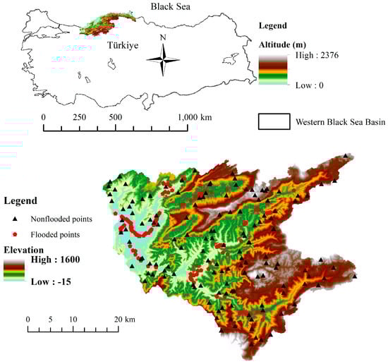
Figure 1.
Location of study area and randomly selected flooded and non−flooded points.
The study area is located between 443,833–498,543 X and 4,578,260–4,624,360 Y (UTM ED50, Zone 36 N) in the northern part of Türkiye. In the sub-basin, the Gökırmak Stream, which is the largest tributary of the Bartın Stream, collects water from an altitude of 1600 m. The Gökırmak sub-basin has an approximate drainage area of 1375 km2 and steep topography with an average gradient of 35%. In the Western Black Sea Basin, the annual average rainfall depth is 811 mm, and the annual flow volume is 9.93 km3 [72]. The region has a borderline humid subtropical and oceanic climate, with precipitation being observed in all seasons, with snowfall at high altitudes only during the winter season. In the basin, flash floods caused by snowmelt due to sudden temperature rises and extreme rainfall in a short period of time are common. Hydrologic soil groups in the basin are classified as B, C, and D. The curve number value typically ranges from 55 to 98, with an average value of 75.8. Thus, a significant amount of the rainfall in the basin continues as runoff. Furthermore, the basin is affected by rapid unplanned urbanization and industrialization.
2.2. Methodology
Figure 2 shows the methodology adopted in this study to obtain flood hazard susceptibility maps.
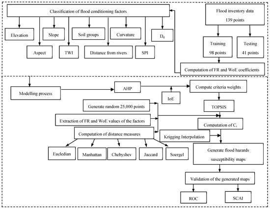
Figure 2.
Flood hazard susceptibility mapping methodology.
2.3. Data
In the current study, two main groups of data are used. The first group of data involves the spatial distribution of flood conditioning factors that are considered to directly affect the occurrence of flash floods, which are derived from the DEM, geological, and anthropogenic factors of the basin. The second group of data consists of the flood inventory data, which include hazards that occurred at past flood events. This inventory was gathered from local authorities and previous studies of the region.
2.3.1. Flood Inventory Data
The flood inventory data of an area present crucial information about past flood events, such as the date of occurrence, locations, and their impacts on the area. Today, geographic information systems are very useful tools to generate these maps [73]. However, other sources such as in situ data collection, related past reports and maps, and satellite spatial images can be used. In this study, the flood inventory map was generated based on past flood events’ data gathered from various authorities. A total of 139 points were considered from past flood events for the generation and testing of the flood susceptibility map. Out of these 139 points, 98 were randomly selected for training, while the test of the 41 points was used for the validation of the generated flood susceptibility map. Non-flooded points were mainly chosen randomly by using ArcGIS 10.8.2 and generally taking into consideration the weak possibility of the point being flooded. Figure 1 shows randomly selected flooded (n = 139) and non-flooded (n = 139) points extracted for training and testing of the flood susceptibility map of the sub-basin.
2.3.2. Flood Conditioning Factors
The accuracy of the flood susceptibility maps greatly depends on the precision of the flood inventory data and the selected flood conditioning factors. In the current study, previous reports, research, literature, and experiences of the authors were considered to determine the flood conditioning factors that have an important impact on flash floods. So, nine flood conditioning factors, namely elevation, slope, curvature, aspect, Topographic Wetness Index (TWI), Stream Power Index (SPI), soil groups, drainage density (Dd), and distance from the stream, were selected to generate the flood susceptibility map as shown in Figure 3.
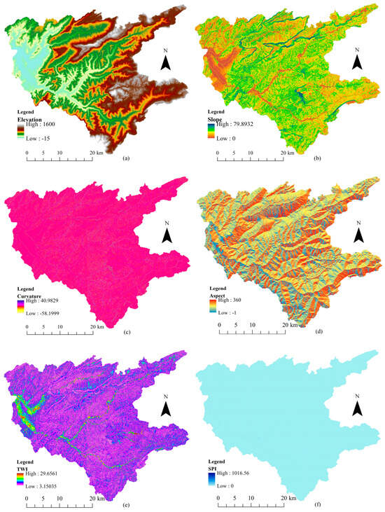
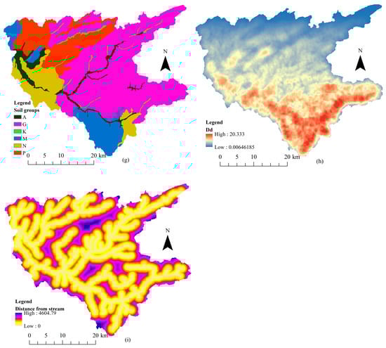
Figure 3.
Flood conditioning factors of Gökırmak watershed (a) elevation, (b) slope, (c) curvature, (d) aspect, (e) TWI, (f) SPI, (g) soil groups, (h) Dd, (i) distance from stream.
Apart from soil groups, all flood conditioning factors were processed in ArcGIS using Digital Elevation Model (DEM) with a resolution of 10 m obtained from 1: 25,000-scaled topographic maps. Studies showed that a flood susceptibility map generated by using a DEM with finer cell sizes may provide limited improvement in the predictions when compared with coarser cell sizes, but cannot significantly affect the accuracy of predictions [74,75]. Only DEM of the Gökırmak sub-basin was used to obtain slope, aspect, and curvature grids, while after filling sinks’ operation of DEM, flow direction and accumulation cells were determined. The great soil groups that are present in the basin are alluvial (A), gray-brown podzolic (G), colluvial (K), brown forest (M), non-calcareous brown forest (N), and red yellow podzolic (P), which were considered. Then, the TWI and SPI were determined as a function of flow accumulation and slope grids. The stream network of the watershed was extracted based on the threshold value of the flow accumulation cell to determine the flood conditioning factor of distance from the stream and Dd.
In the current study, conditioning factors such as elevation, slope, distance from the stream, TWI, SPI, and Dd were categorized using the natural break method in five sub-classes, whereas the supervised classification method was used to categorize the rest of the factors such as aspect, curvature, and soil groups. Aspect was classified based on the cardinal and inter-cardinal directions. Curvature is classified based on the curvature properties of the surface, which are flat (−0.05–0.05), convex (>0.5), and concave (<−0.05). Soil groups were classified based on the six great soil groups in the catchment since they do not contain any numerical values. This supervised classification enabled the significant interpretation of the flash floods based on the curvature classes, directions, and soil groups.
2.4. Flood Susceptibility Mapping
In the current study, the frequency ratio (FR) and weights of evidence (WoEs) were used to hybridize the classes of flood conditioning factors to be used in the decision matrix in TOPSIS. Index of entropy (IoE) values of the flood condition factors were used to determine the weights of the factors to be used in the AHP method. Five distance measures as Euclidean, Manhattan, Chebyshev, Jaccard, and Soergel were implemented to determine the closeness coefficient values in TOPSIS. Closeness coefficients calculated at randomly selected points were interpolated throughout the basin using the Krigging method to generate the flood susceptibility maps. Estimations were validated using the Receiver Operating Characteristic (ROC) analysis and the Seed Cell Area Index (SCAI) values for both training and testing points.
2.4.1. Frequency Ratio (FR)
It is vital to identify the conditioning factors that affect a flood when generating the flood susceptibility map of a region. So, by using past flood events and those attributed flood conditioning factors, a relationship between flood hazard pixels and the related conditioning factors can be derived. FR at a class of a flood conditioning factor is defined as the ratio of the flooded point percent at a class to the class pixel percent in the domain [62]. In the current study, FR, which is one of the most common statistical methods, was used to hybridize each class of flood conditioning factors.
2.4.2. Weights of Evidence (WoEs)
WoE, a bivariate statistical method, is based on a log-linear Bayesian theorem. Since it is a data-driven model, it has become a widely used model in the preparation of susceptibility maps of natural disasters. According to the WoE, a relationship between the flood event and the conditioning factors is defined such that positive (W+) and negative weights (W−) correspond to the occurrence and non-occurrence of flood hazards, taking into account the flood inventory data at a prescribed class of a flood conditioning factor [76], given as
where P is the conditional probability, and A is the presence of flood pixels at B flood conditioning factor, while the line bar denotes the absence of A and B. In the current study, W was used to hybridize each class of the flood conditioning factors.
Equations (1) and (2) are used to compute the variances of Wi+ and Wi− in terms of the number of flooded and non-flooded pixels in a class (N). Contrast (C) is determined by taking the difference between Wi+ and Wi−, and its standard deviation is given in Equation (5). So, the weight of each class (W) can be calculated by Equation (6).
2.4.3. Analytical Hierarchy Process (AHP)
AHP is one of the most frequently used methods of multi-criteria decision-making, enabling the assignment of different weight values to the thematic layers of each conditioning factor to display their relative influences [77]. In this study, the criteria weights of each conditioning factor were implemented by considering Wj values obtained from the index of entropy (IoE) and compound factor. Wj values were sorted in ascending order by grading from 1 to 9. These compound values were used to generate a pair-wise comparison matrix of flood conditioning factors according to Saaty’s [78] scale, from which the criteria weight vectors of flood conditioning factors were obtained using AHP.
The consistency of flood conditioning factors was examined by using the inconsistency index (Ii) given as
where λmax is the largest eigenvalue of the pair-wise comparison matrix, n is the number of flood conditioning factors, Ir is the inconsistency ratio, and Ri is the random index. The Ri value can be approximated as 1.45. For n = 9, it should be noted that the consistency of the factors is trustworthy when Ir is less than 0.10 [78]. In the present study, the consistency of factors is fulfilled since the Ir value was calculated as 0.035.
2.4.4. Technique for Order Preference by Similarity to an Ideal Solution (TOPSIS)
Hwang and Yoon developed TOPSIS in 1981 [79] as a simple ranking method based on choosing alternatives that simultaneously have the shortest distance from the positive ideal solution (PIS) and the longest distance from the negative ideal solution (NIS). Thus, the benefit criteria are maximized while the cost criteria are minimized for the PIS and vice versa for the NIS.
In this study, the flood hazard susceptibility map of the study area was processed by the TOPSIS method using the criteria weights obtained by using AHP. A total of 25,000 random points correspond to approximately 0.2% of the study area, which is sufficient to catch spatial heterogeneities of the flood conditioning factors in the study area. The FR and WoE values of flood conditioning factors at the randomly generated 25,000 points were used to create a decision matrix, and then it was normalized. Factor weights obtained from AHP were used to calculate the weighted normalized decision matrices. According to TOPSIS, the closeness coefficients are computed for the alternatives based on distance from PIS and NIS, considering the criteria cost or benefit. In many flood susceptibility mapping studies, the Euclidean distance metric is used to compute that distance. However, there are many other distance metrics in the literature that can be used for the computation of distance depending on the scope of the work. After a detailed review of the studies on flood susceptibility mapping, we could not find any research on distance metrics. So, in the present study, the steps given below are followed:
Step 1: Creation of the decision-making matrix (A)
Step 2: Creating the normalized decision matrix (R) (vector normalization)
Step 3: Creating the weighted normalized decision matrix (V)
Step 4: Finding positive ideal (A*) and negative ideal (A−) solution vectors
As FR and WoE increase, the flood susceptibility increases since the values of flood conditioning factors are hybridized by FR and WoE, and thus, the flood conditioning factors were processed as benefit-based criteria.
Step 5: Calculating the distance of each alternative to the positive ideal (Si*) and negative ideal (Si−) solutions
Step 6: Calculation of relative proximity values (closeness coefficient) to the ideal solution
Step 7: Classifying the study area using classification methods, namely equal, quantile, natural break, and geometric intervals, regarding flood susceptibility in descending order as flood susceptibility decreases from very high susceptibility to low susceptibility.
An ideal solution is defined as a collection of ideal levels in all attributes considered. In TOPSIS, the main goal is the best alternative being as close as possible to the ideal solution and as far as possible from the anti-ideal solution [80]. Therefore, the best result depends on the distance computed. So, the effect of various distance metrics should be investigated. In this study, five different distance metrics were tested, where the distances of each alternative to the positive ideal (Si*) and negative ideal (Si−) solutions are computed accordingly. In this study, the distance metrics used for the computation of closeness coefficients are given below.
- Euclidean Distance
Euclidean distance is a metric used to determine the shortest (path) distance between two sets of variables by calculating the square root of the sum of squares of the differences. The Euclidean distances between alternative i and PIS or NIS are as follows, respectively:
- Manhattan Distance
Manhattan distance, also known as snake distance or city block distance, is the sum of the real distances between two points where each distance is always a straight line. The amounts of PIS or NIS are calculated, respectively, as
- Chebyshev Distance
Chebyshev distance (or Tchebychev distance), also known as chessboard distance, is the furthest distance between two points along any coordinate dimension. The difference between the Euclidean distance and the Chebyshev distance is that when a right triangle is considered, the Euclidean distance is equal to the hypotenuse length of the triangle, while the Chebychev distance is the total length of the sides of the triangle. Chebyshev distance between alternative i and the PIS or NIS is given as
- Jaccard Distance
Also known as the Tanimoto distance, it is a different variation of the cosine distance and is a measure of how dissimilar two sets are. The main disadvantage of the Jaccard Index is that it is strongly influenced by the size of the data. The mathematical formula between alternative i and the PIS or NIS is as follows:
- Soergel Distance
Soergel distance, also known as Ruzicka distance, is mostly used to calculate the evolutionary distance [81]. It is identical to the complement of the Jaccard similarity coefficient for binary variables only. This distance obeys all four metric properties provided by all attributes that have non-negative values.
2.5. Validation of Flood Hazard Susceptibility Maps
After the calculation of the closeness coefficient with Euclidean, Manhattan, Chebyshev, Jaccard, and Soergel distances at 25,000 random points in TOPSIS, the flood hazard susceptibility map was generated using Krigging interpolation in the study area. Flood susceptibility values at flooded and non-flooded points were extracted from the estimated flood susceptibility maps to determine the prediction capability of the models using various statistical indicators. Among the most widely used measures for analyzing model categorization accuracy are the Receiver Operating Characteristic (ROC) curve and the Seed Cell Area Index (SCAI) [64]. The ROC curve is the plot of the true positive rate (TPR) against the false positive rate (FPR) and the area under the ROC curve (AUC) gives an idea about the performance of distance-based measures in TOPSIS models. A maximum ROC value close to 1 indicates a very good prediction capability of a model. The flooded and non-flooded training (70%) and testing (30%) data points are extracted to evaluate the achievement and prediction ability of the models for each process. In the ROC analysis, 1-specificity in the x-direction (Equation (19)) vs. sensitivity in the y-direction (Equation (20)) was presented as follows:
where TNs are true negatives, FPs are false positives, TPs are true positives, and FNs are false negatives.
True Skill Statistics (TSS) is a simple and one of the most practical measures to assess the accuracy of the predictions [82]. TSS is defined as
In the current study, the number of true and false predictions of flood occurrence (TP, FP) and non-occurrence (TN, FN) was used to compute the AUC and TSS using the maximum value of Youden’s index. Thus, the sensitivity of the estimated results that involved the assessment of both more and less susceptible zones to flooding was investigated. As the values of AUC and TSS increase, the accuracy of the predicted results is found to be improved [83]. The AUC is also associated with the efficiency of the predicted susceptibility maps, especially for flooded pixels. These values can be interpreted as weak (0.5–0.6), moderate (0.6–0.7), good (0.7–0.8), very good (0.8–0.9), and excellent (0.9–1) [84].
Flood susceptibility maps were categorized using four different classification methods: equal, quantile, natural break, and geometric intervals. By using those methods, the flood susceptibility values were clustered in five categories, very low (VL), low (L), moderate (M), high (H), and very high (VH), in ArcGIS. Thus, the consistency of the spatial distribution of the predictions was better understood.
Another measure in evaluating the consistency of the flood susceptibility maps is the Seed Cell Area Index (SCAI), which was used to determine the categorized class density per flood pixel density in that class as given in Equation (22). If the flood susceptibility map classes are high and very high, then the SCAI values should be small whereas if the flood susceptibility map classes are low and very low then the SCAI values should be higher.
3. Results and Discussions
Table 1 presents the flood conditioning factors for the training process that were hybridized by FR and WoE. As can be seen, the FR values ranged between 0 and 1412 for the second class of SPI, while the WoE values varied between −37.0 for the fifth class of SPI and 33.50 for the second class of SPI. The maximum and minimum FR and WoE values were compatible with each other. As SPI values were very high for FR, WoE values of SPI were lower since they were represented by a log-linear approach.

Table 1.
Flood conditioning factors at prescribed classes, and results of FR, and WoE methods.
The weights of the flood conditioning factors were estimated using the ranking of the Wj values that are presented in Table 1 and obtained from the IoE method. A linear scale adopted from Saaty [78] was used to determine the pair-wise comparison of the flood conditioning factors. Figure 4 shows the weights of the flood conditioning factors determined using AHP. SPI, TWI, and soil groups were the dominating factors of them all while Dd was the least effective on flood hazards.
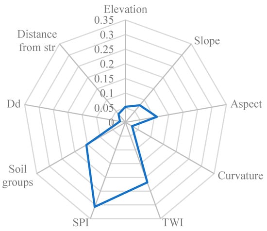
Figure 4.
Weights of factors with AHP method.
When the values of the FR and WoE were examined, it was seen that for values of FR ≥ 0, WoE values might be negative. In order to overcome this problem, WoE-WoEmin was adopted for each condition factor in Step 2 of TOPSIS given in Equation (10). Thus, the FR and WoE values became compatible with each other. Thus, as the values of FR and WoE increase, the flood susceptibility also increases, and all the flood conditioning factors are considered as beneficial. For various distance metrics, the closeness coefficients (Ci) were computed at 25,000 randomly generated points in the Gökırmak watershed. As the Ci values increased, the flood susceptibility throughout the watershed increased. Flood susceptibility maps were generated using various distance metrics by the Krigging interpolation method. Flood susceptibility values were extracted for both training and testing processes for the validation of the predictions.
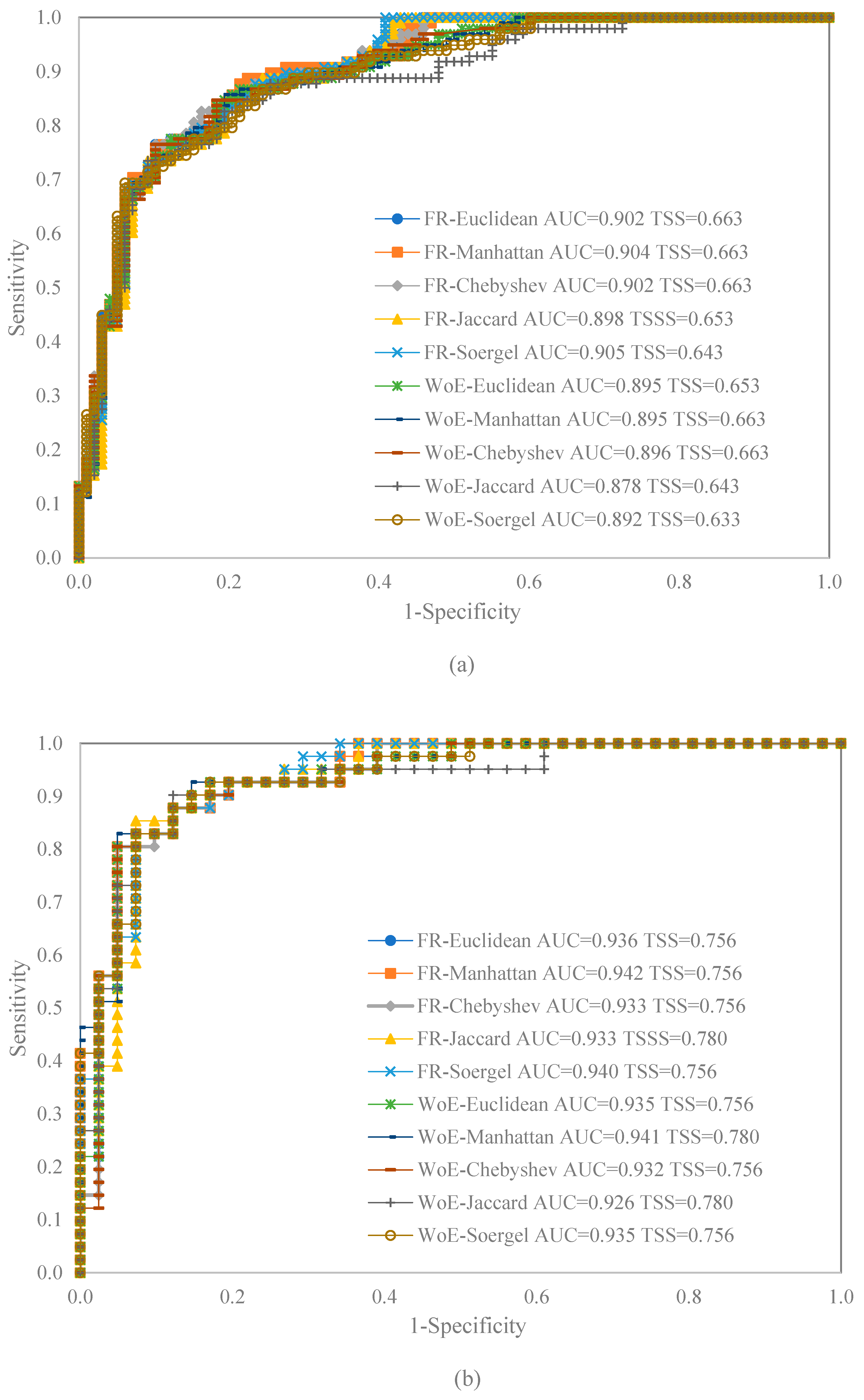
Estimated flood susceptibility maps were validated by the ROC curve method using extracted flood susceptibility values for both training and testing data as given in Figure 5. The AUC values of the training process for FR are 0.898 for Jaccard, 0.902 for Euclidean and Chebyshev, 0.904 for Manhattan, and 0.905 for Soergel while for WoE, they are 0.878 for Jaccard, 0.892 for Soergel, 0.895 for Euclidean and Manhattan, and 0.896 for Chebyshev. The True Skill Statistics (TSS) values for the training process for FR are 0.643 for Soergel, 0.653 for Jaccard, and 0.663 for Euclidean, Chebyshev, and Manhattan whereas for WoE, they are 0.633 for Soergel, 0.643 for Jaccard, 0.653 for Euclidean, and 0.663 for both Manhattan and Chebyshev. The AUC values of the testing process for FR are 0.933 for both Jaccard and Chebyshev, 0.936 for Euclidean, 0.940 for Soergel, and 0.942 for Manhattan while for WoE, they are 0.926 for Jaccard, 0.932 for Chebyshev, 0.935 for Euclidean and Soergel, and 0.941 for Manhattan. For the testing process, the TSS values for FR are 0.756 for all except for Jaccard, which is 0.780. For WoE, they are 0.756 for Euclidean, Chebyshev, and Soergel while they are 0.780 for both Manhattan and Jaccard.
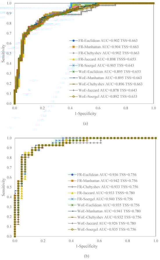
Figure 5.
Validation of estimated flood susceptibility maps by extraction values of (a) training, (b) testing processes.
It was found that the TSS values for both training and testing processes were close since the models estimated the numbers of true/false negative/positive predictions reasonably close to each other. It was noted that the FR results presented very good performance when AUC values were considered. The AUC values obtained by WoE changed in a slightly wider range. Better AUC and TSS values hybridized by both FR and WoE were obtained for the testing process than those in the training process, as seen in Figure 5. However, the trend of obtaining better results by FR was found to continue in both training and testing processes.
The flood susceptibility maps generated by hybridized FR and WoE statistical methods for each distance measure were categorized by classification methods of equal, quantile, natural break (jenks), and geometric intervals in the ArcGIS environment. Figure 6 and Figure 7 show the variations in the percent drainage area of flood susceptibility categories based on the classification algorithms in ArcGIS with distance measure methods hybridized by FR and WoE, respectively. Flood pixels in the classified flood susceptibility potentials were extracted as given in Figure 8 and Figure 9. In accurately estimated flood susceptibility maps, very-low- and low-flood-susceptible pixels are expected to be more than high and very high pixels. Moreover, the flooded points in the classified flood susceptibility maps are expected to be in high and very high categories. The SCAI is the most prominent statistical indicator to put forward this outcome. SCAI is the ratio of values given in Figure 6 to the corresponding values given in Figure 8 for hybridization with FR while for WoE, it is the ratio of values given in Figure 7 and Figure 9 as stated. Akay [21] proposed a power equation to understand the trend of SCAI with regard to the flood potential classes. In the current study, the variations of SCAI values fitted with the flood hazard susceptibility classes were found to be in good agreement with the power equation proposed by Akay [21]. However, the flooded points were not concentrated on very high and high classes, as expected.
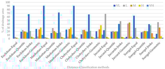
Figure 6.
Variations in percent drainage area of flood susceptibility categories based on equal, quantile, jenks, and geometric intervals with distance measure methods hybridized by FR.
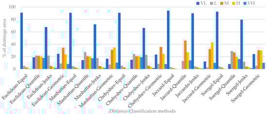
Figure 7.
Variations in percent drainage area of flood susceptibility categories based on equal, quantile, jenks, and geometric intervals with distance measure methods hybridized by WoE.
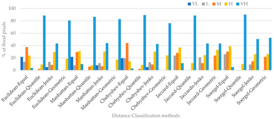
Figure 8.
Variations in percent flood pixels at flood susceptibility categories based on equal, quantile, jenks, and geometric intervals with distance measure methods hybridized by FR.
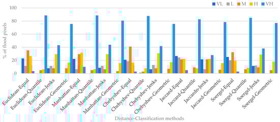
Figure 9.
Variations in percent flood pixels at flood susceptibility categories based on equal, quantile, jenks, and geometric intervals with distance measure methods hybridized by WoE.
Although good results were obtained in some classification methods, results showed that the natural break method gave better predictions on flood hazard susceptibility classes, independent of hybridization methods. It was also noted that good results were obtained when other classification methods were used. Figure 10 and Figure 11 show the classification of the flood susceptibility based on the natural break method for various distance methods and hybridization methods. The Manhattan distance measure calculated by the FR hybridized model gave the best results when compared with other metrics considered. Furthermore, the findings obtained with SCAI also confirmed the results of the ROC analysis.
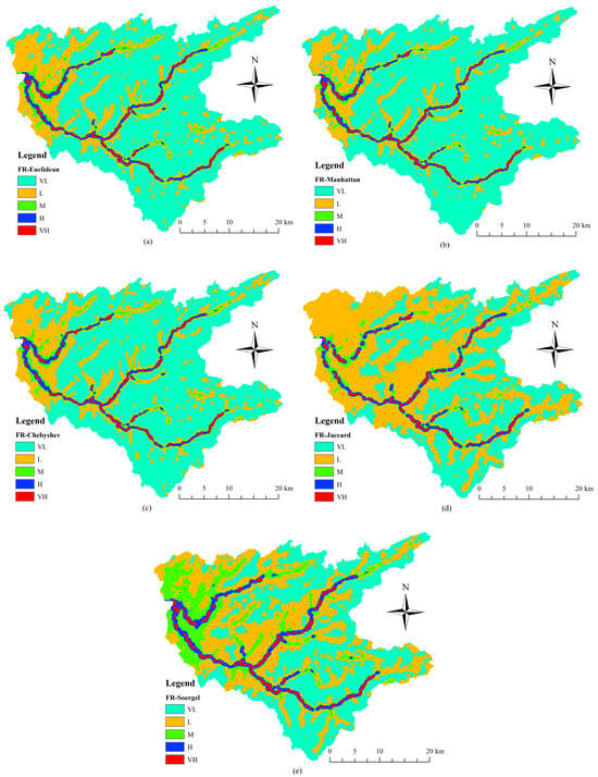
Figure 10.
Flood susceptibility maps processed intervals with distance measure methods hybridized by FR using (a) Euclidean distance, (b) Manhattan distance, (c) Chebyshev distance, (d) Jaccard distance, (e) Soergel distance.
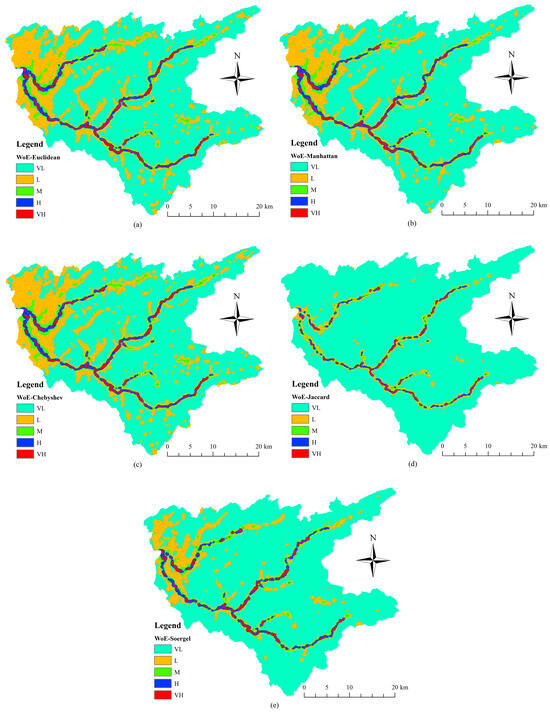
Figure 11.
Flood susceptibility maps processed intervals with distance measure methods hybridized by WoE using (a) Euclidean distance, (b) Manhattan distance, (c) Chebyshev distance, (d) Jaccard distance, (e) Soergel distance.
In this study, the use of various distance measures was adopted to provide a more comprehensive understanding of the underlying dynamics of the TOPSIS method for generating flood susceptibility maps. Model results were sensitive to both hybridization methods and distance measures. In the literature, the Euclidean distance measure is widely used for flood hazard susceptibility mapping studies. However, the results of the current study proved that the Manhattan distance measure might be a better alternative for the studies with improved predictions. Furthermore, the results of Manhattan and Chebyshev distance measures showed that the metrics from the same L1 family as Euclidean gave satisfactory results with no additional computational effort. Since the results of various distance measures altered the generated flood susceptibility maps, the uncertainty induced by using various distance measures may need to be further investigated.
4. Conclusions
In the current study, the effect of hybridization methods and distance measures implemented in the TOPSIS method on the generation of flood hazard susceptibility maps was investigated. A total of 25,000 random points were selected to correspond to approximately 0.2% of the study area in order to sufficiently catch spatial heterogeneities of the flood conditioning factors in the area. The number of random points can be increased to reach a higher percentage in the study area, and thus, results may be slightly improved. However, the results obtained were sufficiently good, so no increment in the number of random points was performed. To achieve the goal of this study, the FR and WoE bivariate statistical methods were used to hybridize the class values of flood conditioning factors. A total of five distance measures, namely Euclidean, Manhattan, Chebyshev, Jaccard, and Soergel, were used. Results showed that the flood hazard susceptibility map is sensitive to the hybridization methods and the distance measures adopted in TOPSIS. In this study, distance measures of the L1 family gave better results according to the validation of estimations, while Manhattan, a distance measure of this family, gave the best results. So, the use of the Euclidean distance measure in TOPSIS, which is widely used in flood hazard susceptibility mapping studies, should be reviewed, and further studies should be conducted to verify that other distance measures might give enhanced results. Furthermore, this study pointed out that there are distance measures and hybridization method-based uncertainties in the predicted results.
Author Contributions
H.A.: Conceptualization, methodology, software, formal analysis, investigation, data curation, writing—review and editing, visualization; M.B.K.: Conceptualization, software, writing—original draft preparation, writing—review and editing, project administration. All authors have read and agreed to the published version of the manuscript.
Funding
Authors acknowledge the financial support of Türkiye Bilimsel ve Teknolojik Araştırma Kurumu, which funded the digital elevation map of the area (Project No. 114M292).
Institutional Review Board Statement
Not applicable.
Informed Consent Statement
Not applicable.
Data Availability Statement
The digital maps and relevant data used in the findings of this study were obtained from the governmental bodies in Türkiye that are not publicly available. So, the data used in this study cannot be made available.
Conflicts of Interest
The authors declare no conflicts of interest.
References
- Gupta, V.; Syed, B.; Pathania, A.; Raaj, S.; Nanda, A.; Awasthi, S.; Shukla, D.P. Hydrometeorological analysis of July-2023 floods in Himachal Pradesh, India. Nat. Hazards 2024, 120, 7549–7574. [Google Scholar] [CrossRef]
- Paliaga, G.; Faccini, F.; Luino, F.; Roccati, A.; Turconi, L. A clustering classification of catchment anthropogenic modification and relationships with floods. Sci. Total Environ. 2020, 740, 139915. [Google Scholar] [CrossRef] [PubMed]
- Razavi, S.; Gober, P.; Maier, H.R.; Brouwer, R.; Wheater, H. Anthropocene flooding: Challenges for science and society. Hydrol. Process. 2020, 34, 1996–2000. [Google Scholar] [CrossRef]
- Rawat, A.; Bisht, M.P.S.; Sundriyal, Y.P.; Banerjee, S.; Singh, V. Assessment of soil erosion, flood risk and groundwater potential of Dhanari watershed using remote sensing and geographic information system, district Uttarkashi, Uttarakhand, India. Appl. Water Sci. 2021, 11, 119. [Google Scholar] [CrossRef]
- Intergovernmental Panel on Climate Change (IPCC). Climate Change 2013: The Physical Science Basis-Contribution of Working Group I to the Fifth Assessment Report of the Intergovernmental Panel on Climate Change; Cambridge University Press: Cambridge, UK; New York, NY, USA, 2013. [Google Scholar]
- Giraldo Osorio, J.D.; Gabriela García Galiano, S. Development of a Sub-Pixel Analysis Method Applied to Dynamic Monitoring of Floods. Int. J. Remote Sens. 2012, 33, 2277–2295. [Google Scholar] [CrossRef]
- Trif, S.; Bilașco, Ș.; Petrea, D.; Roșca, S.; Fodorean, I.; Vescan, I. Spatial modeling through GIS analysis of flood risk and related financial vulnerability: Case study: Turcu River, Romania. Appl. Sci. 2023, 13, 9869. [Google Scholar] [CrossRef]
- Hussein, S.; Abdelkareem, M.; Hussein, R.; Askalany, M. Using remote sensing data for predicting potential areas to flash flood hazards and water resources. Remote Sens. Appl. Soc. Environ. 2019, 16, 100254. [Google Scholar] [CrossRef]
- DeVries, B.; Huang, C.; Armston, J.; Huang, W.; Jones, J.W.; Lang, M.W. Rapid and robust monitoring of flood events using Sentinel-1 and Landsat data on the Google Earth Engine. Remote Sens. Environ. 2020, 240, 111664. [Google Scholar] [CrossRef]
- Ouaba, M.; Saidi, M.E.; Alam, M.J.B. Flood modeling through remote sensing datasets such as LPRM soil moisture and GPM-IMERG precipitation: A case study of ungauged basins across Morocco. Earth Sci. Inform. 2023, 16, 653–674. [Google Scholar] [CrossRef]
- Zoka, M.; Psomiadis, E.; Dercas, N. The Complementary Use of Optical and SAR Data in Monitoring Flood Events and Their Effects. Proceedings 2018, 2, 644. [Google Scholar] [CrossRef]
- Sun, Q.; Nazari, R.; Karimi, M.; Rabbani Fahad, M.G.; Peters, R.W. Comprehensive Flood Risk Assessment for Wastewater Treatment Plants under Extreme Storm Events: A Case Study for New York City, United States. Appl. Sci. 2021, 11, 6694. [Google Scholar] [CrossRef]
- Romali, N.S.; Yusop, Z. Flood damage and risk assessment for urban area in Malaysia. Hydrol. Res. 2021, 52, 142–159. [Google Scholar] [CrossRef]
- Monjardin, C.E.F.; Senoro, D.B.; Magbanlac, J.J.M.; de Jesus, K.L.M.; Tabelin, C.B.; Natal, P.M. Geo-accumulation index of Manganese in soils due to flooding in Boac and Mogpog Rivers, Marinduque, Philippines with mining disaster exposure. Appl. Sci. 2022, 12, 3527. [Google Scholar] [CrossRef]
- Dtissibe, F.Y.; Ari, A.A.A.; Titouna, C.; Thiare, O.; Gueroui, A.M. Flood forecasting based on an artificial neural network scheme. Nat. Hazards 2020, 104, 1211–1237. [Google Scholar] [CrossRef]
- Khoirunisa, N.; Ku, C.Y.; Liu, C.Y. A GIS-based artificial neural network model for flood susceptibility assessment. Int. J. Environ. Res. Public Health 2021, 18, 1072. [Google Scholar] [CrossRef] [PubMed]
- Rehman, N.; Zada, U.; Haleem, K. Quantifying the Influences of Land Use and Rainfall Dynamics on Probable Flood Hazard Zoning. NUST J. Eng. Sci. 2023, 16, 54–68. [Google Scholar] [CrossRef]
- Aghenda, M.; Labbaci, A.; Hssaisoune, M.; Bouchaou, L. Flood susceptibility mapping using neural network based models in Morocco: Case of Souss Watershed (No. EGU24-3447). In Proceedings of the EGU General Assembly 2024, Vienna, Austria, 14–19 April 2024. [Google Scholar] [CrossRef]
- Mashaly, J.; Ghoneim, E. Flash Flood Hazard Using Optical, Radar, and Stereo-Pair Derived DEM: Eastern Desert, Egypt. Remote Sens. 2018, 10, 1204. [Google Scholar] [CrossRef]
- Pal, S.; Saha, A.; Gogoi, P.; Saha, S. An Ensemble of J48 Decision Tree with AdaBoost and Bagging for Flood Susceptibility Mapping in the Sundarbans of West Bengal, India. In Geomorphic Risk Reduction Using Geospatial Methods and Tools. Disaster Risk Reduction; Sarkar, R., Saha, S., Adhikari, B.R., Shaw, R., Eds.; Springer: Singapore, 2024; pp. 117–133. [Google Scholar] [CrossRef]
- Akay, H. Flood susceptibility mapping using information fusion paradigm integrated with decision trees. Water Resour. Manage. 2024, 25, 9325–9346. [Google Scholar] [CrossRef]
- Tehrany, M.S.; Kumar, L.; Jebur, M.N.; Shabani, F. Evaluating the application of the statistical index method in flood susceptibility mapping and its comparison with frequency ratio and logistic regression methods. Geomat. Nat. Hazards Risk. 2018, 10, 79–101. [Google Scholar] [CrossRef]
- Xiong, J.; Li, J.; Cheng, W.; Wang, N.; Guo, L. A GIS-based support vector machine model for flash flood vulnerability assessment and mapping in China. ISPRS Int. J. Geo-Inf. 2019, 8, 297. [Google Scholar] [CrossRef]
- Shikhteymour, S.R.; Borji, M.; Bagheri-Gavkosh, M.; Azimi, E.; Collins, T.W. A novel approach for assessing flood risk with machine learning and multi-criteria decision-making methods. Appl. Geogr. 2023, 158, 103035. [Google Scholar] [CrossRef]
- Rahmati, O.; Pourghasemi, H.R.; Zeinivand, H. Flood susceptibility mapping using frequency ratio and weights-of-evidence models in the Golastan Province, Iran. Geocarto Int. 2016, 31, 42–70. [Google Scholar] [CrossRef]
- Liu, J.; Wang, J.; Xiong, J.; Cheng, W.; Li, Y.; Cao, Y.; He, Y.; Duan, Y.; He, W.; Yang, G. Assessment of flood susceptibility mapping using support vector machine, logistic regression and their ensemble techniques in the Belt and Road region. Geocarto Int. 2022, 37, 9817–9846. [Google Scholar] [CrossRef]
- Pusdekar, P.N.; Dudul, S.V. Flood Susceptibility Mapping and Accuracy Assessment of a River Floodplain Using Bivariate Statistical Methods and AHP Approach. In Proceedings of the 2024 International Conference on Emerging Smart Computing and Informatics (ESCI), Pune, India, 5–7 March 2024; pp. 1–8. [Google Scholar] [CrossRef]
- Samanta, S.; Pal, D.K.; Palsamanta, B. Flood susceptibility analysis through remote sensing, GIS and frequency ratio model. Appl. Water Sci. 2018, 8, 66. [Google Scholar] [CrossRef]
- Saha, S.; Sarkar, D.; Mondal, P. Efficiency exploration of frequency ratio, entropy and weights of evidence-information value models in flood vulnerability assessment: A study of raiganj subdivision, Eastern India. Stoch. Environ. Res. Risk Assess. 2022, 36, 1721–1742. [Google Scholar] [CrossRef]
- Castedo, R.; Isidro, M.L.; Moncoulon, D. Geohazards: Risk Assessment, Mitigation and Prevention; MDPI-Multidisciplinary Digital Publishing Institute: Basel, Switzerland, 2023; p. 608. [Google Scholar] [CrossRef]
- Costache, R.; Pham, Q.B.; Arabameri, A.; Diaconu, D.C.; Costache, I.; Crăciun, A.; Ciobotaru, N.; Pandey, M.; Arora, A.; Ali, S.A.; et al. Flash-flood propagation susceptibility estimation using weights of evidence and their novel ensembles with multicriteria decision-making and machine learning. Geocarto Int. 2022, 37, 8361–8393. [Google Scholar] [CrossRef]
- Sarker, S.C.; Monir, M.M.; Islam, M.N. Analyzing Spatiotemporal Changes in Flood Risk Zones to Mitigate Flood Hazards in a Floodplain Area Using a GIS-Based AHP Technique. In Flood Risk Management; Biswas, B., Ghute, B.B., Eds.; Springer: Singapore, 2024; pp. 23–47. [Google Scholar] [CrossRef]
- Tehrany, M.S.; Kumar, L. The application of a Dempster-Shafer-based evidential belief function in flood susceptibility mapping and comparison with frequency ratio and logistic regression methods. Environ. Earth Sci. 2018, 77, 1–24. [Google Scholar] [CrossRef]
- Muthu, K.; Ramamoorthy, S. Evaluation of urban flood susceptibility through integrated Bivariate statistics and Geospatial technology. Environ. Monit. Assess. 2024, 196, 526. [Google Scholar] [CrossRef] [PubMed]
- Cao, Y.; Jia, H.; Xiong, J.; Cheng, W.; Li, K.; Pang, Q.; Yong, Z. Flash flood susceptibility assessment based on geodetector, certainty factor, and logistic regression analyses in Fujian Province, China. ISPRS Int. J. Geo-Inf. 2020, 9, 748. [Google Scholar] [CrossRef]
- Yuan, X.; Liu, C.; Nie, R.; Yang, Z.; Li, W.; Dai, X.; Cheng, J.; Zhang, J.; Ma, L.; Fu, X.; et al. A comparative analysis of certainty factor-based machine learning methods for collapse and landslide susceptibility mapping in Wenchuan County, China. Remote Sens. 2022, 14, 3259. [Google Scholar] [CrossRef]
- Tu, Y.; Zhao, Y.; Dong, R.; Wang, H.; Ma, Q.; He, B.; Liu, C. Study on Risk Assessment of Flash Floods in Hubei Province. Water 2023, 15, 617. [Google Scholar] [CrossRef]
- Bui, D.T.; Khosravi, K.; Shahabi, H.; Daggupati, P.; Adamowski, J.F.; Melesse, A.M.; Pham, B.T.; Pourghasemi, H.R.; Mahmoudi, M.; Bahrami, S.; et al. Flood spatial modeling in northern Iran using remote sensing and gis: A comparison between evidential belief functions and its ensemble with a multivariate logistic regression model. Remote Sens. 2019, 11, 1589. [Google Scholar] [CrossRef]
- Ivan Ulloa, N.; Chiang, S.H.; Yun, S.H. Flood proxy mapping with normalized difference sigma-naught index and Shannon’s entropy. Remote Sens. 2020, 12, 1384. [Google Scholar] [CrossRef]
- Tehrany, M.S.; Pradhan, B.; Jebur, M.N. Flood susceptibility analysis and its verification using a novel ensemble support vector machine and frequency ratio method. Stoch. Environ. Res. Risk Assess. 2015, 29, 1149–1165. [Google Scholar] [CrossRef]
- Tehrany, M.S.; Pradhan, B.; Mansor, S.; Ahmad, N. Flood susceptibility assessment using GIS-based support vector machine model with different kernel types. Catena 2015, 125, 91–101. [Google Scholar] [CrossRef]
- Costache, R.; Bui, D.T. Identification of areas prone to flash-flood phenomena using multiple-criteria decision-making, bivariate statistics, machine learning, and their ensembles. Sci. Total Environ. 2020, 712, 136492. [Google Scholar] [CrossRef] [PubMed]
- Song, J.Y.; Chung, E.S. Robustness, uncertainty and sensitivity analyses of the TOPSIS method for quantitative climate change vulnerability: A case study of flood damage. Water Resour. Manage. 2016, 30, 4751–4771. [Google Scholar] [CrossRef]
- Rane, N.; Achari, A.; Choudhary, S. Multi-Criteria Decision-Making (MCDM) as a powerful tool for sustainable development: Effective applications of AHP, FAHP, TOPSIS, ELECTRE, and VIKOR in sustainability. Int. Res. J. Modern. Eng. Technol. Sci. 2023, 5, 2654–2670. [Google Scholar] [CrossRef]
- Das, S. Geographic information system and AHP-based flood hazard zonation of Vaitarna basin, Maharashtra, India. Arab. J. Geosci. 2018, 11, 576. [Google Scholar] [CrossRef]
- Roy, S.; Bose, A.; Chowdhury, I.R. Flood risk assessment using geospatial data and multi-criteria decision approach: A study from historically active flood-prone region of Himalayan foothill, India. Arab. J. Geosci. 2021, 14, 1–25. [Google Scholar] [CrossRef]
- Dey, H.; Shao, W.; Haque, M.M.; VanDyke, M. Enhancing Flood Risk Analysis in Harris County: Integrating Flood Susceptibility and Social Vulnerability Mapping. J. Geovis. Spat. Anal. 2024, 8, 19. [Google Scholar] [CrossRef]
- Radwan, F.; Alazba, A.A.; Mossad, A. Flood risk assessment and mapping using AHP in arid and semiarid regions. Acta Geophys. 2019, 67, 215–229. [Google Scholar] [CrossRef]
- Teh Noranis, M.A.; Maslina, Z.; Noraini, C.P. Fuzzy AHP in a knowledge-based framework for early flood warning. In Applied Mechanics and Materials; Trans Tech Publications Ltd.: Zurich, Switzerland, 2019; Volume 892, pp. 143–149. [Google Scholar] [CrossRef]
- Hasanloo, M.; Pahlavani, P.; Bigdeli, B. Flood risk zonation using multi-criteria spatial group fuzzy-AHP decision making and fuzzy overlay analysis. Int. Arch. Photogram. Remote Sens. Spat. Inf. Sci. 2019, 42, 455–460. [Google Scholar] [CrossRef]
- Mitra, R.; Saha, P.; Das, J. Assessment of the performance of GISbased analytical hierarchical process (AHP) approach for flood modelling in Uttar Dinajpur district of West Bengal India. Geomat. Nat. Hazards Risk 2022, 13, 2183–2226. [Google Scholar] [CrossRef]
- Das, S.; Gupta, A. Multi-criteria decision based geospatial mapping of flood susceptibility and temporal hydro-geomorphic changes in the Subarnarekha basin, India. Geosci. Front. 2021, 12, 101206. [Google Scholar] [CrossRef]
- Wang, Y.; Hong, H.; Chen, W.; Li, S.; Pamučar, D.; Gigović, L.; Drobnjak, S.; Bui, D.T.; Duan, H. A hybrid GIS multi-criteria decision-making method for flood susceptibility mapping at Shangyou, China. Remote Sens. 2018, 11, 62. [Google Scholar] [CrossRef]
- Pathan, A.I.; Girish Agnihotri, P.; Said, S.; Patel, D. AHP and TOPSIS based flood risk assessment-a case study of the Navsari City, Gujarat, India. Environ. Monit. Assess. 2022, 194, 509. [Google Scholar] [CrossRef] [PubMed]
- Ameri, A.A.; Pourghasemi, H.R.; Cerda, A. Erodibility prioritization of sub-watersheds using morphometric parameters analysis and its mapping: A comparison among TOPSIS, VIKOR, SAW, and CF multi-criteria decision making models. Sci. Total Environ. 2018, 613, 1385–1400. [Google Scholar] [CrossRef]
- Arabameri, A.; Rezaei, K.; Cerdà, A.; Conoscenti, C.; Kalantari, Z. A comparison of statistical methods and multi-criteria decision making to map flood hazard susceptibility in Northern Iran. Sci. Total Environ. 2019, 660, 443–458. [Google Scholar] [CrossRef]
- Khosravi, K.; Shahabi, H.; Pham, B.T.; Adamowski, J.; Shirzadi, A.; Pradhan, B.; Dou, J.; Ly, H.B.; Gróf, G.; Ho, H.L.; et al. Comparative assessment of flood susceptibility modeling using multi-criteria decision-making analysis and machine learning methods. J. Hydrol. 2019, 573, 311–323. [Google Scholar] [CrossRef]
- Li, J. A Flood Season Division Model Considering Uncertainty and New Information Priority. Water Resour. Manage. 2024, 38, 3755–3784. [Google Scholar] [CrossRef]
- Mitra, R.; Das, J. A comparative assessment of flood susceptibility modelling of GIS-based TOPSIS, VIKOR, and EDAS techniques in the Sub-Himalayan foothills region of Eastern India. Environ. Sci. Pollut. Res. 2023, 30, 16036–16067. [Google Scholar] [CrossRef] [PubMed]
- Karami, M.; Abedi Koupai, J.; Gohari, S.A. Integration of SWAT, SDSM, AHP, and TOPSIS to detect flood-prone areas. Nat. Hazards 2024, 120, 6307–6325. [Google Scholar] [CrossRef]
- Nguyen, H.X.; Nguyen, A.T.; Ngo, A.T.; Phan, V.T.; Nguyen, T.D.; Do, V.T.; Dao, D.C.; Dang, D.T.; Nguyen, A.T.; Nguyen, T.K.; et al. A hybrid approach using GIS-based fuzzy AHP–TOPSIS assessing flood hazards along the south-central coast of Vietnam. Appl. Sci. 2020, 10, 7142. [Google Scholar] [CrossRef]
- Akay, H. Flood hazards susceptibility mapping using statistical, fuzzy logic, and MCDM methods. Soft Comput. 2021, 25, 9325–9346. [Google Scholar] [CrossRef]
- Foroozesh, F.; Monavari, S.M.; Salmanmahiny, A.; Robati, M.; Rahimi, R. Assessment of sustainable urban development based on a hybrid decision-making approach: Group fuzzy BWM, AHP, and TOPSIS–GIS. Sustain. Cities Soc. 2022, 76, 103402. [Google Scholar] [CrossRef]
- Anand, A.K.; Pradhan, S.P. Evaluation of bivariate statistical and hybrid models for the preparation of flood hazard susceptibility maps in the Brahmani River Basin, India. Environ. Earth Sci. 2023, 82, 389. [Google Scholar] [CrossRef]
- Delamaire, A.; Juganaru-Mathieu, M.; Beigbeder, M. Correlation between textual similarity and quality of LDA topic model results. In Proceedings of the 2019 13th International Conference on Research Challenges in Information Science (RCIS), Brussels, Belgium, 29–31 May 2019; pp. 1–6. [Google Scholar] [CrossRef]
- Chen, N.; Chen, L.; Tang, C.; Wu, Z.; Chen, A. Disaster risk evaluation using factor analysis: A case study of Chinese regions. Nat. Hazards 2019, 99, 321–335. [Google Scholar] [CrossRef]
- Axelsson, C.; Giove, S.; Soriani, S. Urban Pluvial Flood Management Part 1: Implementing an AHP-TOPSIS Multi-Criteria Decision Analysis Method for Stakeholder Integration in Urban Climate and Storm Water Adaptation. Water 2021, 13, 2422. [Google Scholar] [CrossRef]
- Rani, M.; Kaushal, S. GeoClust: Feature engineering based framework for location-sensitive disaster event detection using AHP-TOPSIS. Expert Syst. Appl. 2022, 210, 118461. [Google Scholar] [CrossRef]
- Kabak, M.; Saglam, F.; Aktaş, A. Usability analysis of different distance measures on TOPSIS. J. Fac. Eng. Archit. Gazi Univ. 2017, 32, 35–43. [Google Scholar] [CrossRef]
- Kwon, N.; Lee, J.; Park, M.; Yoon, I.; Ahn, Y. Performance Evaluation of Distance Measurement Methods for Construction Noise Prediction Using Case-Based Reasoning. Sustainability 2019, 11, 871. [Google Scholar] [CrossRef]
- Costache, R.; Pham, Q.B.; Sharifi, E.; Linh, N.T.T.; Abba, S.I.; Vojtek, M.; Vojteková, J.; Nhi, P.T.T.; Khoi, D.N. Flash-Flood Susceptibility Assessment Using Multi-Criteria Decision Making and Machine Learning Supported by Remote Sensing and GIS Techniques. Remote Sens. 2020, 12, 106. [Google Scholar] [CrossRef]
- Yanmaz, A.M. Applied Water Resources Engineering; Metu Press: Ankara, Türkiye, 2013. [Google Scholar]
- Alvan Romero, N.; Cigna, F.; Tapete, D. ERS-1/2 and Sentinel-1 SAR Data Mining for Flood Hazard and Risk Assessment in Lima, Peru. Appl. Sci. 2020, 10, 6598. [Google Scholar] [CrossRef]
- Avand, M.; Kuriqi, A.; Khazaei, M.; Ghorbanzadeh, O. DEM resolution effects on machine learning performance for flood probability mapping. J. Hydroenviron. Res. 2022, 40, 1–16. [Google Scholar] [CrossRef]
- Saha, T.K.; Pal, S.; Talukdar, S.; Debanshi, S.; Khatun, R.; Singha, P.; Mandal, I. How far spatial resolution affects the ensemble machine learning-based flood susceptibility prediction in data sparse region. J. Environ. Manage. 2021, 297, 113344. [Google Scholar] [CrossRef]
- Pradhan, B.; Hyun-Joo, O.H.; Buchroithner, M. Weights-of-evidence model applied to landslide susceptibility mapping in a tropical hilly area. Geomat. Nat. Hazards Risk 2010, 1, 199–223. [Google Scholar] [CrossRef]
- Adiat, K.A.N.; Nawawi, M.N.M.; Abdullah, K. Assessing the accuracy of GIS-based elementary multi criteria decision analysis as a spatial prediction tool–a case of predicting potential zones of sustainable groundwater resources. J. Hydrol. 2012, 440–441, 75–89. [Google Scholar] [CrossRef]
- Saaty, T.L. The Analytic Hierarchy Process; McGraw-Hill: New York, NY, USA, 1980. [Google Scholar]
- Hwang, C.L.; Yoon, K. Methods for multiple attribute decision making. In Multiple Attribute Decision Making: Methods and Applications a State-of-the-Art Survey; Springer: Berlin/Heidelberg, Germany, 1981; pp. 58–191. Available online: https://link.springer.com/chapter/10.1007/978-3-642-48318-9_3 (accessed on 2 August 2024).
- Chang, C.H.; Lin, J.J.; Lin, J.H.; Chiang, M.C. Domestic open-end equity mutual fund performance evaluation using extended TOPSIS method with different distance approaches. Expert Sys. Appl. 2010, 37, 4642–4649. [Google Scholar] [CrossRef]
- Chetty, M.; Ngom, A.; Ahmad, S. Pattern Recognition in Bioinformatics; Springer: Berlin/Heidelberg, Germany, 2008. [Google Scholar]
- Yoon, S.; Lee, W. Application of true skill statistics as a practical method for quantitatively assessing CLIMEX performance. Ecol. Indic. 2023, 146, 109830. [Google Scholar] [CrossRef]
- Allouche, O.; Tsoar, A.; Kadmon, R. Assessing the accuracy of species distribution models: Prevalence, kappa and the true skill statistic (TSS). J. Appl. Ecol. 2006, 43, 1223–1232. [Google Scholar] [CrossRef]
- Yesilnacar, E.; Topal, T. Landslide susceptibility mapping: A comparison of logistic regression and neural networks methods in a medium scale study, Hendek region (Turkey). Eng. Geol. 2005, 79, 251–266. [Google Scholar] [CrossRef]


Disclaimer/Publisher’s Note: The statements, opinions and data contained in all publications are solely those of the individual author(s) and contributor(s) and not of MDPI and/or the editor(s). MDPI and/or the editor(s) disclaim responsibility for any injury to people or property resulting from any ideas, methods, instructions or products referred to in the content. |
© 2024 by the authors. Licensee MDPI, Basel, Switzerland. This article is an open access article distributed under the terms and conditions of the Creative Commons Attribution (CC BY) license (https://creativecommons.org/licenses/by/4.0/).