Identifying Elastic Wave Velocity Distribution with Observation Arrival Time Errors Using Weighted Potential Time in Acoustic Emission Tomography

Abstract

Acoustic emission tomography (“AET”) is used to visualize internal structural damage. In this study, we aimed to improve the accuracy of the identified elastic wave velocity distribution when including errors in the observed arrival time, which is used as the observation value in AET. Weights were assigned to the potential excitation times used in location determination and elastic wave velocity distribution according to the magnitude of the potential excitation time and the wave line length. As a result, 100 instances of observation errors were generated for each observation error ratio via truncated normal distribution. The analysis results showed that the normalization error of the elastic wave velocity distribution increased in about 85%, 90%, and 95% of the cases for observation error ratios of 5%, 10%, and 15%, respectively. In conclusion, the weights used for the potential excitation time were effective in identifying elastic wave velocity distribution.

1. Introduction

In recent years, various methods have been used in nondestructive testing (NDT) for evaluating the integrity of existing structures [1,2]. As an NDT technique, acoustic emission testing has been applied to assess the structural soundness of existing structures over the past few decades [3]. AE testing assesses the severity of a damaged area by identifying the distribution of AE source locations. The time difference of arrival (TDOA) method [4,5] has been used as a source location technique. Elastic wave velocity is assumed to be homogenously distributed in the TDOA method, and the source identification equation can be defined using the arrival time difference between two sensors and the ray-path lengths from the sources to the sensors. This technique is widely applied in various fields of health monitoring due to its simple implementation and low computational costs [6,7,8].

However, AEs may not be observed in the severely damaged areas since AEs are generated from the cracks in the structure and the friction between the existing cracks. Therefore, elastic wave tomography has recently been adopted in the literature to investigate structures in their entirety [9]. Elastic wave velocity tomography identifies elastic wave velocity distribution using the first travel times when elastic waves propagate from the excitation position to the attached sensors in the inspection area. It is possible to assess the severity of the structural damage from its velocity distribution since the material’s elastic wave velocity is correlated with its integrity. In practice, however, it is not easy to record the excitation position and time since a sensor must be installed in the vicinity of the excitation location to measure and record these values for every excitation. Thus, identifying the elastic wave velocity distribution may be easier if recording the excitation location and time can be avoided. Acoustic emission tomography (“AET”) was proposed by Schubert to overcome this difficulty [10]. AET is structured via a combination of the source location technique of AE testing and elastic wave tomography and makes it possible to identify the elastic wave velocity distribution even if the excitation location and time are unknown by only using the arrival times of AEs at the sensors. This technique was extended by adopting the ray-trace technique [11,12] and new source localization technique that considers the heterogeneity of elastic wave velocity distribution [13]. As one of the applications, this technique was adopted to visualize the fractures in the rock specimen [14].

Since AET only takes the arrival times as input values, it is not necessary to know the excitation location and time in advance as with elastic wave tomography. Although AET effectively detects structural damage, the resolution of the source locations and the number of sensors in the AET algorithm, cells in the analysis model, and excitations are arbitrary parameters, and the analysis accuracy depends on these parameters. According to Kobayashi et al. [15], a higher source location resolution improves the accuracy of the identified elastic wave velocity distribution. However, these studies have only examined the effect of the source location resolution and rarely those of observation errors.

On the other hand, the accuracy of AE arrival times is crucial for identifying the source location via AE testing and the elastic wave velocity distribution via AET. The Akaike information criterion (AIC) [16] is widely used for detecting the arrival time from the measured waveforms [17,18,19,20]. The boundary between the noise and signal in arrival time detection is defined via the AIC picker and adopted as the arrival time of the measured wave form. However, it is sometimes difficult to clearly define the boundary if the signal to noise ratio (“S/N ratio”) is low. This happens especially if the elastic wave is diffracted from low velocity areas, e.g., a damaged area or void. In this case, the accuracy of the detected arrival time is expected to be lower. Using inaccurate arrival times for source localization degrades the quality of the identified source locations. Consequently, Nakamura et al. proposed a technique that adopts a self-organizing map (SOM) [21] to classify the elastic waves and avoid this issue [17]. SOM is an unsupervised learning method that visualizes data relations and selects the measured waveforms in which the arrival time is accurately detected. By using this technique, it is expected that source localization can be performed without inaccurate arrival times and the source location accuracy would be subsequently improved. In a previous study, artificial AE signals were classified via SOM, and source localization was conducted using a source localization technique based on ray tracing [13] to improve the accuracy of source localization on heterogeneous velocity distributions [22].

As introduced above, the previous challenge was selecting sufficient waveforms that provide accurate arrival times to improve source location accuracy. However, in AET applications, this strategy sometimes causes problems in identifying the elastic wave velocity distribution. Since the diffracted wave yields information about the existing damaged areas, the information is not considered if the wave is omitted. Furthermore, if the sensor and the location of the excitation are close to each other, the first travel time decreases, and the effect of the error on the arrival time is expected to be relatively large. Therefore, past trials have attempted to improve the accuracy of identified elastic wave velocity distribution by removing elastic wave events when the excitations and sensor are closely located to each other. However, these attempts have been performed empirically and have not been theoretically verified. Moreover, there are concerns that reducing the number of ray-paths reduces the number of observation equations in the identification and degrades the accuracy of the identified elastic wave velocity distribution. Therefore, we attempt to improve the identification accuracy of the elastic wave velocity distribution by weighting the observation equations based on the potential excitation times instead of reducing the number of ray-paths. This attempt challenges the effective use of unreliable arrival times by determining its reliability based on the potential excitation times and tries to raise the accuracy of the identified elastic wave velocity distribution as much as possible. The elastic wave velocity distribution is expected to be accurately identified via AET with arrival times observed under undesirable conditions, e.g., severely deteriorated materials or an observation environment with high-level noise, if the attempt is successfully accomplished.

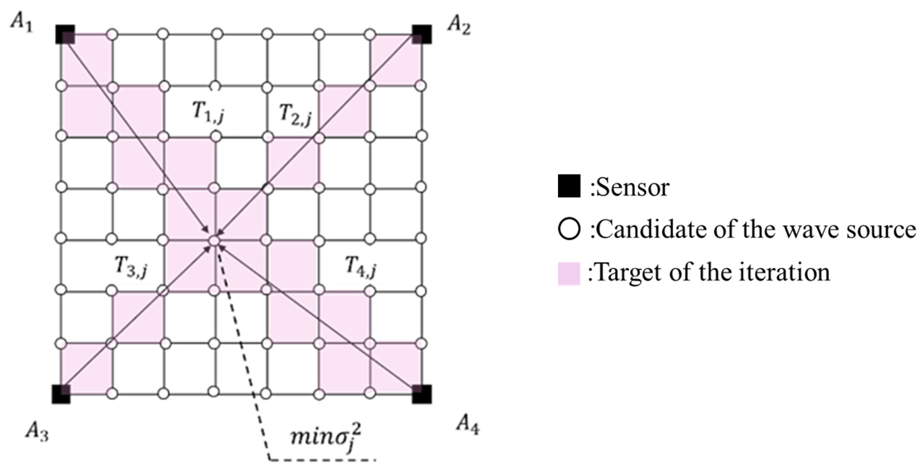
2. Acoustic Emission Tomography

AET is a method developed by combining AE testing and elastic wave tomography, which only uses the AE arrival time at the sensor to locate the excitation source and identify the elastic wave velocity distribution. Generally, the observation equation of AET can be considered as follows.

$$A=f(V,L,O)$$

(1)

where $A$ is the arrival time of the observed elastic wave, $V$ is the elastic wave velocity distribution, $L$ is the position of the AE excitation point, and $O$ is the onset time of the AE. However, practically, AET firstly identifies $O$ and $L$ by assuming $V$ and then identifies $V$ using $O$ and $L$ by combining the source location technique of AE testing and elastic wave velocity tomography [13]. Because AET is constructed on the basis of elastic wave velocity tomography, the first travel time is computed using ray-trace technique in the computational procedure. On the ray-trace technique, the theoretical first travel time $T_{ij}$ is between the source candidate $j$ and the sensor $i$, and the elastic wave velocity distribution is shown in Equation (2).

$$T_{ij}=\sum _k{S}_k{l}_{ijk}$$

(2)

where $S_k$ is slowness, the reciprocal of the elastic wave velocity, in cell k; $l_{ijk}$ is the length of the ray-path from the source candidate $j$ to the sensor $i$ in cell k. Figure 1 shows an overview of the identification of elastic wave velocity distribution via AET. The velocity within each cell in the model is constant. In AET, the elastic wave velocity is updated only on the cells in which the ray-paths pass through. Further, in the least-squares method, the number of ray-paths is the number of equations, and the number of cells is the number of the variables. The number of elastic wave events is a crucial parameter in identifying the elastic wave velocity distribution. Moreover, since the source location is assigned at the nodal and relay points, which are called “candidate points” altogether, in the cell, the number of relay points evidently contributes to the analysis accuracy because it shows the resolution of the source location [22]. On the other hand, the potential excitation time $P_{ij}$ calculated from the arrival time of sensor $i$ at candidate point $j$ is shown in Equation (3).

$$P_{ij}=A_i-T_{ij}$$

(3)

where $A_i$ is the observed arrival time at sensor $i$. It should be noted that the ray-path is approximated as a straight path by assuming the local damage is not severe and the effect of diffraction and refraction is limited in this study. Then, as shown in Figure 1, the elastic wave oscillates in AET; the elastic wave travels in a straight line from the excitation source to the sensor, and the arrival time is used to update the velocity distribution. ${\overline{P}}_j$ is the average of the potential excitation times at candidate point $j$ and it is obtained as shown in Equation (4).

$${\overline{P}}_j={\displaystyle \frac{1}{n}}\sum _{i=0}^n{P}_{ij}$$

(4)

$v_j$ is the variance of the potential excitation times at candidate $j$, which is shown in Equation (5).

$$v_j={\displaystyle \frac{1}{n}}\sum _{i=0}^n(P_{ij}{-\overline{P}}_j{)}^2$$

(5)

where $n$ is the number of sensor points. Although the elastic wave velocity distribution and ray-paths are completely reproduced, the potential excitation times are equal to each other at the source location. However, this is not generally achieved since the reproduction is insufficient due to the limitations of the resolution of modeling. Therefore, the point with the smallest variance of the potential excitation times is selected as the source location and ${\overline{P}}_j$ at the selected point is adopted as the excitation time of the event. After locating the source location, the first travel time can be determined by using ${\overline{P}}_j$. $T_{oij,}$, the first travel time of the elastic wave straightly propagated from the source location to the sensor, is obtained by Equation (6), and $∆T_{ij}$, the residual error of $T_{ij}$ and $T_{oij}$, is computed in Equation (7).

$$T_{oij}=A_i-\overline{P_j}$$

(6)

$$∆T_{ij}=T_{oij}-T_{ij}$$

(7)

Using the least-squares method in which $∆T_{ij}$ of Equation (7) is minimized, the elastic wave velocity distribution is updated until the residual error for the first travel time satisfies the convergence condition. If the amount of correction of slowness in cell k is obtained by the least-squares method as $∆S_k$, the updated slowness in cell k is shown as follows.

$${S_k}^{\left(I\right)}={S_k}^{(I-1)}+∆S_k$$

(8)

where $∆S_k$ is the residual of cell $k$’s slowness, and ${S_k}^{(I-1)}$ is the slowness obtained from the $I-1$ iteration. After updating the elastic wave velocity distribution, the computations of the residual errors of the first travel times are performed on the updated elastic wave velocity distribution on the basis of Equation (7), and then the elastic wave velocity distribution is updated again. This procedure is iteratively conducted until a convergence conduction is achieved.

3. Acoustic Emission Tomography with Potential Excitation Time Weight

When the sensor and excitation points are close to each other and the propagation distance of the elastic wave is short, the first travel time will be small, and the effect of the error on the observed values would be relatively large. Therefore, the identification accuracy of elastic wave velocity distribution is generally improved by removing elastic wave events in which the excitation point is close to the sensor. However, these processes are based on actual measurements and not theoretically validated. Furthermore, the number of excluded equations would increase, resulting in the final number of equations falling short of the number needed to properly identify the elastic wave velocity distribution. In this study, we multiplied the weights via linear interpolation from the potential excitation time distribution and the distances between the candidate points and sensors instead of removing observation equations that may contain large observed arrival time errors.

Considering the weighting of the potential excitation time, the potential excitation time and the distance between the sensor and candidate point in an event are classified into the following three ranges. The ranges that are specified in Equations (9) to Equation (11) are named range 1, range 2 and range 3, respectively.

$$l_{ij}<\beta ,P_{ij}>{\overline{P}}_j$$

(9)

$$l_{ij}>\beta ,P_{ij}>{\overline{P}}_j$$

(10)

$$l_{ij}>\beta ,P_{ij}<{\overline{P}}_j$$

(11)

where $l_{ij}$ is the distance between the sensor $i$ and candidate point $j$, and $\beta$ is the threshold of the distance between the candidate point and sensor for computing the weight. Figure 2a,b show the relation of $l_{ij}$ and $P_{ij}$ without and with weighting.

For determining $\beta$, firstly the line of $P_{ij}$ is equal to ${\overline{P}}_j$, and it is drawn in Figure 2a. Secondly, areas in which the points that represent the pair of $P_{ij}$ and $l_{ij}$ at the candidate points exists are clipped and the boundaries of the clipped areas are computed. Finally, the intersections of the line and the boundaries are calculated, and then minimum distance between the vertical axis and the intersection is adopted as $\beta$. All ranges are divided by these thresholds and are based on elastic wave velocity in the soundness condition and damages condition. In Equation (3), if the ray-path passes through the damage area, $A_i$ is larger than the arrival time of the case in which the ray-path passes through the soundness area because the ray-path diffracts or the travel time is larger. Hence, in accordance with Equation (3), if the location of the candidate point $j$ is identical to the actual source location and the actual ray-path from sensor $i$ to candidate point $j \mathrm{p}\mathrm{a}\mathrm{s}\mathrm{s}\mathrm{e}\mathrm{s}$ through the damage area, $P_{ij}$ would be over ${\overline{P}}_j$. Thus, if $P_{ij}$ is over ${\overline{P}}_j$, it should not be weighted since it involves the information of the damaged area. On the other hand, the potential excitation times of other candidate points that are likely to be affected by errors are weighted so that their absolute values are close to ${\overline{P}}_j$ for clearly identifying damage areas. The potential excitation times in range 3 were processed with weights. $w_{ij}$ is the potential excitation weight from the source candidate $j$ to the sensor $i$, and it is shown in Equation (12).

$$w_{ij}={\displaystyle \frac{l_{ij}-l_{max}}{\beta -l_{max}}}$$

(12)

where $l_{\mathrm{m}\mathrm{a}\mathrm{x}}$ is the maximum length of the ray-path from the source candidate point $j$ to the sensor $i$. ${Pw}_{ij}$ is the potential excitation time of AE with the weight and is shown in Equation (13).

$${Pw}_{ij}={(A}_i-T_{ij})w_{ij}$$

(13)

${\overline{Pw}}_j$ is the average of the potential excitation times with the weight at the candidate point observed at the sensor point and is shown in Equation (14).

$${\overline{Pw}}_j={\displaystyle \frac{1}{\sum _i{w}_{ij}}}\sum _{i=0}^n{P}_{ij}$$

(14)

By using weights for the potential excitation time, the relation f length of the ray-path and potential excitation time from source candidate $j$ to sensor $i$ changes, shown in Figure 2a,b.

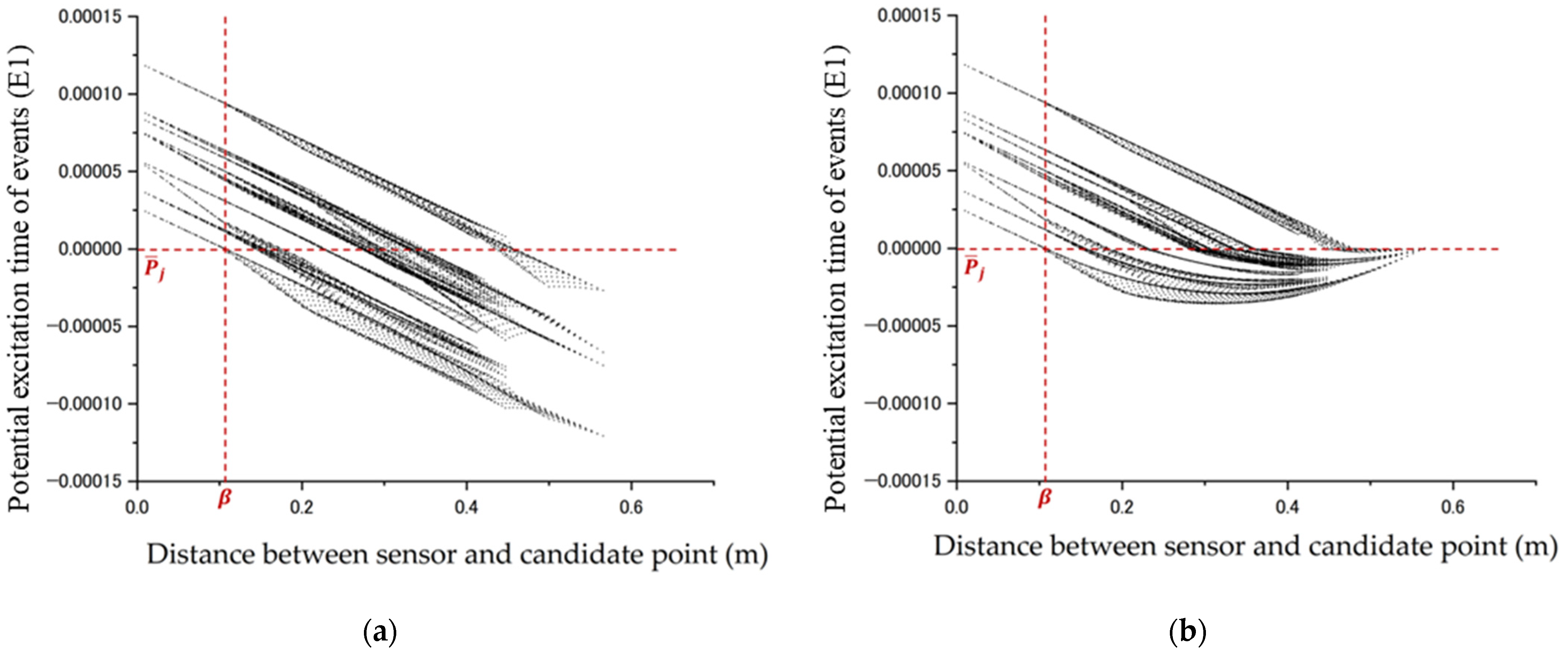
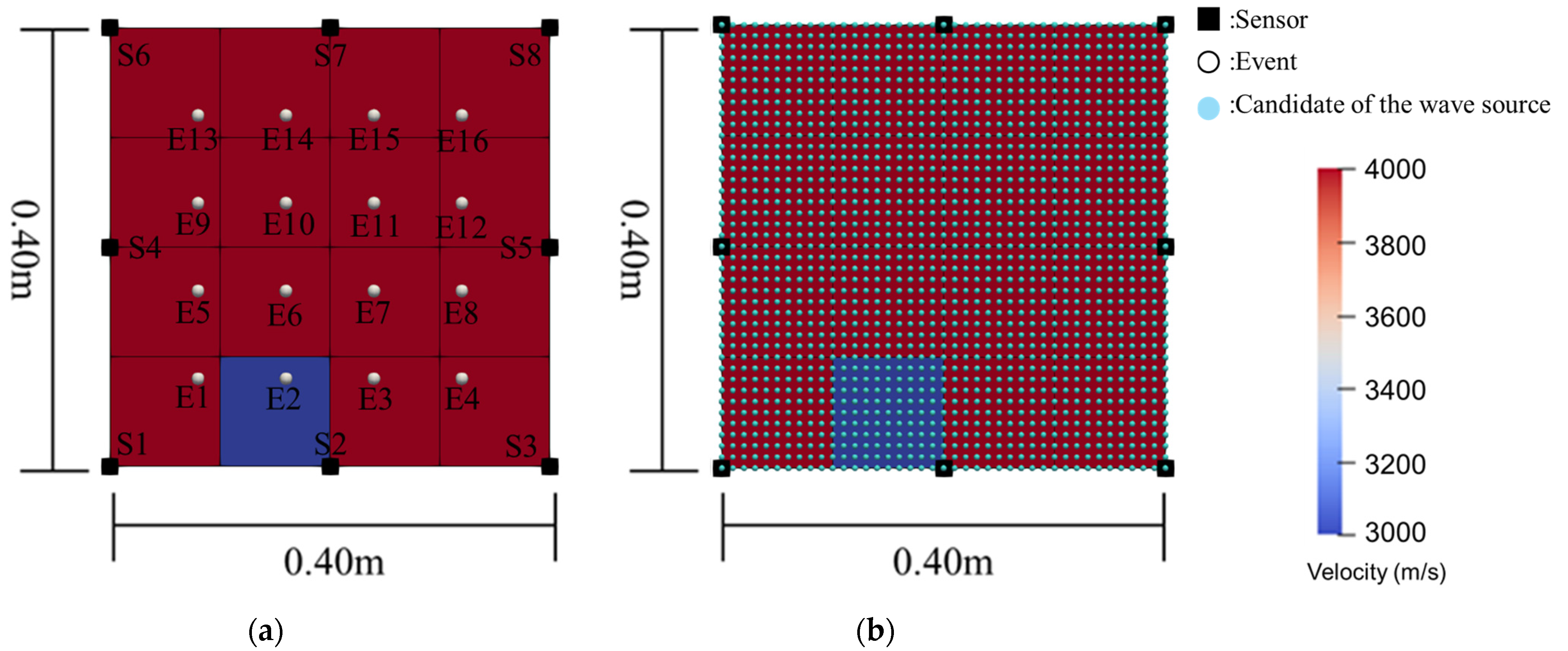
4. Computational Conditions and Generating Arrival Time Observation Errors

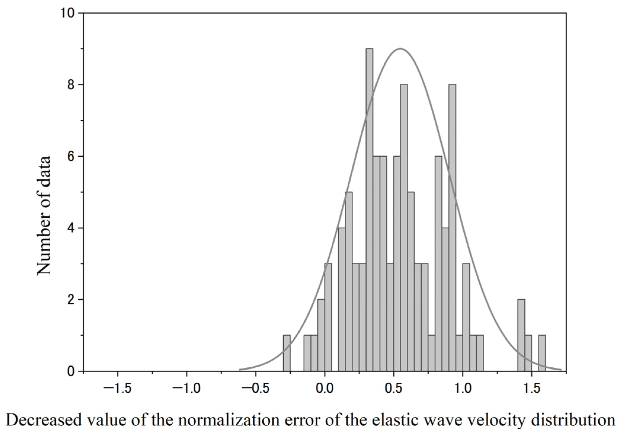
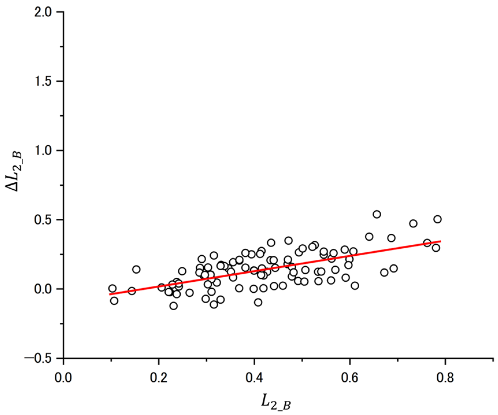
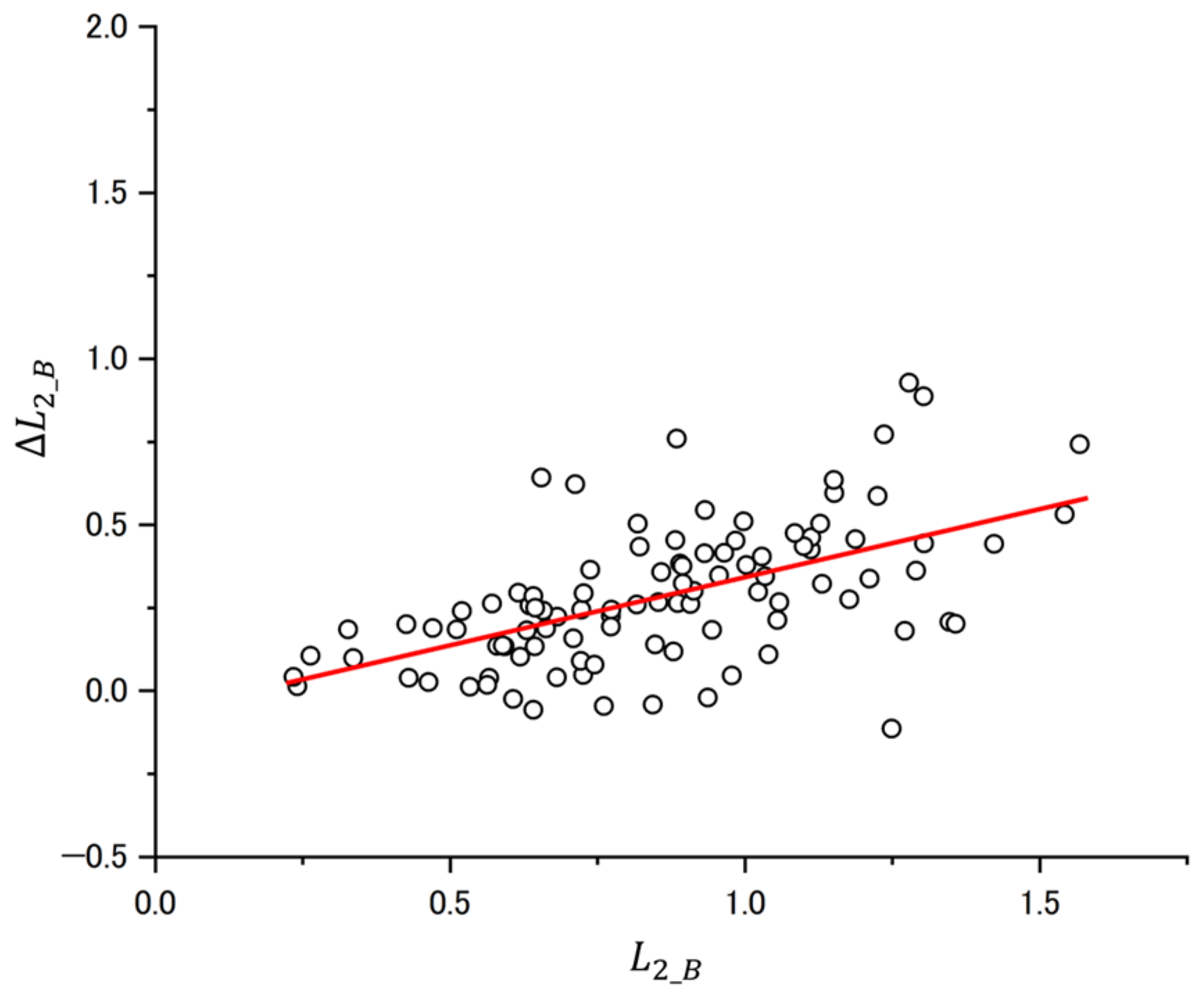
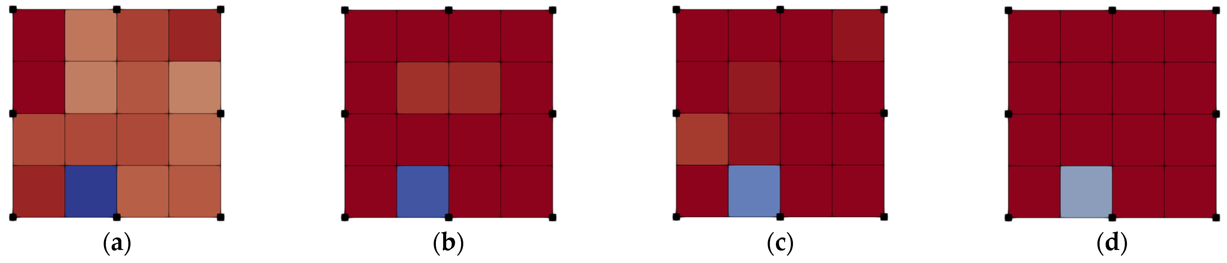
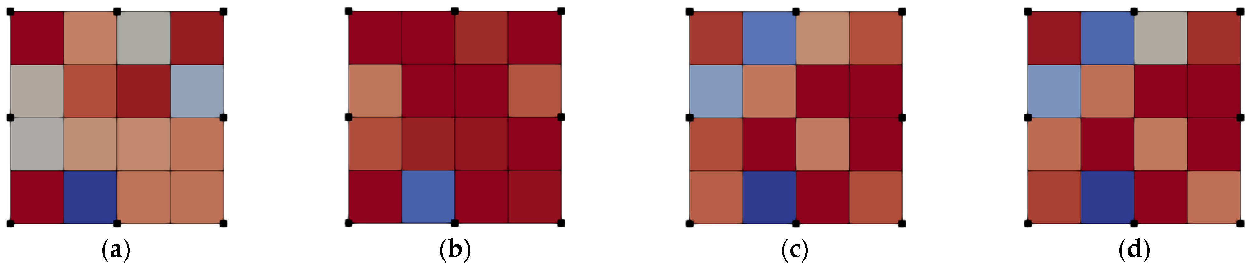
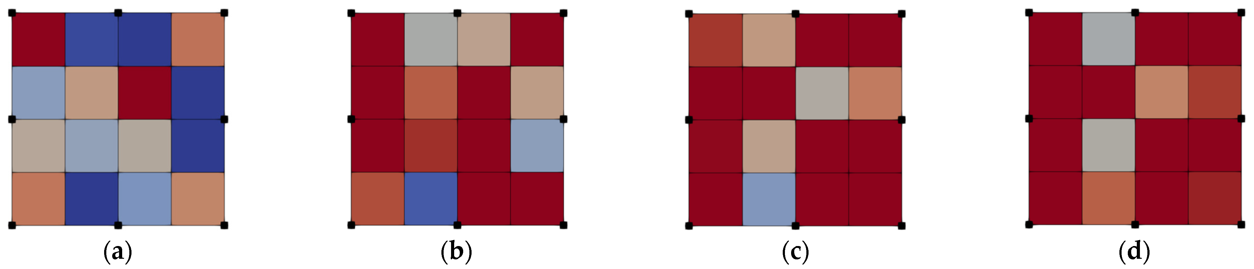
The numerical model that is used for numerical experiments is shown in Figure 3.

Table 1. Numerical model conditions.

Number of elements	16
Number of nodes	25
Model size (m × m)	0.40 × 0.40
Interval of candidate points (cm)	1.0
Elastic wave velocity in soundness condition (m/s)	4000
Damaged part elastic wave velocity (m/s)	3000
Number of events	16
Observation error ratio	0.05~0.15
Number of analyses with different errors at each observed error ratio	100
Number of sensors	8

shows the configuration of the numerical model that is illustrated in Figure 3 and the computational conditions of the numerical experiments. The model simulates a structure in which a local damaged part exists. The model of the analysis area is 0.400 m in both width and height. The sources of the events are installed at 8 cm intervals, and 16 events are generated in total. In addition, eight sensors are installed. One event is defined as the generation of one elastic wave from one source. The black squares in Figure 3 show the sensor location used in the numerical experiments. The observed arrival times are computed by assuming the straight path from the generated sources to the sensors.

Table 2. Locations of installed sensors in the model.

Sensors	x (m)	y (m)
S1	0.0	0.0
S2	0.2	0.0
S3	0.4	0.0
S4	0.0	0.2
S5	0.4	0.2
S6	0.0	0.4
S7	0.2	0.4
S8	0.4	0.4

and

Table 3. Locations of installed events in the model.

Events	x (m)	y (m)
E1	0.08	0.08
E2	0.16	0.08
E3	0.24	0.08
E4	0.32	0.08
E5	0.08	0.16
E6	0.16	0.16
E7	0.24	0.16
E8	0.32	0.16
E9	0.08	0.24
E10	0.16	0.24
E11	0.24	0.24
E12	0.32	0.24
E13	0.08	0.32
E14	0.16	0.32
E15	0.24	0.32
E16	0.32	0.32

show the coordinates of the sensor and source location, respectively. The cell size is 10 cm in height and width. The number of the candidate points is set to 1681, and the number of cells is 16. The initial elastic wave velocity is set to a homogeneous distribution of 4000 m/s, which is that of concrete in the soundness condition.

In this study, the observation error is generated on the basis of truncated normal distribution. Figure 4 is an example of observation arrival time error distribution from the truncated normal distribution that is introduced in Figure 5. It is noteworthy that Figure 5 is created on the basis of the maximum observed arrival time and the error ratio. The mean error value is set to 0 for truncated normal distribution, and the absolute value α of the error generated is obtained from the observation error ratio and the observed maximum arrival time, as shown in Equation (15). The range of the error distribution is from −α to +α. The standard deviation given to the truncated normal distribution is determined separately as described in Equation (16). Random numbers generated in this distribution are used as the observation error values. The total number of random numbers generated is the same as the total number of observed values.

$$\alpha =\pm A_{max}E$$

(15)

$$\sigma ={0.5A}_{max}E$$

(16)

where $A_{max}$ is the maximum value of all observed arrival times to generate errors with a uniform distribution, $E$ is the observation error ratio, and $\sigma$ is the standard deviation of the truncated normal distribution.

5. Results

The normalization errors of the elastic wave velocity distribution and arrival time are defined in Equations (17)–(19). The normalization error of the arrival time are used as convergence conditions of the analysis to visually discriminate between the damaged and healthy areas and numerically judge the results from the normalization error of the elastic wave velocity distribution.

$$L_{2\_A}={\displaystyle \frac{{‖{∆A}_j^c‖}_2}{{‖{∆A}_j^I‖}_2}}$$

(17)

where ${‖{∆A}_j^I‖}_2$ is the sum of the $L_2$ norm based on the observed arrival time from the initial elastic wave velocity distribution obtained for each event $j$, and ${‖{∆A}_j^c‖}_2$ is the sum of the $L_2$ norm based on the observed arrival time from the identified elastic wave velocity distribution obtained for each event $j$. The normalized observation error that is shown in Equation (18) is the ratio of L2 norm of the initial residual error of the arrival times and the residual error of the arrival times at the iteration.

$$L_{2\_B}={\displaystyle \frac{{‖{∆B}_k^c‖}_2}{{‖{∆B}_k^I‖}_2}}$$

(18)

where ${‖{∆B}_k^I‖}_2$ is the sum of the $L_2$ norm of the true and initial elastic wave velocity distributions obtained for each event $j$ at cell k. The normalized error of slowness that is introduced in Equation (18) is the ratio of L2 norm of the difference between the initial slowness distribution and target slowness distribution and L2 norm of the difference between the initial slowness distribution and the slowness distribution at the iteration. Consequently, if the normalized error is smaller, the error is reduced to a greater degree. $∆L_{2\_B}$ are the differences in normalized error of slowness between the unweighted and weighted result.

$$∆L_{2\_B}=L_{2\_B}-L_{2\_B\_w}$$

(19)

where $L_{2\_B\_w}$ is the sum of the $L_2$ norm of the weighted potential excitation times. We investigate the effectiveness of the proposed method that weights the potential excitation time via $∆L_{2\_B}$. It should be noted that $∆L_{2\_B}$ is larger if the proposed method gives better results than the conventional AET. In Figure 6, Figure 7 and Figure 8, 100 instances of observation errors are generated for each observation error ratio via truncated normal distribution. The analysis results show that the normalization errors of the elastic wave velocity distribution increased in about 85%, 90%, and 95% of the cases for observation error ratios of 5%, 10%, and 15%.

Table 4. The normalization error residuals of the identified elastic wave velocity distribution $∆L_{2\_B}$ (weighted and unweighted potential excitation times).

		Residuals of the Normalization Error $∆L_{2\_B}$
		Maximum	Minimum	Average
Observation error ratio E	0.05	0.538152	−0.1221	0.139588
	0.10	0.927147	−0.11333	0.284763
	0.15	1.596866	−0.28338	0.547291

shows the minimum, maximum, and average of $∆L_{2\_B}$ for cases of each observation error ratio. In case of the higher observation error ratio, the maximum and average of $∆L_{2\_B}$ largely increase in accordance with Table 4. This implies that the normalization error of the elastic wave velocity distribution decreases if the observation error ratio increases. However, the minimum of $∆L_{2\_B}$ decreases, which means the accuracy of the identified elastic wave velocity distribution is worse with the proposed technique, in case of the higher observation error ratio.

According to Figure 9, Figure 10 and Figure 11, $∆L_{2\_B}$ increases if $L_{2\_B}$ increases. This reveals that the identified elastic wave velocity distribution is more improved in the presented method if the error of the distribution in the conventional AET is larger. It is also found that the slope is higher in case of a higher observation error ratio.

In Figure 12, Figure 13 and Figure 14, the identified elastic wave velocity distributions are visualized in the conventional AET and the proposed method in the case of the maximum and minimum $∆L_{2\_B}$ with different observation error ratios. In accordance with Figure 12, Figure 13 and Figure 14, it is illustrated that the accuracy of the identified elastic wave velocity distribution is improved in the case of the maximum $∆L_{2\_B}$ in the case of all of the observation error ratios. On the contrary, in the case of the minimum $∆L_{2\_B}$, it seems that the accuracy of the identified elastic wave velocity distribution is improved, although $∆L_{2\_B}$ is negative in 5% of the observation error ratios. This is caused by the difference in the identified elastic wave velocity in the damaged area. In this case, the identified elastic wave velocity distribution in the soundness area, which is colored in red in Figure 3, is closer to the elastic wave velocity in Figure 12d, in comparison with the distribution in Figure 12c. However, the elastic wave velocity in the damaged area, which is colored in blue in Figure 3, is closer to the elastic wave velocity in Figure 12c compared to Figure 12d. Since the difference in the elastic wave velocity in the damaged area is larger than the difference in the soundness area, $∆L_{2\_B}$ becomes negative as a consequence of this, despite the fact that the quality of the contour of the elastic wave velocity distribution is improved. This tendency can be found in cases of maximum $∆L_{2\_B}$ as well. However, the improvement in the elastic wave velocity distribution in the soundness area is larger than the degradation of the elastic wave velocity in the damaged area, and the influence of this is not large, so $∆L_{2\_B}$ and $∆L_{2\_B}$ stay positive. In the case of Figure 14d, the elastic wave velocity in the damaged area is colored in red and the velocity is higher than the one in the soundness area. In this case, it is difficult to distinguish the damaged area. This fact suggests that the proposed method might give worse results in very severe cases if the observed error ratio is extremely high.

6. Discussion

At observation error ratios of 5%, 10%, and 15%, $∆L_{2\_B}$ increases for most of the 100 error patterns, and it means the accuracy of the identified elastic wave velocity distribution is improved in the proposed method. Especially, in cases of the higher observation error ratio, the higher increase rate of $∆L_{2\_B}$ is found in the proposed method in comparison with the conventional AET. However, in the higher observation error ratio, the case with the minimum $∆L_{2\_B}$, it is found that $∆L_{2\_B}$ decreases and the accuracy of the identified elastic wave velocity distribution is decreased. A possible factor is that the standard deviation of the observation error become larger as the observation error ratio increases.

Since the initial elastic wave velocity distribution is specified as a homogeneous one with the elastic wave velocity in the soundness condition, $P_{ij}$ should be larger than the true excitation time. That is why the weight in region 3 is less than 1.0. However, because of the large standard deviation of the observation error, the observed equation that should belong to region 3 may be involved in region 2. This tendency would be more severe if the standard deviation of the observed error is larger. Notably, in the case of the minimum $∆L_{2\_B}$, it is supposed that a large amount of $P_{ij}$ possibly exists in the vicinity of ${\overline{P}}_j$, and the accuracy of the identified elastic wave velocity distribution is decreased as consequence. Furthermore, the higher the observation error ratio, the average value of the potential excitation time ${\overline{P}}_j$—the identified excitation time—is thus different from the true excitation time since $P_{ij}$ involves the error. Because the weight is determined on the basis of ${\overline{P}}_j$, $∆L_{2\_B}$ may decrease even after weighting. Despite the fact that $∆L_{2\_B}$ decreases in the case of minimum $∆L_{2\_B}$, the resultant elastic wave velocity distribution does not change drastically, as illustrated in Figure 12c,d, Figure 13c,d and Figure 14c,d. Thus, we conclude that the proposed method generally improves the accuracy of the identified elastic wave velocity distribution, although $∆L_{2\_B}$ decreases in some cases since the velocity distribution does not change drastically in the cases in which $∆L_{2\_B}$ decreases.

As discussed above, in this study, we could confirm that the proposed method improves the accuracy of the identified elastic wave velocity distribution by performing the numerical investigations.

7. Conclusions

In this study, we proposed a method in which the weight of the observed equation is considered on the basis of the potential excitation time and the distance between the sensor and the candidate point. Based on the results of the numerical investigation, the following conclusions are drawn.

• Reduced normalization errors of the identified elastic wave velocity distribution are observed in most cases by weighting the potential excitation times, including the observation error in arrival times, without reducing the number of observation equations in the proposed method.
• The normalization error of the elastic wave velocity largely decreases as the observation error ratio increases.
• In all of the cases, there is the tendency that the identified elastic wave velocity is improved in the soundness area, while it is degraded in the damaged area.
• In some of the worst cases, the normalization error of the elastic wave velocity distribution is worse. However, its effect is be significant for evaluation of the damage since the change in the distribution is not severe.

In our future studies, we will investigate whether the accuracy of the identified elastic wave velocity distribution is improved by applying the proposed method to arrival times obtained from experiments using concrete specimens with damages.

References

1. Yun, H.D.; Choi, W.C.; Seo, S.Y. Acoustic emission activities and damage evaluation of reinforced concrete beams strengthened with CFRP sheets. NDT E Int. 2010, 43, 615–628. [Google Scholar] [CrossRef]
2. Ciampa, F.; Meo, M. A new algorithm for acoustic emission localization and flexural group velocity determination in anisotropic structures. Compos. Part A Appl. Sci. Manuf. 2010, 41, 1777–1786. [Google Scholar] [CrossRef]
3. Yapar, O.; Basu, P.K.; Volgyesi, P.; Ledeczi, A. Structural health monitoring of bridges with piezoelectric AE sensors. Eng. Fail. Anal. 2015, 56, 150–169. [Google Scholar] [CrossRef]
4. Kawasaki, Y.; Ueda, K.; Izuno, K. AE source location of debonding steel-rod inserted and adhered inside rubber. Constr. Build. Mater. 2021, 279, 122383. [Google Scholar] [CrossRef]
5. Kundu, T. Acoustic source localization. Ultrasonics 2014, 54, 25–38. [Google Scholar] [CrossRef] [PubMed]
6. Huang, J.; Qin, C.Z.; Niu, Y.; Li, R.; Song, Z.; Wang, X. A method for monitoring acoustic emissions in geological media under coupled 3-D stress and fluid flow. J. Pet. Sci. Eng. 2022, 211, 110227. [Google Scholar] [CrossRef]
7. Li, X.; Lin, W.; Mao, W.; Koseki, J. Acoustic emission source location of saturated dense coral sand in triaxial compression tests. In Proceedings of the 8th Japan-China Geotechnical Symposium, Kyoto, Japan, 28–29 September 2020; pp. 14–15. [Google Scholar]
8. Mao, W.; Goto, S.; Towhata, I. A study on particle breakage behavior during pile penetration process using acoustic emission source location. Geosci. Front. 2020, 11, 413–427. [Google Scholar] [CrossRef]
9. Sagradyan, A.; Ogra, N.; Shiotani, T. Application of elastic wave tomography method for damage evaluation in a large-scale reinforced concrete structure. Dev. Built Environ. 2023, 14, 100127. [Google Scholar] [CrossRef]
10. Schubert, F. Basic Principles of Acoustic Emission Tomography. J. Acoust. Emiss. 2004, 22, 147–158. [Google Scholar]
11. Sassa, K.; Ashida, Y.; Kozawa, T.; Yamada, M. Improvement in the accuracy of seismic tomography by use of an effective ray-tracing algorithm. In Proceedings of the MMIJ/IMM Joint Symposium Volume of Papers, Kyoto, Japan, 2–4 October 1989; pp. 129–136. [Google Scholar]
12. Kobayashi, Y. Mesh-independent ray-trace algorithm for concrete structure. Constr. Build. Mater. 2013, 48, 1309–1317. [Google Scholar] [CrossRef]
13. Kobayashi, Y.; Shiotani, T. Innovative AE and NDT Techniques for On-Site Measurement of Concrete and Masonry. In Structures: State-of-the-Art Report of the RILEM Technical Committee 239-MCM, 1st ed.; Ohtsu, M., Ed.; Springer: Dordrecht, The Netherlands, 2016; pp. 47–68. [Google Scholar]
14. Shiotani, T.; Osawa, S.; Kobayashi, Y.; Momoki, S. Application of 3D AE tomography for triaxial tests of rocky specimens. In Proceedings of the 31st Conference of the European Working Group on Acoustic Emission, Dresden, Germany, 3–5 September 2014. [Google Scholar]
15. Kobayashi, Y.; Nakamura, K.; Oda, K. New algorithm of Acoustic Emission Tomography that considers change of emission times of AE events during identification of elastic wave velocity distribution. In Proceedings of the 11th International Conference on Bridge Maintenance, Safety and Management, Barcelona, Spain, 11–15 July 2022. [Google Scholar]
16. Akaike, H. A new look at the statistical model identification. IEEE Trans. Autom. Control 1974, 19, 716–723. [Google Scholar] [CrossRef]
17. Nakamura, K.; Kobayashi, Y.; Oda, K.; Shigemura, S. Classification of Elastic Wave for Non-Destructive Inspections Based on Self-Organizing Map. Sustainability 2023, 15, 4846. [Google Scholar] [CrossRef]
18. Takanami, T.; Kitagawa, G. A new efficient procedure for the estimation of onset times of seismic waves. J. Phys. Earth 1988, 36, 267–290. [Google Scholar] [CrossRef]
19. Sedlak, P.; Hirose, Y.; Enoki, M. Acoustic emission localization in thin multi-layer plates using first-arrival determination. Mech. Syst. Signal Process. 2013, 36, 636–649. [Google Scholar] [CrossRef]
20. Ohno, K.; Ohtsu, M. Crack classification in concrete based on acoustic emission. Constr. Build. Mater. 2010, 24, 2339–2346. [Google Scholar] [CrossRef]
21. Kohonen, T. Essentials of the self-organizing map. Neural Netw. 2013, 37, 52–65. [Google Scholar] [CrossRef] [PubMed]
22. Nakamura, K.; Kobayashi, Y.; Oda, K.; Shigemura, S. Application of Classified Elastic Waves for AE Source Localization Based on Self-Organizing Map. Appl. Sci. 2023, 13, 5745. [Google Scholar] [CrossRef]
Figure 1. Example of elastic wave velocity distribution identification via AET.
Applsci 14 07040 g001
Figure 2. Example of potential excitation time and distance between the sensor and candidate point of event E1 (E = 0.15): (a) non-weight and (b) weight.
Applsci 14 07040 g002
Figure 3. Analysis model schematic of AET: (a) locations of installed events and sensors in the model and (b) locations of installed candidates points in the model.
Applsci 14 07040 g003
Figure 4. Example of observation arrival time error distribution (E = 0.15).
Applsci 14 07040 g004
Figure 5. Example of truncated normal distribution used to generate observation error (E = 0.15).
Applsci 14 07040 g005
Figure 6. Frequency distribution table of the normalization error residuals of the identified elastic wave velocity distribution L 2 _ B (E = 0.05).
Applsci 14 07040 g006
Figure 7. Frequency distribution table of the normalization error residuals of the identified elastic wave velocity distribution L 2 _ B (E = 0.10).
Applsci 14 07040 g007
Figure 8. Frequency distribution table of the normalization error residuals of the identified elastic wave velocity distribution L 2 _ B (E = 0.15).
Applsci 14 07040 g008
Figure 9. Relationship between L 2 _ B and L 2 _ B (red line: regression line between L 2 _ B and L 2 _ B ) (E = 0.05).
Applsci 14 07040 g009
Figure 10. Relationship between L 2 _ B and L 2 _ B (red line: regression line between L 2 _ B and L 2 _ B ) (E = 0.10).
Applsci 14 07040 g010
Figure 11. Relationship between L 2 _ B and L 2 _ B (red line: regression line between L 2 _ B and L 2 _ B ) (E = 0.15).
Applsci 14 07040 g011
Figure 12. Visualization of the identified velocity distribution with observation error ratio (E = 0.05): (a) maximum L 2 _ B and non-weight; (b) maximum L 2 _ B and weight; (c) minimum L 2 _ B and non-weight; and (d) minimum L 2 _ B and weight.
Applsci 14 07040 g012
Figure 13. Visualization of the identified velocity distribution with observation error ratio (E = 0.10): (a) maximum L 2 _ B and non-weight; (b) maximum L 2 _ B and weight; (c) minimum L 2 _ B and non-weight; and (d) minimum L 2 _ B and weight.
Applsci 14 07040 g013
Figure 14. Visualization of the identified velocity distribution with observation error ratio (E = 0.15): (a) maximum L 2 _ B and non-weight; (b) maximum L 2 _ B and weight; (c) minimum L 2 _ B and non-weight; and (d) minimum L 2 _ B and weight.
Applsci 14 07040 g014