Studying the Freezing Law of Reinforcement by Using the Artificial Ground Freezing Method in Shallow Buried Tunnels

Abstract

In this paper, the freezing and strengthening project of the Sanya estuary tunnel is analyzed, which is facilitated by the use of the partial differential equation (PDE) module in COMSOL Multiphysics software. The solid–liquid ratio is utilized as the water–heat coupling term, and the solid mechanics module is introduced to achieve three-field coupling. Numerical simulations are conducted to study changes in the temperature field, moisture field, and vertical displacement due to freezing and expansion in the most unfavorable soil layer during the freezing process. The results indicate that a complete freezing curtain forms around the 30th day. The distribution of freezing pipes significantly influences the freezing effect. The strong freezing zone is characterized by a high cooling rate and rapid water content reduction with the opposite trends being observed in the weak freezing zone. Upon completion of the freezing process, a large uplift of the ground surface is observed with more pronounced vertical displacement changes in areas affected by temperature and phase changes. The maximum vertical displacement of the ground surface deviates from the center position. While the frozen soil curtain meets the design requirements for freezing, the effects of freezing and expansion should be taken into account. These findings could be instrumental in elaborating the most effective freezing and expansion control measures for areas with powdery clay-based layers in AGF-based projects.

1. Introduction

With the continuous expansion of urban development and construction areas, engineering projects that cross rivers, oceans, and other water bodies have become inevitable [1]. This is particularly true for urban highway construction, where large cross-section trans-river tunnels are often employed to traverse such obstacles. Artificial ground freezing technology has emerged as a significant engineering method for underground projects in recent years. This technology’s ability to reinforce soil to facilitate excavation and provide excellent water sealing means it holds substantial engineering value [2,3,4,5]. Artificial ground freezing (AGF) technology utilizes artificial refrigeration techniques, such as brine cycle freezing and liquid nitrogen freezing, to lower the water temperature in a construction soil body [6]. This process transforms the original soil into firm, frozen soil, enhancing its strength and stability and preventing water influx. This technique can form a solid permafrost curtain which supports the safe and efficient construction of underground works [7,8,9,10].

Alzoubi et al. [11,12] conducted indoor experiments on the AGF technique and proposed a novel freezing method. Tounsi et al. [13] used indoor permafrost experimental data to derive a multi-field coupled model in order to ensure that AGF modeling can accurately predict the regular changes in the freezing process. In a practical project, Tounsi et al. [14] used a numerical model to predict the freezing process in a mine tunnel near Cigar Lake, Canada, and analyzed the temperature and displacement data. Auld et al. [15] described the application of AGF technology in tunnel construction and analyzed the effectiveness and versatility of AGF technology through various freezing construction cases. Mauro et al. [6] studied a tunnel freezing project in Naples, Italy, and assessed the heat transfer process of the AGF technique using numerical simulation. In addition, Joudieh et al. [16] carried out a detailed study of the freezing process in soils, studied the effects related to the freezing and expansion of soils, and made several recommendations for the future development of AGF.

The excavation of large-section underwater tunnels often involves the employment of a pipe curtain–permafrost combination structure to provide enclosure during construction. This method utilizes high-strength steel pipe curtains for support. In contrast, forming a permafrost curtain between the pipes effectively seals underground water flow channels, playing a crucial role in water sealing [17,18,19]. The pipe curtain–permafrost combination structure maximizes bearing and water-sealing capabilities, which has led to it being widely used in underwater tunnel construction. A notable example is the construction of the Hong Kong–Zhuhai–Macao Bridge Gongbei Tunnel, where the successful application of the pipe curtain–permafrost combination structure has significantly advanced the technology. This success has not only enhanced the application scope of the pipe curtain–permafrost combination structure but also led to the development of a new pipe curtain freezing construction technology [20,21,22,23].

In addition, the soil experiences freezing and expansion effects during the soil freezing process. This process includes in situ freezing and expansion as well as sub-condensation freezing and expansion. The former refers to the conversion of liquid water within the closed pores of the soil into ice. The latter involves the migration of free liquid water within the pores, driven by the temperature gradient difference during the freezing process, which subsequently transforms into ice, causing volume expansion. Reviewing relevant information and previous research shows that the freezing expansion caused by in situ freezing has a comparatively smaller effect than that caused by sub-condensation freezing and expansion. Therefore, soil freezing expansion should be considered from a multi-field coupling perspective [24,25,26,27].

A shallow buried tunnel project in Sanya, which is part of a highway crossing at the mouth of a large cross-section tunnel, employs a new pipe curtain method for tunnel enclosure construction. This method relies on freezing technology to reinforce the surrounding soil. A stable permafrost curtain is established upon starting the freezing process, which is crucial for subsequent construction activities, such as pipe cutting, welding, pouring, and excavation. Ensuring the conditions for constructing the freezing curtain is vital for the success of these subsequent processes. The project’s preliminary design necessitates using many freezing pipes, as the soil primarily consists of a high water content clay layer. The low temperatures sustained during the freezing process will cause the pore water in the soil to undergo phase change and migration. Consequently, while the soil is being reinforced, the effects of frost heave should not be underestimated.

In recent years, with the rapid development and widespread application of computer technology, numerical calculation methods have become a powerful means of solving most engineering problems [28]. Consequently, this paper focuses on the secondary development of the Partial Differential Equation (PDE) module in COMSOL software (COMSOL Multiphysics 6.0) to achieve full coupling of the hydrothermal physical field. Additionally, the successive solution and sequential coupling of the displacement field are utilized to establish a three-dimensional numerical model of the horizontal freezing reinforcement for the starting section of the Sanya Estuary Passage Tunnel Project. A typical parameter analysis is conducted to study the distribution of the freezing temperature field, the moisture field, and the characteristic pattern of the displacement field. This analysis provides a basis for optimizing the freezing design of this project and similar projects. By examining these parameters, a comprehensive understanding of the freezing process can be achieved, facilitating improvements in the efficiency and effectiveness of freezing designs in future engineering endeavors.

2. Project Overview

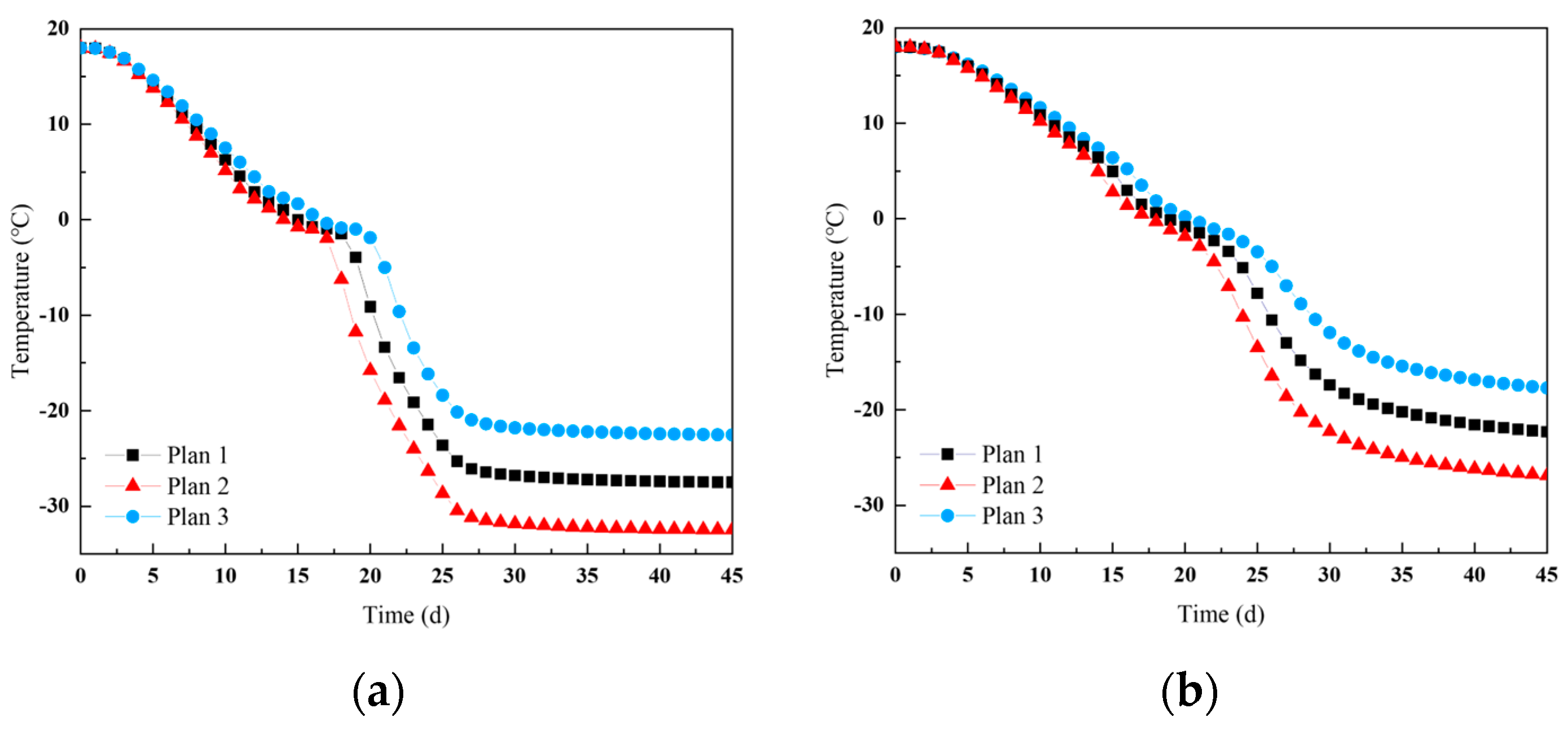
2.1. Project Profile

The tunnel freeze reinforcement project in Tianya District, Sanya City, spans the Sanya River estuary, linking the north bank of the Hexi area with the south bank of the Luhuitou Peninsula. This project serves as a critical conduit connecting the Luhuitou Peninsula and is significant for supporting the development of the southern sea area of the headquarters economy. Additionally, it plays a pivotal role in refining the city’s road network, enhancing regional traffic accessibility, eliminating traffic bottlenecks, and alleviating transit traffic pressure in the old city. The project features upper and lower stacked tunnels like the Gongbei Tunnel, totaling 3118 m. The soil layers encountered are complex and diverse, including miscellaneous fill, pulverized clay, coral clasts, strongly weathered quartz sandstone, moderately weathered quartz sandstone, and fine sand. The main construction soil is characterized by its strongly permeable layer.

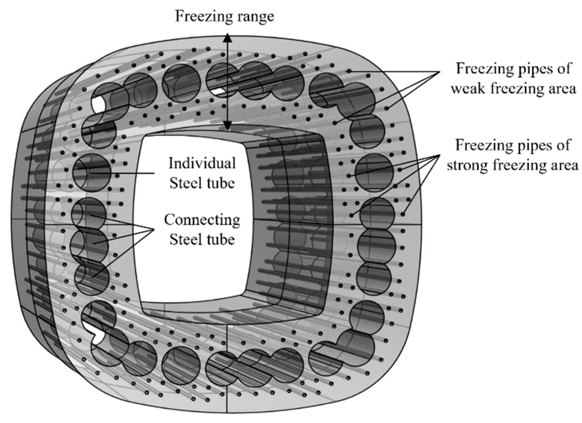
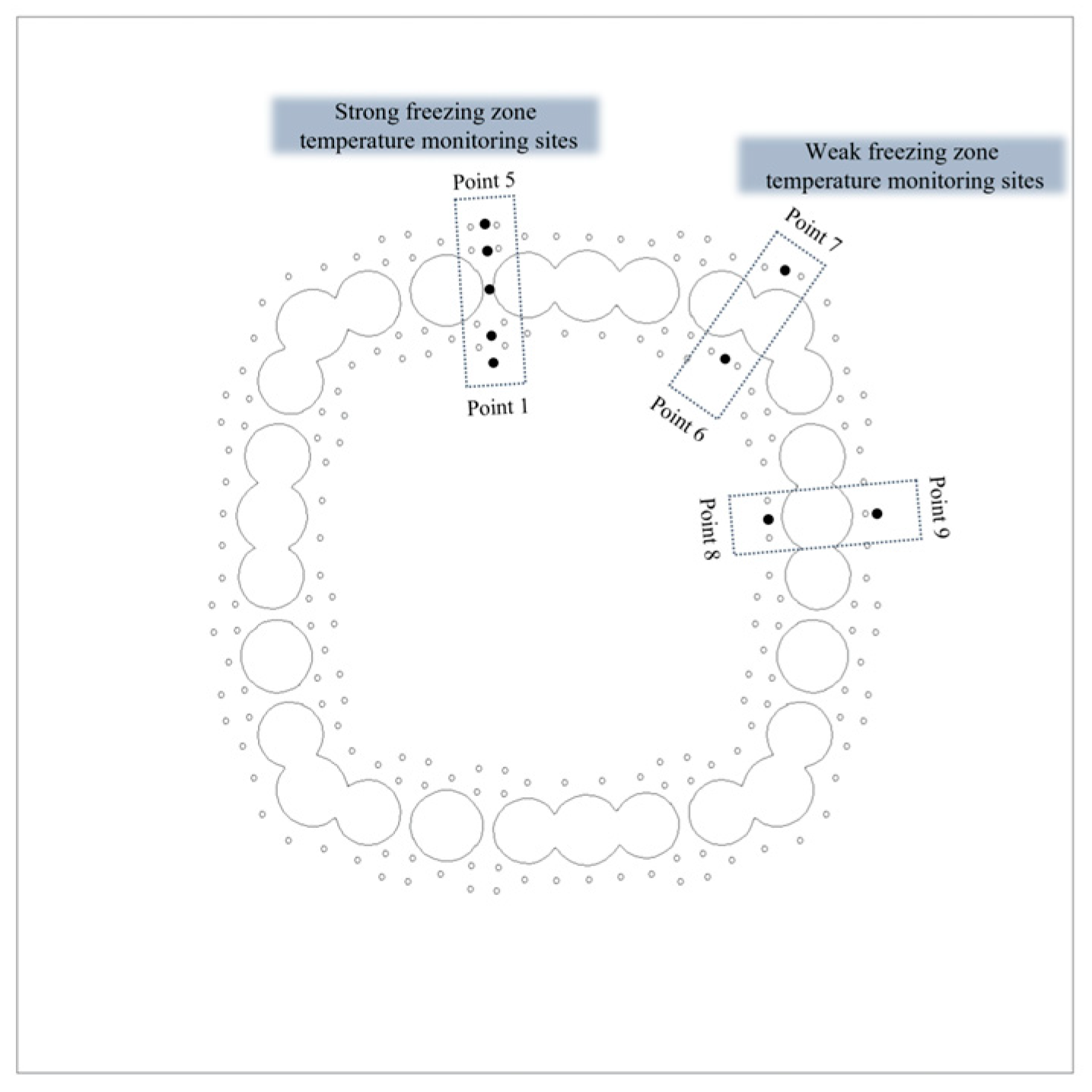
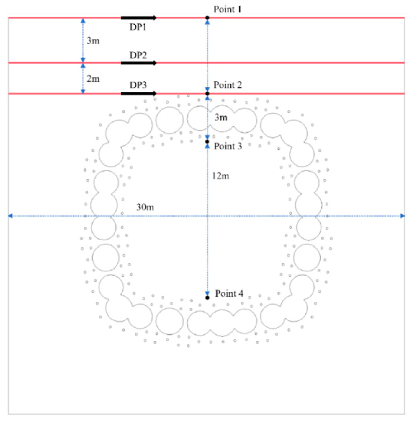
2.2. Freeze Pipe Arrangement

The freezing pipes selected for this project are φ108 mm × 10 mm. There is a total of 176 pipes arranged in two layers in the ring direction. Overall, 96 freezing pipes are installed in the outer ring, while the inner ring consists of 80 freezing pipes. The freezing area is divided into strong and weak freezing zones. The pipes are spaced 800 mm apart in the strong freezing zone, whereas in the weak freezing zone, the spacing is 950 mm. The pipe curtain in the strong freezing zone is configured with a single steel pipe topping, and in the weak freezing zone, it is arranged with three occluded steel jacking pipes. This ring arrangement includes 28 steel pipes, comprising eight groups of occluded steel pipes and 4 independent steel pipes. Upon completion of the freezing process, the steel pipes are cut and connected using steel plate welding to form the pipe curtain. The cut steel pipes are supported by freezing, and together with the freezing curtain, they serve the dual purpose of water sealing and structural support. The arrangement of the freezing and jacking steel pipes is illustrated in Figure 1.

3. Numerical Simulation

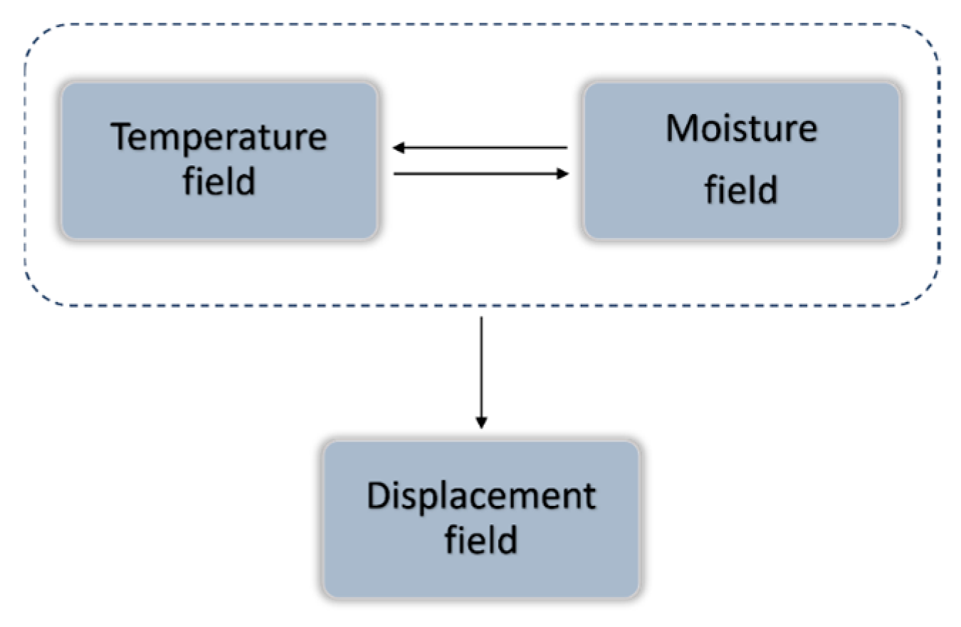
3.1. Governing Equation

3.1.1. Temperature Field Control Equation

Considering the three-dimensional hydrothermal coupling problem, the differential equation for heat transfer in permafrost, as derived from Fourier’s law, is as follows:

$$\rho C\left(\theta \right){\displaystyle \frac{\partial T}{\partial t}}=\lambda \left(\theta \right){𝛻}^{2}T+L\cdot {\rho }_I{\displaystyle \frac{\partial {\theta }_I}{\partial t}}$$

(1)

where $\rho$ is the weighted density of the soil, $C$ is the specific heat capacity, $T$ is the temperature, $\lambda$ is the thermal conductivity, $L$ is the latent heat of the water–ice phase change, and ${\theta }_I$ is the volumetric ice content.

3.1.2. Moisture Field Control Equation

The migration of unfrozen water in permafrost obeys Darcy’s law. According to Richard’s equation and considering the blocking effect of pore ice on the migration of unfrozen water during the frozen ice–water phase transition, the governing equation for water in permafrost is as follows:

$${\displaystyle \frac{\partial {\theta }_u}{\partial t}}+{\displaystyle \frac{{\rho }_I}{{\rho }_w}}{\displaystyle \frac{\partial {\theta }_I}{\partial t}}=𝛻\left[D\left({\theta }_u\right)𝛻{\theta }_u+k\left({\theta }_u\right)\right]$$

(2)

where ${\theta }_u$ is the volumetric water content, ${\rho }_I$ is the ice density, ${\rho }_w$ is the water density, $D$ is the diffusion coefficient, and $k$ is the permeability coefficient.

In the above equation, the diffusivity of water in permafrost is calculated as follows:

$$D\left({\theta }_u\right)={\displaystyle \frac{k\left({\theta }_u\right)}{c\left({\theta }_u\right)}}\cdot I$$

(3)

where $k\left({\theta }_u\right)$ is the permeability of the soil, $c\left({\theta }_u\right)$ is the specific water capacity, and $I$ is the impedance factor [29], which is meant to describe the hindrance of water migration by the ice in the soil, and it is obtained via the following:

$$I=10^{-10{\theta }_i}$$

(4)

$k\left({\theta }_u\right)$ is calculated using the following equation:

$$k\left({\theta }_u\right)=k_s\cdot S^l{\left(1-{\left(1-S^{{\displaystyle \frac{1}{m}}}\right)}^m\right)}^2$$

(5)

$c\left({\theta }_u\right)$ is calculated using the following equation:

$$c\left({\theta }_u\right)={\displaystyle \frac{a_{0}m}{1-m}}\cdot \left({\theta }_s-{\theta }_r\right)\cdot S^{{\displaystyle \frac{1}{m}}}{\left(1-S^{{\displaystyle \frac{1}{m}}}\right)}^m$$

(6)

where $k_s$ is the coefficient of permeability of saturated soil; $S$ is the relative saturation; and $a_0$, $m$, and $l$ are intrinsic parameters that vary with the soil.

Since volumetric water content and ice content variables exist between the heat transfer and water migration equations and the number of equations is less than the number of unknown variables, a coupling term must be introduced to link the hydrothermal equations. The solid–liquid ratio $B\left(T\right)$ is invoked as this coupling term [30], which expresses the ratio of the volume of pore ice in the permafrost to that in the unfrozen soil. The calculation formula is as follows:

$$B_I={\displaystyle \frac{{\theta }_i}{{\theta }_u}}=\left\{\begin{array}{ccc}1.1{\left({\displaystyle \frac{T}{T_f}}\right)}^B& -1& T<T_f\\ 0& & T\ge T_f\end{array}\right.$$

(7)

where $T_f$ is the soil’s freezing temperature, and $B$ is a constant that varies with soil quality and salt content.

Based on the Van Genuchten (VG) stagnant water model, the relative saturation S of permafrost is defined as follows:

$$S={\displaystyle \frac{{\theta }_u-{\theta }_r}{{\theta }_s-{\theta }_r}}$$

(8)

where ${\theta }_r$ is the residual water content, and ${\theta }_s$ is the saturated water content [31,32].

3.1.3. Hydrothermal Coupling PDE Secondary Development Module

The introduction of the coefficient-based Partial Differential Equations (PDE) module in COMSOL allows for secondary development by inputting the various coefficients in the form of the following equations:

$$e_a{\displaystyle \frac{{\partial }^{2}T}{\partial t^2}}+d_a{\displaystyle \frac{\partial T}{\partial t}}+𝛻\cdot \left(-c𝛻T-\alpha T+\gamma \right)+\beta \cdot 𝛻T+aT=f$$

(9)

By deforming the temperature field control equation and comparing it with the above equation, the coefficients of each of the temperature field equations can be derived as follows:

$$\left\{\begin{array}{c}{d}_a=\rho C\left(\theta \right)-L\cdot {\rho }_I\cdot \left[\left({\theta }_s-{\theta }_r\right)\cdot S+{\theta }_r\right]\cdot {\displaystyle \frac{\partial B\left(T\right)}{\partial T}}\\ c=\lambda \left(\theta \right)\\ f=L{\rho }_I\cdot \left({\theta }_s-{\theta }_r\right)\cdot B\left(T\right)\cdot {\displaystyle \frac{\partial S}{\partial t}}\end{array}\right.$$

(10)

By deforming the moisture field control equation and comparing it with the above equation, the coefficients of each of the moisture field equations can be derived as follows:

$$\left\{\begin{array}{c}{d}_a=1+{\displaystyle \frac{{\rho }_I}{{\rho }_w}}B\left(T\right)\\ c=D\left(S\right)\\ \gamma =-K\left(S\right)\\ a={\displaystyle \frac{{\rho }_I}{{\rho }_w}}\cdot {\displaystyle \frac{\partial B\left(T\right)}{\partial t}}\end{array}\right.$$

(11)

3.1.4. Displacement Field Control Equation

As illustrated in Figure 2, considering the reliability of the model calculation and the need to simplify the calculation speed, this study simplifies the hydrothermal three-field coupling relationship [33,34]. Specifically, the full coupling of hydrothermal processes is considered first, which is followed by sequential unidirectional coupling through the inheritance of the solution. The corresponding control equation is as follows:

$${\epsilon }_{vf}={\theta }_i+{\theta }_u-n$$

(12)

$$\begin{array}{c}{\epsilon }_{vT}=3\left[{\beta }_s{\theta }_s\left(T-T_0\right)+{\beta }_u{\theta }_u\left(T-T_0\right)+{\beta }_i{\theta }_i\left(T-T_f\right)\right]\end{array}$$

(13)

where ${\epsilon }_{vf}$ is the volumetric strain due to the ice–water phase transition, n is the initial porosity; ${\epsilon }_{vT}$ is the volumetric strain due to temperature change, and ${\beta }_s$, ${\beta }_u$, and ${\beta }_i$ are the coefficients of linear expansion for the soil particles, unfrozen water, and ice, respectively.

3.2. Numerical Modeling Assumptions

Based on the actual engineering profile and model calculation theory, the following assumptions are made for the hydrothermal coupling model of this freezing project:

(1)

The investigation report for this project indicates that powdery clay with high water content produces a large freezing rate during the freezing process. Therefore, this study simplifies the soil body to a homogeneous, continuous, isotropic, and linearly elastic soil layer with the most unfavorable soil parameters. Each parameter is derived from weighted values based on the investigation report, and the soil body has an initial temperature of 18 °C.

(2)

Based on existing research [35], it is assumed that the soil body begins to freeze at −1 °C and forms a stable permafrost structure at −10 °C.

(3)

Neglecting the loss of cold during the brine circulation process and the influence of heat convection and radiation during heat transfer, the brine temperature is directly applied to the wall of the freezing pipe as a temperature load with heat transferred solely by conduction.

(4)

It is assumed that moisture migration in the soil conforms to Darcy’s law.

(5)

The migration of salts and other solutes in the soil is not considered. Water migration is assumed to occur primarily in liquid form, ignoring the movement of gaseous water. The soil is considered saturated, containing only liquid water and solid ice in the pore space, with the saturated water content equating to the soil’s porosity.

(6)

It is assumed that ice crystals and the solid phase of the soil are incompressible.

3.3. Numerical Modeling

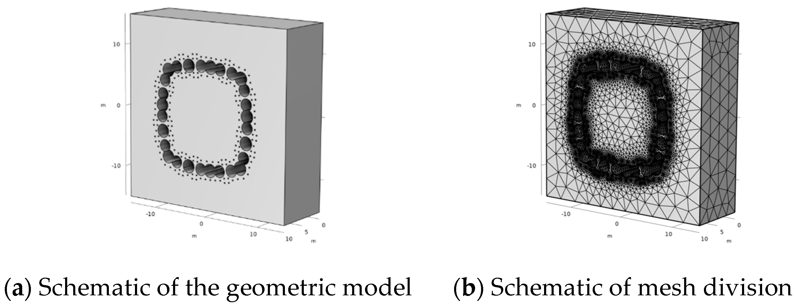
3.3.1. Geometric Modeling, Meshing and Boundary Conditions

A three-dimensional finite element model is established according to the project’s actual burial depth, the boundary error induced by the freezing wall’s influence range, and the complexity of the model calculation. The freezing pipe has dimensions of φ108 mm × 10 mm, and a size model with dimensions of 30 m × 10 m × 30 m is selected for the calculation.

The numerical model calculation adopts a user-defined free tetrahedral grid with an adaptive mode. The mesh size around the freezing pipe is reduced to reduce calculation error and improve convergence. The mesh size can be appropriately increased in the boundary region, where the temperature change due to the freezing pipe is not directly affected. This approach ensures a reasonable division of the mesh density. The numerical model ultimately consists of 216,339 cells.

The initial temperature of the model is set to the actual working temperature, which corresponds to the original ground temperature of the actual working condition, i.e., 18 °C. The initial condition of the moisture field is set to saturation S = 1 and combined with the test parameters of the most unfavorable soil layer in the working condition; the initial water content is set at 40%. To closely mimic the working conditions, gravitational acceleration is set to g. The boundaries around the model are adiabatic and have a constant temperature, while the cooling plan defines the boundary conditions at the freezing pipe. The boundaries around the moisture field are set as zero flux boundaries, considering internal migration. The bottom boundary is a fixed-displacement boundary, and the normal displacement is constrained all around, as shown in Figure 3.

3.3.2. Selection of Relevant Parameters

Based on the engineering design scheme, the investigation report, and previous research [36], the parameters for each model calculation and the brine cooling plan were obtained, as shown in

Table 1. Calculation parameters for the most unfavorable soil layer.

Type of Parameter	Parameter	Value
Soil thermophysical parameters	Soil density (kg/m3)	1930
	Water density (kg/m3)	1000
	Ice density (kg/m3)	920
	Thermal conductivity of soil (W/(m·°C))	1.22
	Thermal conductivity of water (W/(m·°C))	0.63
	Thermal conductivity of ice (W/(m·°C))	2.31
	Specific heat capacity of soil (J/(kg·°C))	1530
	Specific heat capacity of water (J/(kg·°C))	4200
	Specific heat capacity of ice (J/(kg·°C))	2100
	Latent heat of phase transition (J/kg)	334,720
Soil mechanical parameters	Elastic modulus of unfrozen soil (MPa)	40
	Elastic modulus of frozen soil (MPa)	120
	Unfrozen ground cohesion (kPa)	30
	Angle of internal friction in unfrozen soil (°)	22
	Poisson’s ratio for unfrozen soil	0.31
	Poisson’s ratio for frozen soil	0.23

and

Table 2. Brine cycle freezing tube cooling program.

Time/d	0	10	20	30	45
Temperature/°C	18	0	−20	−28	−28

.

4. Analysis of Simulation Results

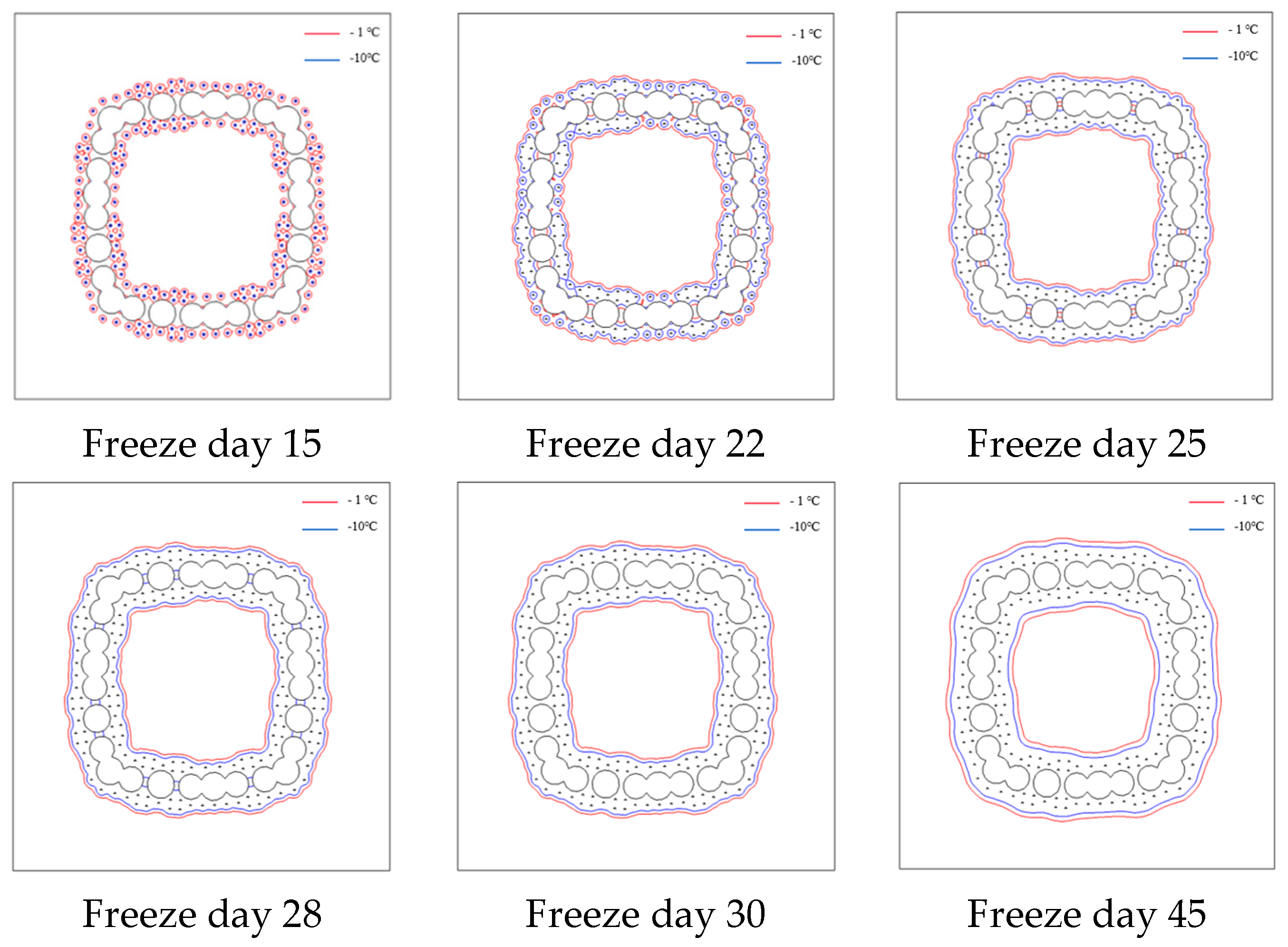
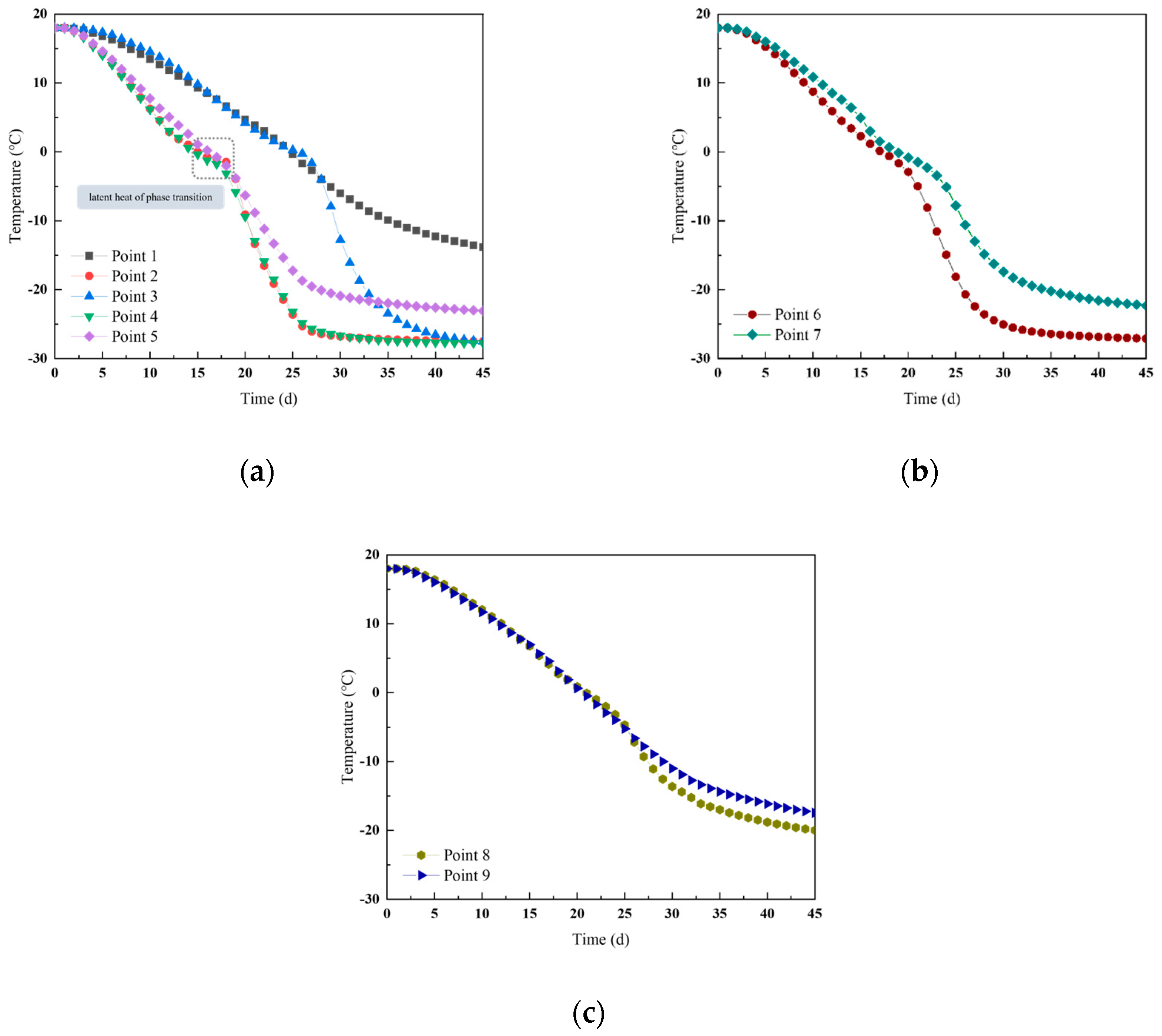
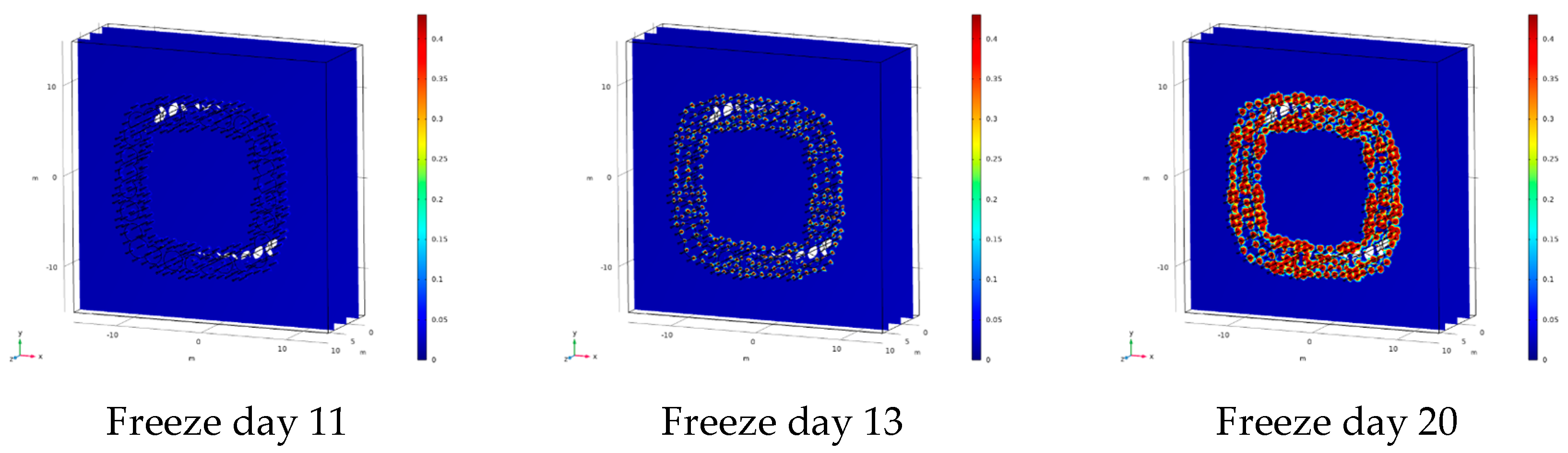
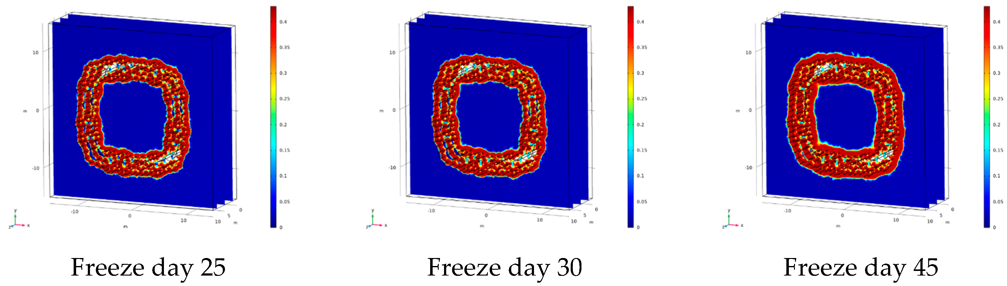
4.1. Temperature Field Calculation Results

In any freezing project, understanding the development of the temperature field is crucial for analyzing the freezing effect. Thus, the temperature field changes in the spatial section of freezing for 10, 20, 30, and 45 days were extracted, and freezing temperature iso-surface diagrams were constructed, as shown in Figure 4. As seen in Figure 4, to avoid the adverse effects of freezing caused by rapid heat exchange, the cooling pipe maintains the same temperature as the initial ground temperature at the beginning of cooling. On the first day of freezing, a single-hole temperature development mode is observed with the freezing pipes all reduced to below 18 °C. By the 10th day of freezing, the temperature of the freezing pipes reaches the critical phase change temperature of 0 °C. By the 20th day of freezing, the temperature of the freezing pipes reaches −18 °C, and that of the surrounding soil reduces to below the permafrost temperature of −1 °C, initiating the formation of the freezing curtain. Individual unconnected areas appear in the weak freezing zone. By the 30th day of freezing, the temperature of the freezing pipes reaches the lower limit of the freezing temperature at −28 °C. The soil in the weak freezing zone reaches temperatures below −20 °C, and the soil in the strong freezing zone reaches temperatures below −25 °C, resulting in the complete formation of the freezing curtain. By the 45th day of freezing, the freezing curtain significantly thickens, with the thickness of the frozen soil in the strong freezing zone significantly exceeding that in the weak freezing zone.

The length of the frozen pipe in this horizontal freezing project is the same, so the Z = 5 m section was analyzed to understand the characteristic changes over time. Specifically, the −1 °C and −10 °C isotherms for the Z = 5 m section were extracted after 15, 22, 25, 28, 30, and 45 days of freezing, as shown in Figure 5. Based on this figure, when the freezing pipe brine temperature reaches −10 °C on the 15th day of freezing, the −1 °C and −10 °C isotherms expand outward from the freezing pipe in concentric circles. In the weak freezing zone, the cold volume is more dispersed, causing the −1 °C isotherms to be scattered. Conversely, the −1 °C isotherms link more quickly in the strong freezing zone, indicating a faster intersection of the circles in the strong freezing zone. By the 22nd day of freezing, the −1 °C isotherms of both freezing zones’ outer and inner walls intersect. However, the contour has noticeable irregularities and an uneven temperature distribution. A clear temperature gradient exists between the strong and weak freezing zones. Additionally, due to the obstruction from the pipe curtain structure, the soil within the gaps of the pipe curtain cools more slowly, preventing the full formation of a permafrost structure. The strong freezing zone forms −10 °C permafrost associations, while the weak freezing zone shows a gradual expansion of −10 °C permafrost columns. By the 25th day of freezing, the inner and outer freezing walls of −1 °C and −10 °C intersect. By the 28th day, the outline of the curtain in both the strong and weak freezing zones becomes smoother, the temperature gradient difference between the two zones decreases, and a complete −1 °C permafrost structure is formed. On the 30th day of freezing, a stable and solid permafrost curtain structure is achieved with the thickness of the permafrost curtain in both the strong and weak freezing zones meeting the design standards. By the 45th day, the irregularities of the permafrost curtain nearly disappear, the transition area between the two freezing zones becomes smoother, and the curtain expands further outward.

The freezing temperature in the soil body is an important basis for judging whether the permafrost curtain is formed. The cooling curve in the region can provide important data for its permafrost curtain development and the law of freezing and expansion effect; 1~5 monitoring points are extracted from the strong freezing area above, 6~7 monitoring points are extracted from the weak freezing area in the corner, and 8~9 monitoring points are extracted from the weak freezing area on both sides, as shown in Figure 6.

The temperature change curve for each monitoring point throughout the freezing process is illustrated in Figure 7. As seen in Figure 7, points 1 and 3 in the strong freezing zone are less directly affected by the cold source than other monitoring points. Consequently, the heat exchange process at these points takes longer. However, the cooling rate at point 3 changes drastically on the 28th day of freezing. This phenomenon, when considered alongside the isothermal analysis, is attributed to the continuous development of the freezing front. During this period, a significant temperature gradient exists at both ends of point 3, prompting bidirectional heat transfer and an acceleration in the cooling rate. By the 35th day of freezing, point 1 reaches −10 °C, indicating that the inner edge of the stable frozen soil curtain formed by this freezing project has developed to point 1. Points 2, 4, and 5 in the strong freezing zone are directly affected by the cold source, resulting in a faster cooling process. The cooling rate slows significantly when the soil temperature reaches the phase transition temperature. This deceleration is due to the latent heat release required for the water in the soil to freeze, keeping the temperature near the freezing point during this stage. The soil temperature gradually decreases until most water completes the phase transition. This phenomenon is more pronounced closer to the cold source. After this phase, the cooling rate of the soil changes due to variations in parameters such as thermal conductivity. Additionally, compared to monitoring points 2 and 4, the cooling rate at point 5 is slower after the phase transition. This is mainly because point 5 is closer to the outer wall of the permafrost curtain, where heat exchange with the external ground temperature soil affects the cooling rate.

The cooling curves of the monitoring points in different paths of the weak freezing zone exhibit varying cooling rates. The cooling rate at point 6 is faster than that at point 8, and the cooling rate at point 7 is higher than at point 9. Furthermore, after cooling is completed, the temperature at monitoring points in the upper corner paths of the weak freezing zone is lower than at those in the lateral side paths. This difference is due to the more compact distribution of freezing tubes in the corner paths, which are more influenced by the cold source from the strong freezing zone.

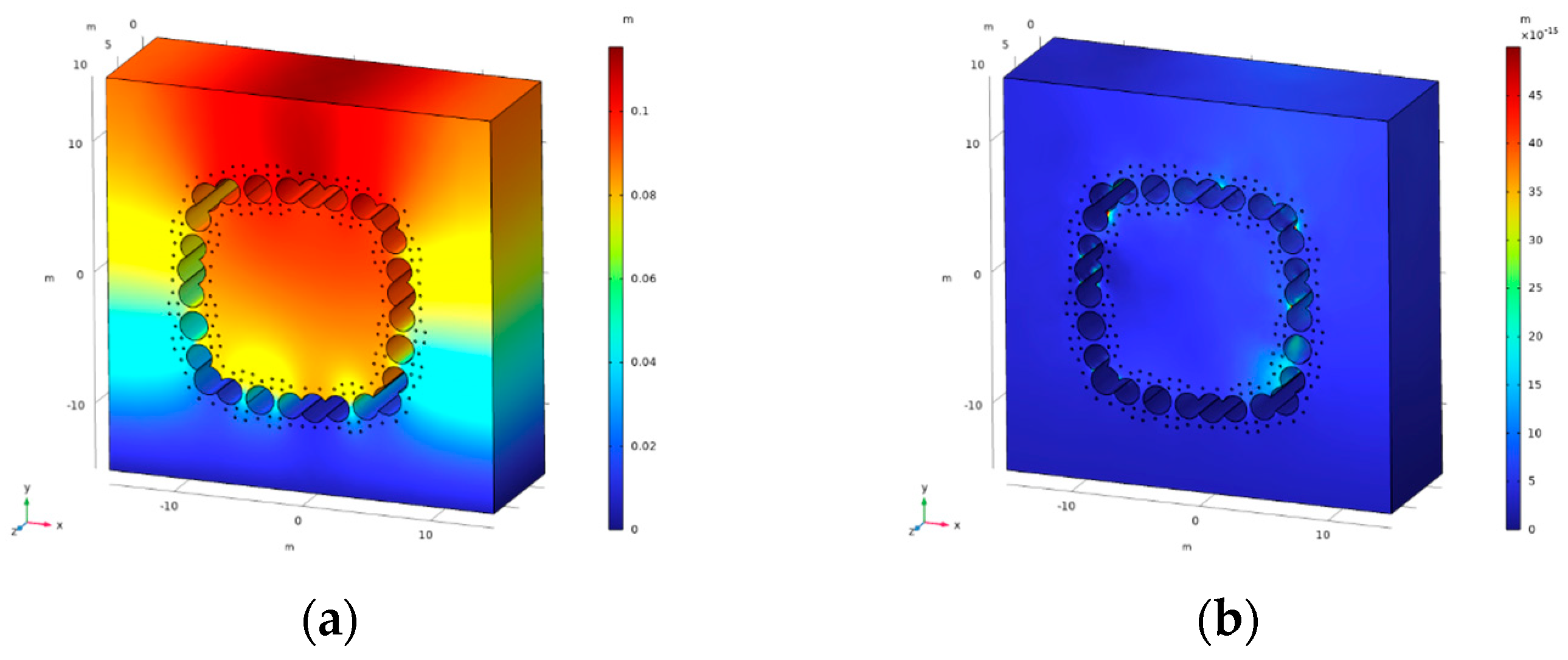
4.2. Moisture Field Calculation Results

In the freezing project, changes in the moisture field directly impact the effectiveness of the freezing process. Analyzing the changes in the moisture field can concretely reveal the moisture migration phenomena that occur during the formation of the freezing wall. Therefore, volume changes in ice content distribution were extracted at intervals of 11, 13, 20, 25, 30, and 45 days, as shown in Figure 8.

From this figure, it can be observed that by the 11th day of freezing, the temperature of the frozen tube had dropped below 0 °C, initiating fluctuations in the volumetric ice content centered around the frozen tube. By the 13th day of freezing, the temperature of the freezing tube continued to fall, causing the liquid water in the surrounding soil to condense into ice, although the ice content in the frozen soil column remained low at this stage. On the 20th day of freezing, the ice content in the soil of the strong freezing zone reached 35%, compared to the 40% volumetric water content before freezing. This indicated higher ice content–soil associations within the strong freezing zone. Conversely, the weak freezing zone only exhibited further expansion of the frozen soil column due to differences in the distribution of freezing tubes. By the 25th day of freezing, the surrounding soil had gradually formed a permafrost curtain rich in ice content. The ice content in the strong freezing zone was fuller and richer than in the weak freezing zone. Additionally, the volumetric ice content exceeded 40%, which is attributed to the approximately 9% volume expansion when water transitions to ice. On the 30th day of freezing, the ice content in the soil between the interconnecting steel pipes and the independent steel pipes within the pipe curtains increased significantly.

In contrast, the ice content at the edge of the freezing front was smaller than that near the frozen tube. This indicated that after freezing commenced, internal water migration occurred within the soil due to the temperature difference. The formation of a temperature gradient between the frozen and unfrozen areas led to the development of a moisture potential gradient. The moisture potential was lower in the freezing area and higher in the unfrozen area. Consequently, moisture migrated from the higher moisture potential in the unfrozen area to the lower in the freezing area, causing liquid moisture in the surrounding soil to spontaneously move toward the freezing front. This migration resulted in a higher unfrozen water content at the edge of the freezing front. By the 45th day of freezing, continuous moisture migration from the external and internal unfrozen soil and ongoing phase changes caused the freezing front to advance further. The thickness of the ice-bearing permafrost increased significantly, and the concavity of the inner and outer walls of the permafrost curtain became smoother, leading to a more uniform ice content distribution.

To further analyze the changing pattern of the moisture field, cloud plots of saturation changes were extracted for 20, 25, 30, and 45 days of freezing, as shown in Figure 9.

This figure shows that by the 20th day of freezing, the strong and weak freezing zones form a frozen soil structure. The weak freezing zone exhibits higher saturation around it due to differences in freezing efficiency. The soil saturation around the freezing pipe within the strong freezing zone is lower. The soil near the freezing pipe along the edge shows a temporary increase in saturation due to continuous moisture migration from the unfrozen soil to the cold zone, resulting in a decrease in soil saturation around the curtain. By the 25th day of freezing, a continuous freezing wall gradually forms around the freezing pipe. During this process, the outer edge of the curtain expands outward, and the inner edge expands inward. As external and internal moisture continues to gather in the cold zone, the internal moisture of the curtain essentially freezes, leading to significantly lower saturation. Overall, the soil saturation decreases with a smaller decrease observed further from the freezing pipe. Closer to the cold zone, the migration phenomenon becomes more pronounced. On the 30th day of freezing, the permafrost saturation distribution within the freezing curtain is uniform, approaching a very low value (near zero). In actual projects, saturation may not reach zero entirely because water in the soil exists in complex forms, such as adsorbed water and capillary water, which strongly interact with soil particles. Additionally, when water freezes into ice, it expands, causing the soil to expand and potentially altering the pore structure. Thus, even if the water freezes, the remaining pore space may not be empty, preventing the saturation from reaching zero. By the 45th day of freezing, the area of lower saturation further expands, enhancing the thickness of the frozen curtain. The ‘foggy’ appearance in the figure characterizes water migration. The inner edge of the frozen curtain appears smooth, with uniformly distributed soil saturation inside the curtain, indicating that water migration is nearing equilibrium. In contrast, the outer edge of the curtain has an obvious ‘tooth-like’ appearance, and the nearby soil shows a ‘foggy’ appearance, indicating intense water migration. The saturation at the outer edge of the curtain is higher than at the inner edge because the soil inside the curtain is a closed system with limited water migration and a small volume. In contrast, the soil outside the curtain is larger in volume, allowing for more significant water migration.

By analyzing the variation pattern of the volumetric water content of the soil, the range of locations susceptible to freezing can be obtained to intuitively reflect the freezing process of unfrozen water volume content changes. Considering the above analysis, seven representative typical paths were selected, namely 1~5 for the strong freezing zone monitoring points, 6~7 and 8~9 for the weak freezing zone monitoring points, 10~14 and 15~19 for the internal soil monitoring points, and 20~24 and 25~29 for the external soil monitoring points; each monitoring point was separated by a 1 m interval. Twenty-nine external soil monitoring points were used, and each monitoring point was separated by a 1 m interval, as shown in Figure 10.

The water content change curves for each monitoring point throughout the freezing process are illustrated in Figure 11. This figure shows that before the brine temperature of the freezing tube is reduced to the ice–water phase transition temperature, the water content at each monitoring point remains consistent with the original soil water content. When the brine temperature of the freezing tube reaches the phase transition temperature, the soil closer to the freezing tube experiences a rapid decline in water content, which tends to stabilize after a certain period of freezing. This phenomenon occurs because under the cooling effect of the freezing tube, the neighboring soil rapidly freezes, triggering a sharp soil moisture-to-pore ice phase change and causing a faster decrease in water content.

In the later stages of freezing and in conjunction with the previous analysis results of the temperature field, it is evident that the lower the freezing temperature, the smaller the water content at that location, as more moisture in the soil undergoes a phase change into ice. Monitoring point 3, which is farther from the freezing pipe, exhibits the lowest water content in the late freezing stage. This is attributed to its position in the gap of the pipe curtain structure, forming a closed area when the complete frozen soil curtain is established. The freezing wall prevents moisture migration from the unfrozen soil to this area, resulting in lower water content.

Additionally, the water content of the soil near the freezing pipe in the weak freezing zone at the corner decreases faster than in the weak vertical freezing zone. This is because the cooling rate at the corner location is faster, and the soil is more affected by the cold source. Overall, the change in water content can be divided into three stages. Firstly, the water content decreases slowly as the moisture in the soil migrates toward the freezing front with the distant moisture migration being less than the rate of moisture migration toward the freezing front. In the second stage, as the freezing front progresses toward this location, the moisture in the soil undergoes a phase change to pore ice, causing a rapid decrease in water content. Finally, when the temperature stabilizes, no more moisture undergoes a phase change, and the water content reaches a steady state. In soils outside the development of the freezing front, the water content decreases slowly. The decrease in water content is not significant due to distant moisture migration, and the further away from the freezing tube, the weaker the second-phase phenomenon becomes. Additionally, the water content of the soils inside the annular freezing curtain is lower than that of the area outside the curtain. In conjunction with the above analyses, this difference is due to the isolation of internal and external soil moisture migration processes by the annular freezing curtain.

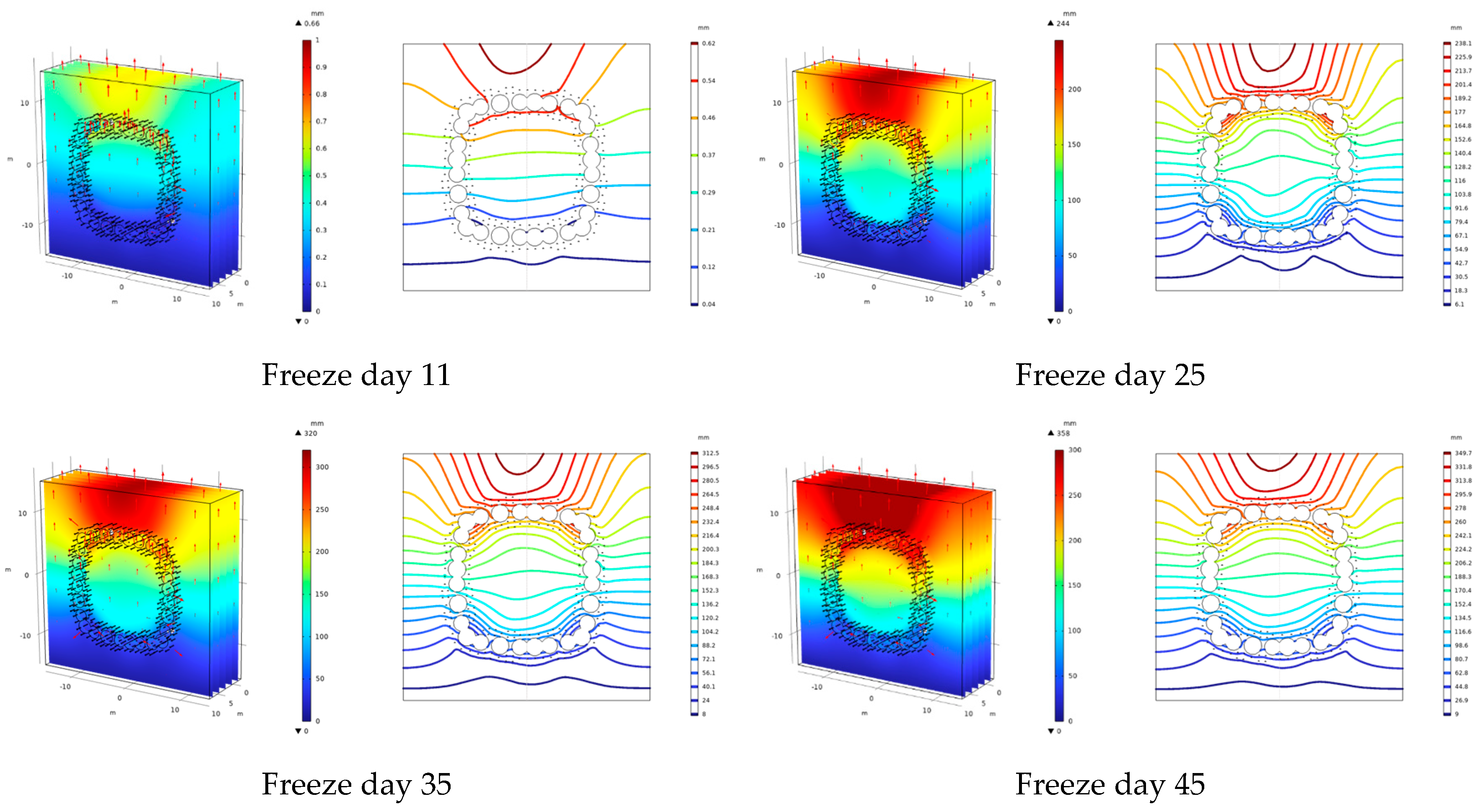
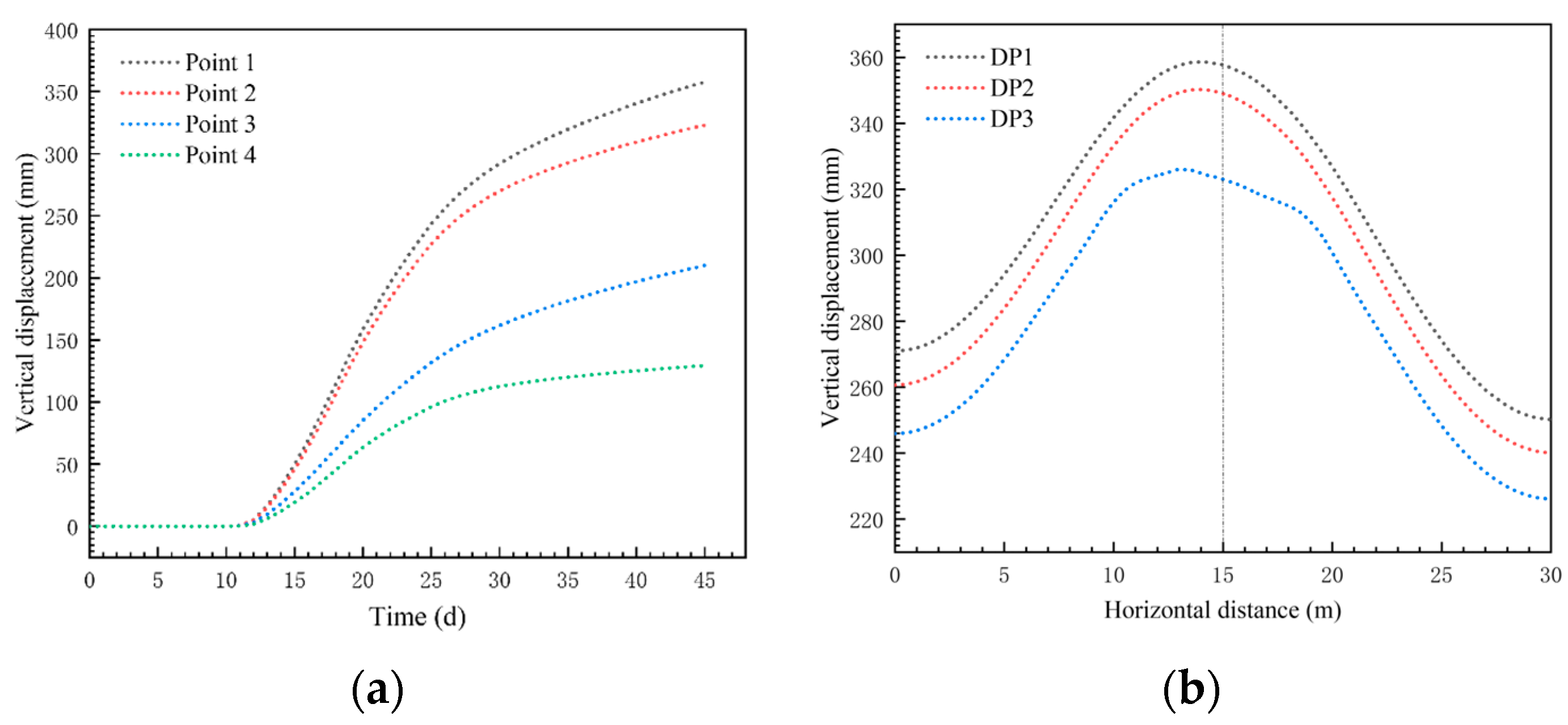
4.3. Displacement Field Calculation Results

Based on the above-mentioned research, the temperature evolution characteristics and moisture migration patterns during the freezing process have been revealed. However, the study of the project’s freezing law necessitates an analysis of soil freezing displacement, particularly vertical displacement. The magnitude of vertical displacement and ground surface uplift is a crucial index for assessing the stability and safety of the construction project and a prerequisite for the study of freezing displacement control, serving as an effective reference.

In calculating the ground deformation displacement field, the initial ground stress is generally caused by the self-gravity stress of the soil body. Given that the soil is typically consolidated before freezing, it can be assumed that its initial displacement is zero, and any subsequent displacement is mainly due to freezing expansion. If gravity is directly applied in the calculation, the software will automatically calculate a large initial displacement. Therefore, before calculating the displacement due to freezing and expansion effects, the initial displacement caused by gravity must be deducted to ensure the accuracy of the simulation results.

In this section, it is necessary to balance the ground stress through two steps before calculating the displacement due to freezing and expansion. First, the stress and displacement under gravity are calculated. The self-gravitational stress calculated in the first step is then extracted as the initial stress for the second study, and the displacement value from the first step is deducted. This ensures that the initial displacement in the calculation of freezing and expansion is nearly zero and that only the initial ground stress remains, as shown in Figure 12.

As shown in Figure 13, vertical displacement spatial cloud maps and vertical displacement contour maps (Z = 5) were extracted and analyzed for freezing times of 11, 25, 35, and 45 days.

According to Figure 13, the vertical freezing expansion area of the stratum increases gradually with the development of the freezing curtain. The soil near the frozen pipe concentration area in the upper part of the stratum exhibits larger vertical freezing displacement. This is primarily because the pipe curtain inhibits soil freezing displacement, but the overburden depth is shallow. Consequently, the freezing curtain volume and moisture accumulation area are larger. As freezing time progresses, the upward vertical displacement continually accumulates, leading to greater displacement at the top and surface location of the soil. In contrast, the bottom experiences smaller freezing displacement for two main reasons: the model’s boundary conditions limit the displacement, and the ground pipe curtain structure suppresses the freezing expansion at the bottom. Additionally, the effective stress of the soil body increases with depth, counteracting some of the freezing expansion forces generated during the freezing process.

The contour plot shows that at 11 days of freezing, the soil body only produces a small displacement due to the recent onset of the phase transition process. The freezing expansion occurs primarily near the freezing pipe, and the soil near the surface shows a vertical displacement of only 0.66 mm. By 25 days of freezing, the maximum vertical displacement of the soil near the surface reaches 244 mm. At 35 days of freezing, this maximum vertical displacement increases to 320 mm. During the 11-to-35-day interval, the phase change process is rapid, resulting in larger displacements. At 45 days of freezing, the development of the freezing curtain slows, the moisture accumulation area expands, and moisture migration continues. The maximum vertical displacement near the surface reaches 358 mm, indicating that the freezing displacement develops more slowly at this stage. The internal ice and water phase change gradually reaches an equilibrium state. In the region affected by the upward force of the pipe curtain structure, the contour interval is larger, indicating that the pipe curtain structure inhibits freezing and expansion displacement to some extent. The soil near the freezing pipe has dense contour lines, reflecting this region’s intense phase change process and the obvious freezing and expansion effect. The soil within the freezing curtain is directly subjected to minimal freezing effects with the displacement changes primarily being influenced by the lower freezing region and the effects of the curtains on both sides. Consequently, its displacement growth is slow, and the contour interval is larger.

To further analyze the vertical displacement pattern of the soil in the area near the surface during freezing, three monitoring paths, DP1 to DP3, and four monitoring points in the Z = 5 m section, point 1 to point 4, were selected, as shown in Figure 14.

The vertical displacement change for points 1 to 4 under different freezing times, as shown in Figure 15a, reveals that in the early-phase change phase, the surface area soil is influenced by all freezing pipes. The combined effect of freezing and the expansion of the underlying soil causes a significant uplift displacement in the surface area soil. Point 4, affected by the lower freezing zone, exhibits a displacement of 125 mm throughout the freezing process. There is no drastic increase in displacement between points 4 and 3 due to the minimal influence of the freezing pipes. The substantial displacement increase at the early freezing stage primarily occurs between points 3 and 2. No significant displacement difference is observed between points 1 and 2 because the freezing area has yet to develop to the top of point 2. However, the soil above point 2 experiences significant displacement with prolonged freezing time. As the freezing time continues, the freezing curtain develops further, and the moisture accumulation area expands, increasing displacement differences above the monitoring points. Once moisture migration reaches dynamic equilibrium, the displacement difference stabilizes, and the vertical displacement of the soil body below develops slowly.

From the vertical displacement observed after 45 days of freezing in Figure 15b, it is evident that larger vertical displacement differences primarily occur in areas directly affected by the cold source and the moisture accumulation area. Above DP2, no significant displacement changes are observed, which is mainly because the soil is already at the edge of the freezing curtain’s influence, where minimal phase change effects occur. Contour plots and path analysis diagrams indicate that the soil displacement is not symmetrically distributed along the center plane (X = 0), and the maximum displacement is not at the center point. This asymmetry is due to the denser distribution of freezing tubes on the left side, resulting in a greater freezing effect.

Finally, the analysis of vertical freezing displacement changes suggests that freezing causes significant surface uplift due to water migration. This phenomenon poses substantial engineering challenges, necessitating freezing control measures in the soil layers most adversely affected. Such measures are essential to prevent the deformation and rupture of pipelines in the upper ground and significant settlement during foundation thawing.

4.4. Sensitivity Analysis

According to previous research, the cooling plan is the most significant factor affecting the temperature change in freezing construction. Considering that the focus of the freezing project was on keeping the other material parameters of the soil body unchanged, we set the final brine temperatures to −23 °C and −33 °C and compared the results with those corresponding to the original −28 °C brine temperature to discuss the effect of the difference in the final temperature of the cooling plan on the temperature field and the displacement field. The cooling plan is shown in

Table 3. Salt water cooling program.

Time/d	0	20	30	45
Plan 1/°C	18	−20	−28	−28
Plan 2/°C	18	−25	−33	−33
Plan 3/°C	18	−15	−23	−23

.

Temperature variations measured in points 2 and 7 under different brine cooling plans were extracted and plotted, as shown in Figure 16 (certain details have been omitted for brevity). Analyzing the temperatures at the measurement points, it can be seen that due to the cooling plans all being the same at the beginning of freezing, differences between the cooling plans start to appear only after the cooling plans reach the lowest design plan, and the temperature differences are gradually shown after five days of active freezing: Plan 2 reaches the phase transition temperature faster and enters into the latent heat of the phase transition stage earlier than the original plan, while Plan 3 reaches the phase transition temperature slower and enters into the latent heat of phase transition stage at a time lag compared with the original plan. Afterward, as the minimum temperature of the brine cooling plan decreases, the temperature difference between the temperature measurement points gradually becomes larger. The overall law of cooling maintains the pre-freezing temperature decline speed; the soil body reaches the latent heat stage after slowing down and then starts to become faster before finally slowing down to a constant temperature, being lower than the design requirements of the permafrost temperature. The brine cooling program has a more obvious influence on the final freezing temperature. The temperature difference between the lowest temperature of the cooling program is 5 °C, and the final temperature difference between the temperature measurement points is about 5 °C.

The frozen vertical displacement variation curves of the DP1 path after freezing for 45 d under different brine cooling plans were extracted and plotted, as shown in Figure 17. As can be seen in this figure, the surface’s maximum vertical displacements of 379 and 213 mm were produced by 45-day freezing via Plans 2 and 3, respectively. The lower brine temperature has a wider range of influence, and the difference in displacement between the soils is farther away from the center of influence, while that of the center soil is smaller. In addition, the decrease in freezing displacement brought about by the increase in the minimum brine temperature is larger than the increase in displacement brought about by the decrease in the minimum brine temperature because when the minimum brine temperature increases, the thickness of its permafrost curtain decreases, and the phenomenon of soil freezing shrinkage is less obvious.

The above analysis implies that the cooling plan variation significantly influences the freezing law. Comprehensively considering the freezing effect reduction in the freezing process, the economic cost issue, and reinforcing effect, one can improve the minimum brine temperature according to a particular project’s conditions.

5. Conclusions

Based on the secondary development functions of the PDE module in COMSOL finite element software, this study performed three-field coupling simulations to preliminarily assess the freezing and expansion characteristics of a tunnel reinforcement process in Hainan, China. This study focused on analyzing the development of the freezing wall, changes in the moisture field, and vertical freezing and expansion displacement. The main conclusions that can be drawn from this study are as follows:

(1)

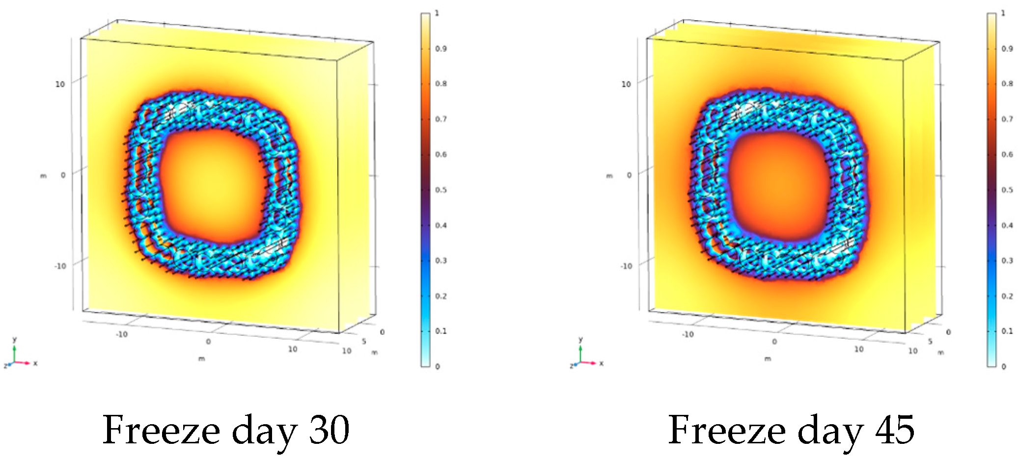
On the 25th day of freezing, temperature variation cycles from −1 to −10 °C were completed. By the 30th day, a fully frozen curtain had formed, meeting the design requirements for thickness. This indicates that the original cooling plan for the project was relatively conservative. Future optimizations could consider shortening the freezing period and reducing costs, referring to the temperature field analysis for improvements. The soil in the strong freezing zone exhibited a faster cooling rate and greater permafrost thickness than the weak freezing zone. The intervals between the pipe curtains in the strong freezing zone enhance the stability of the gaps and the water-stopping capability, aligning with the project’s requirements.

(2)

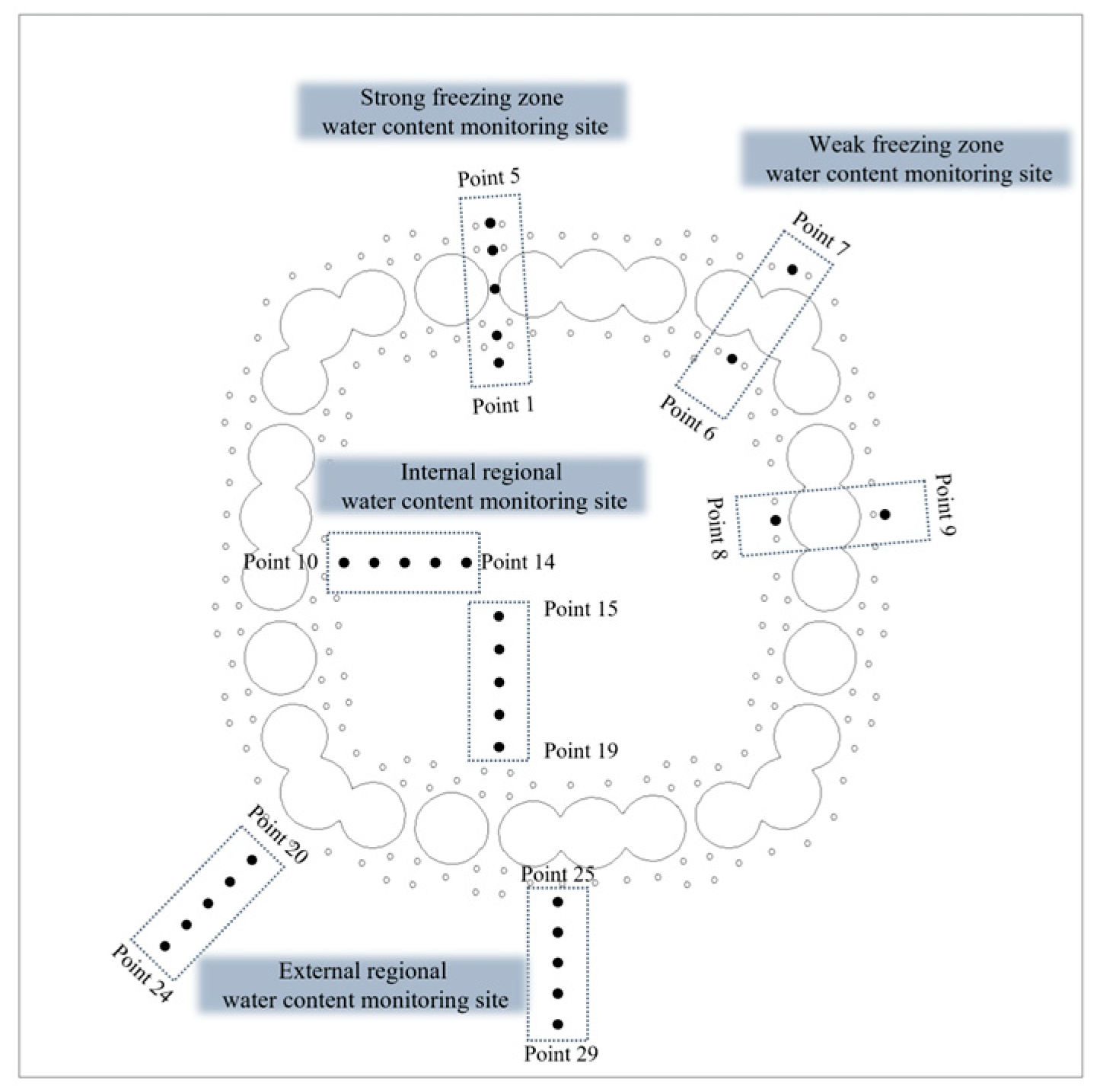
The influence of the freezing pipes on the soil area resulted in changes in the cooling rate at specific time nodes during the freezing process. Different monitoring points showed varying cooling rates due to differences in the influence of the cold source. Based on monitoring data, specific areas can be targeted for freezing control measures, allowing for adjustments to the freezing program in this project or similar ones.

(3)

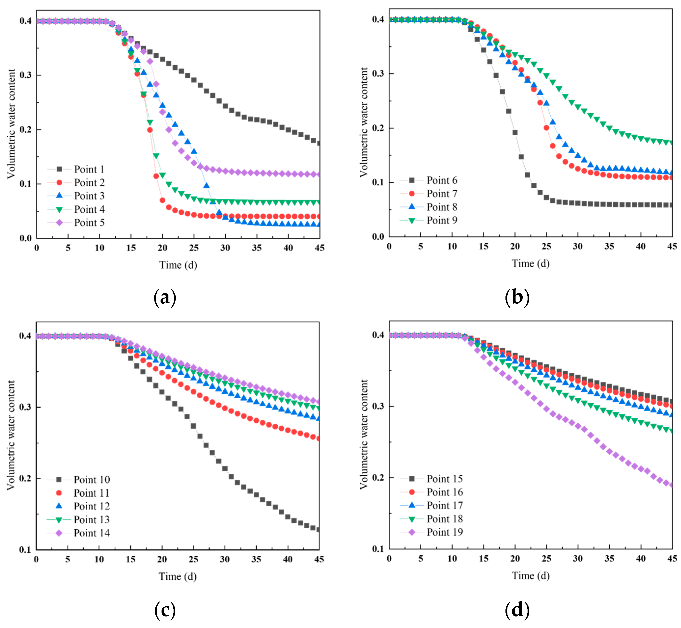
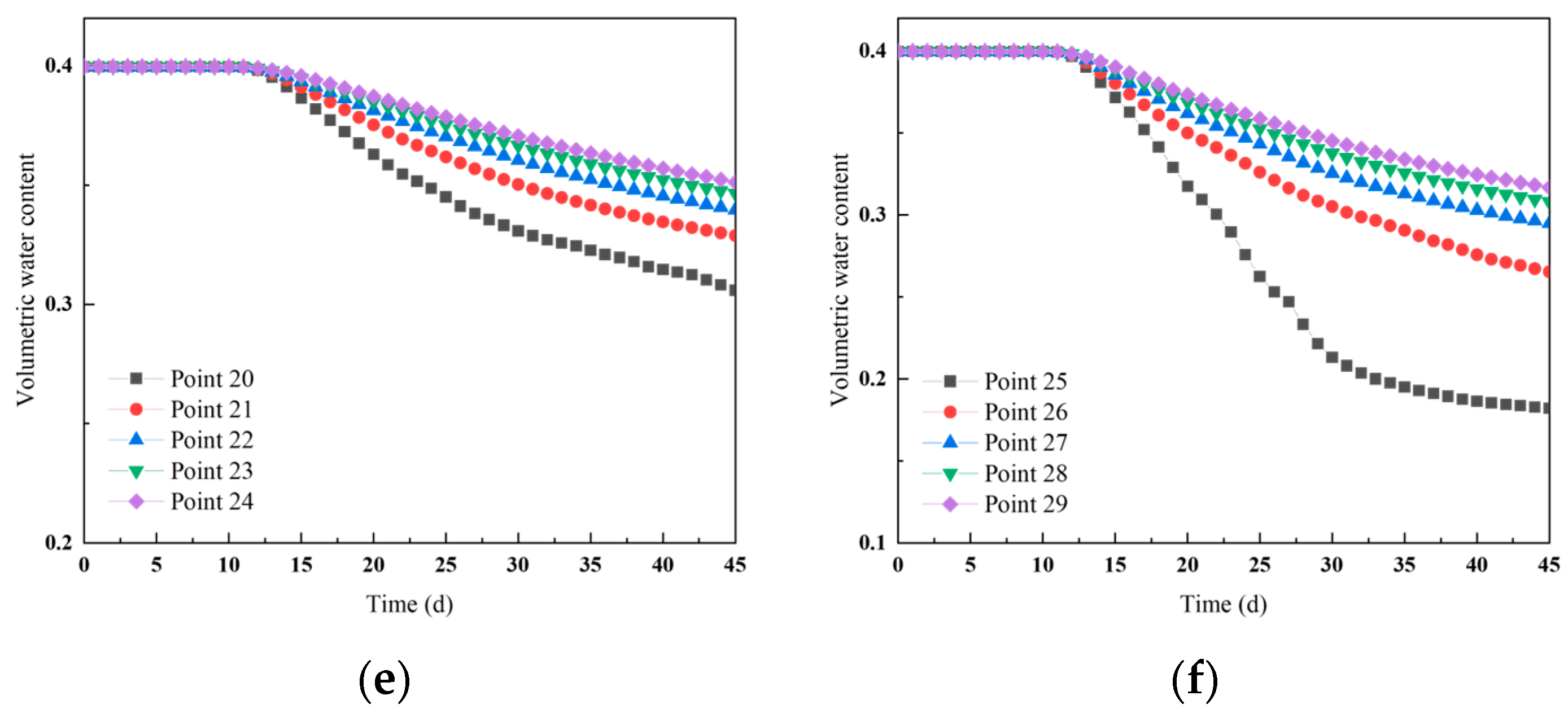
The ice content in the strong freezing area was higher than that in the weak freezing area. Due to the temperature gradient, moisture in the soil migrated toward the cold area, causing the saturation and water content of the surrounding soil to decline. Near the freezing pipe, moisture migration led to temporary water accumulation and increased saturation. By the 30th day of freezing, saturation within the curtain became uniform and approached zero with higher ice content marking the primary area of freezing and expansion effects. The saturation along the inner and outer edges of the curtain was slightly higher than inside the curtain due to moisture migration. Analyzing the saturation changes during freezing effectively elucidates the relationship between moisture migration and freeze-up.

(4)

The soil closer to the freezing pipe experienced a faster rate of water content reduction, eventually reaching a stable water content stage. The soil farther from the freezing pipe initially showed a slight decrease in water content. If later affected by the freezing front’s cold source, a change in the water content reduction rate can be observed; otherwise, only a slight decrease due to water migration occurs. Our analysis of moisture field changes suggests that regions with a rapidly increasing water content decrease, indicating significant moisture phase change to ice, corresponding to strong freezing effects.

(5)

In the early-phase change phase, frost heave was observed only near the freezing pipe, with the soil near the surface experiencing a vertical displacement of 0.66 mm. By the 35th day of freezing, upward freezing displacement continued accumulating after forming a stable freezing curtain with the maximum vertical displacement near the surface reaching 320 mm. On the 45th day, maximum freezing displacement reached 358 mm, indicating a decreased freezing heave effect in the later stages. Therefore, in actual projects, the focus should be on controlling the freezing effect before the 35th day. Additionally, dense contour lines near the freezing pipe indicated strong freezing displacement in that area, causing significant surface uplift. The maximum displacement was not centered in the construction soil but in the X-negative direction. The high water content in the powdery clay-based layer resulted in a pronounced frost expansion effect. The analysis in this paper provides a clear understanding of areas with significant frost expansion effects, offering a reference for assessing freezing programs and developing frost expansion control measures in this project or similar ones.

References

1. Alzoubi, M.A.; Xu, M.; Hassani, F.P.; Poncet, S.; Sasmito, A.P. Artificial ground freezing: A review of thermal and hydraulic aspects. Tunn. Undergr. Space Technol. 2020, 104, 103534. [Google Scholar] [CrossRef]
2. Hu, X.D.; Zhang, L.Y. Artificial ground freezing for rehabilitation of tunneling shield in subsea environment. Adv. Mater. Res. 2013, 734, 517–521. [Google Scholar] [CrossRef]
3. Zhou, J.; Li, Z.-Y.; Wan, P.; Tang, Y.-Q.; Zhao, W.-Q. Effects of seepage in clay-sand composite strata on artificial ground freezing and surrounding engineering environment. Chin. J. Geotech. Eng. 2021, 43, 471–480. [Google Scholar]
4. Hu, J.; Liu, Y.; Li, Y.; Yao, K. Artificial ground freezing in tunnelling through aquifer soil layers: A case study in Nanjing Metro Line 2. KSCE J. Civ. Eng. 2018, 22, 4136–4142. [Google Scholar] [CrossRef]
5. Huang, S.; Guo, Y.; Liu, Y.; Ke, L.; Liu, G. Study on the influence of water flow on temperature around freeze pipes and its distribution optimization during artificial ground freezing. Appl. Therm. Eng. 2018, 135, 435–445. [Google Scholar] [CrossRef]
6. Mauro, A.; Normino, G.; Cavuoto, F.; Marotta, P.; Massarotti, N. Modeling artificial ground freezing for construction of two tunnels of a metro station in Napoli (Italy). Energies 2020, 13, 1272. [Google Scholar] [CrossRef]
7. Ren, J.; Wang, Y.; Wang, T.; Hu, J.; Wei, K.; Guo, Y. Numerical Analysis of the Effect of Groundwater Seepage on the Active Freezing and Forced Thawing Temperature Fields of a New Tube–Screen Freezing Method. Sustainability 2023, 15, 9367. [Google Scholar] [CrossRef]
8. Zhang, C.; Yang, W.; Qi, J.; Zhang, T. Analytic computation on the forcible thawing temperature field formed by a single heat transfer pipe with unsteady outer surface temperature. J. Coal Sci. Eng. 2012, 18, 18–24. [Google Scholar] [CrossRef]
9. Zhou, X.; Jiang, G.; Li, F.; Gao, W.; Han, Y.; Wu, T.; Ma, W. Comprehensive review of artificial ground freezing applications to urban tunnel and underground space engineering in China in the last 20 years. J. Cold Reg. Eng. 2022, 36, 04022002. [Google Scholar] [CrossRef]
10. Hu, J.; Li, K.; Wu, Y.; Zeng, D.; Wang, Z. Optimization of the Cooling Scheme of Artificial Ground Freezing Based on Finite Element Analysis: A Case Study. Appl. Sci. 2022, 12, 8618. [Google Scholar] [CrossRef]
11. Alzoubi, M.A.; Sasmito, A.P.; Madiseh, A.; Hassani, F.P. Intermittent freezing concept for energy saving in artificial ground freezing systems. Energy Procedia 2017, 142, 3920–3925. [Google Scholar] [CrossRef]
12. Alzoubi, M.A.; Sasmito, A.P.; Madiseh, A.; Hassani, F.P. Freezing on demand (FoD): An energy saving technique for artificial ground freezing. Energy Procedia 2019, 158, 4992–4997. [Google Scholar] [CrossRef]
13. Tounsi, H.; Rouabhi, A.; Jahangir, E. Thermo-hydro-mechanical modeling of artificial ground freezing taking into account the salinity of the saturating fluid. Comput. Geotech. 2020, 119, 103382. [Google Scholar] [CrossRef]
14. Tounsi, H.; Rouabhi, A.; Tijani, M.; Guérin, F. Thermo-hydro-mechanical modeling of artificial ground freezing: Application in mining engineering. Rock Mech. Rock Eng. 2019, 52, 3889–3907. [Google Scholar] [CrossRef]
15. Auld, F.A.; Belton, J.; Allenby, D. Application of Artificial Ground Freezing. 2015. Available online: https://www.icevirtuallibrary.com/doi/abs/10.1680/ecsmge.60678.vol3.121 (accessed on 31 July 2024).
16. Joudieh, Z.; Cuisinier, O.; Abdallah, A.; Masrouri, F. Artificial Ground Freezing—On the Soil Deformations during Freeze–Thaw Cycles. Geotechnics 2024, 4, 718–741. [Google Scholar] [CrossRef]
17. Moriuchi, K.; Ueda, Y.; Ohrai, T. Study on the ad freeze between frozen soil and steel pipes for cutoff of water. Doboku Gakkai Ronbunshuu C 2008, 64, 294–306. [Google Scholar] [CrossRef]
18. Cheng, Y.; Ma, B.; Liu, J. Scheme designing of gongbei tunnel. Highw. Tunn. 2012, 3, 34–38. [Google Scholar]
19. Hu, X.; Fang, T. Numerical simulation of temperature field at the active freeze period in tunnel construction using freeze-sealing pipe roof method. Tunneling and underground construction. In Proceedings of the Geo-Shanghai 2014, Shanghai, China, 26–28 May 2014; pp. 731–741. [Google Scholar]
20. Hu, X.; Wu, Y.; Li, X. A field study on the freezing characteristics of freeze-sealing pipe roof used in ultra-shallow buried tunnel. Appl. Sci. 2019, 9, 1532. [Google Scholar] [CrossRef]
21. Hong, Z.; Hu, X.; Fang, T. Analytical solution to steady-state temperature field of Freeze-Sealing Pipe Roof applied to Gongbei tunnel considering operation of limiting tubes. Tunn. Undergr. Space Technol. 2020, 105, 103571. [Google Scholar] [CrossRef]
22. Niu, Y.; Hong, Z.Q.; Zhang, J.; Han, L. Frozen curtain characteristics during excavation of submerged shallow tunnel using Freeze-Sealing Pipe-Roof method. Res. Cold Arid Reg. 2022, 14, 267–273. [Google Scholar] [CrossRef]
23. Hong, Z.; Zhang, J.; Han, L.; Wu, Y. Numerical Study on Water Sealing Effect of Freeze-Sealing Pipe-Roof Method Applied in Underwater Shallow-Buried Tunnel. Front. Phys. 2022, 9, 794374. [Google Scholar] [CrossRef]
24. Duan, Y.; Rong, C.; Long, W. Numerical Simulation Study on Frost Heave during the Freezing Phase of Shallow-Buried and Undercut Tunnel Using the Freeze-Sealing Pipe Roof Method. Appl. Sci. 2023, 13, 10344. [Google Scholar] [CrossRef]
25. Cui, Z.D.; Zhang, L.J.; Xu, C. Numerical simulation of freezing temperature field and frost heave deformation for deep foundation pit by AGF. Cold Reg. Sci. Technol. 2023, 213, 103908. [Google Scholar] [CrossRef]
26. Russo, G.; Corbo, A.; Cavuoto, F.; Autuori, S. Artificial ground freezing to excavate a tunnel in sandy soil. Meas. Back Anal. Tunn. Undergr. Space Technol. 2015, 50, 226–238. [Google Scholar] [CrossRef]
27. Li, M.; Cai, H.; Liu, Z.; Pang, C.; Hong, R. Research on Frost Heaving Distribution of Seepage Stratum in Tunnel Construction Using Horizontal Freezing Technique. Appl. Sci. 2022, 12, 11696. [Google Scholar] [CrossRef]
28. Nishimura, S.; Gens, A.; Olivella, S.; Jardine, R.J. THM-coupled finite element analysis of frozen soil: Formulation and application. Géotechnique 2009, 59, 159–171. [Google Scholar] [CrossRef]
29. Taylor, G.S.; Luthin, J.N. A model for coupled heat and moisture transfer during soil freezing. Can. Geotech. J. 1978, 15, 548–555. [Google Scholar] [CrossRef]
30. Bai, Q.; Li, X.; Tian, Y.-H.; Fang, J. Equations and numerical simulation for coupled water and heat transfer in frozen soil. Chin. J. Geotech. Eng. 2015, 37, 131–136. [Google Scholar]
31. Tan, X.; Chen, W.; Tian, H.; Cao, J. Water flow and heat transport including ice/water phase change in porous media: Numerical simulation and application. Cold Reg. Sci. Technol. 2011, 68, 74–84. [Google Scholar] [CrossRef]
32. Tang, L.; Yang, L.; Wang, X.; Yang, G.; Ren, X.; Li, Z.; Li, G. Numerical analysis of frost heave and thawing settlement of the pile–soil system in degraded permafrost region. Environ. Earth Sci. 2021, 80, 1–19. [Google Scholar] [CrossRef]
33. Wang, L.; Zhou, J.; Qi, J.; Sun, L.; Yang, K.; Tian, L.; Lin, Y.; Liu, W.; Shrestha, M.; Xue, Y.; et al. Development of a land surface model with coupled snow and frozen soil physics. Water Resour. Res. 2017, 53, 5085–5103. [Google Scholar] [CrossRef]
34. Wu, J.; Han, T. Numerical research on the coupled process of the moisture-heat-stress fields in saturated soil during freezing. Eng. Mech. 2009, 26, 246–251. [Google Scholar]
35. Fu, Y.; Hu, J.; Wu, Y. Finite element study on temperature field of subway connection aisle construction via artificial ground freezing method. Cold Reg. Sci. Technol. 2021, 189, 103327. [Google Scholar] [CrossRef]
36. Hu, J.; Yang, P.; Dong, Z.; Cai, R. Study on numerical simulation of cup-shaped horizontal freezing reinforcement project near shield launching. In Proceedings of the 2011 International Conference on Electric Technology and Civil Engineering (ICETCE), Lushan, China, 22–24 April 2011; IEEE: Piscataway, NJ, USA, 2011; pp. 5522–5525. [Google Scholar]
Figure 1. Schematic diagram of freezing pipe arrangement.
Applsci 14 07106 g001
Figure 2. Physical field coupling relationship diagram.
Applsci 14 07106 g002
Figure 3. Schematic diagram of the geometric mode (a) and meshing (b).
Applsci 14 07106 g003
Figure 4. Temperature cloud maps and equivalence surface maps at different freezing times.
Applsci 14 07106 g004
Figure 5. Isotherm plots of −1 °C and −10 °C for cross-sections at different freezing times.
Applsci 14 07106 g005
Figure 6. Schematic of cross-section temperature monitoring points.
Applsci 14 07106 g006
Figure 7. (a) Temperature changes at monitoring points 1 to 5 in the strong freezing zone; (b) temperature change at monitoring points 6~7 in the weak freezing zone; and (c) temperature change at monitoring points 8~9 in the weak freezing zone.
Applsci 14 07106 g007
Figure 8. Volumetric ice content cloud maps at different freezing times.
Applsci 14 07106 g008aApplsci 14 07106 g008b
Figure 9. Cloud maps of soil saturation change.
Applsci 14 07106 g009aApplsci 14 07106 g009b
Figure 10. Schematic of cross-section water content monitoring points.
Applsci 14 07106 g010
Figure 11. (a) Water content changes at monitoring points 1 to 5; (b) water content changes at monitoring points 6~9; (c) water content changes at monitoring points 10~14; (d) water content changes at monitoring points 15~19; (e) water content changes at monitoring points 20~24; and (f) water content changes at monitoring points 25~29.
Applsci 14 07106 g011aApplsci 14 07106 g011b
Figure 12. (a) Initial stress displacement; (b) displacement after geostress equilibrium.
Applsci 14 07106 g012
Figure 13. Cloud maps and contour maps of vertical displacement at different freezing times.
Applsci 14 07106 g013
Figure 14. Schematic diagram of freeze-up displacement monitoring path and monitoring points.
Applsci 14 07106 g014
Figure 15. (a) Variation in freezing vertical displacement of monitoring points under different times; (b) frozen vertical displacement map of each path after 45 d of freezing.
Applsci 14 07106 g015
Figure 16. (a) Comparison of temperature changes at point 2 under different freeze plans; (b) comparison of temperature changes at point 7 under different freeze plans.
Applsci 14 07106 g016
Figure 17. Comparison of surface frozen vertical displacement under different freeze plans for 45 d of freezing.
Applsci 14 07106 g017