Featured Application
A hybrid forecasting model with two subcomponents is presented in this study. A basic and secondary models are combined in a hierarchy to improve forecasting performance. This is particularly important for complex data sets with multiple patterns. Such data sets do not respond well to simple models, and hybrid models based on the integration of various forecasting tools often lead to better forecasting performance.
Abstract
This study involves the development of a hybrid forecasting framework that integrates two different models in a framework to improve prediction capability. Although the concept of hybridization is not a new issue in forecasting, our approach presents a new structure that combines two standard simple forecasting models uniquely for superior performance. Hybridization is significant for complex data sets with multiple patterns. Such data sets do not respond well to simple models, and hybrid models based on the integration of various forecasting tools often lead to better forecasting performance. The proposed architecture includes serially connected ARIMA and ANN models. The original data set is first processed by ARIMA. The error (i.e., residuals) of the ARIMA is sent to the ANN for secondary processing. Between these two models, there is a classification mechanism where the raw output of the ARIMA is categorized into three groups before it is sent to the secondary model. The algorithm is tested on well-known forecasting cases from the literature. The proposed model performs better than existing methods in most cases.
1. Introduction
A time series is a set of records collected over time. To be called a time series, the data should be ordered chronologically, with equal distance between observation points. A weekly sale of a particular item in a store would comprise a time series. Depending on circumstances, data may be collected hourly, daily, weekly, monthly, etc. Time-indexed data could be the subject matter of a diverse spectrum of research areas, including science, engineering, and finance. Such broad interest from different fields has led to the development of an assorted set of forecasting approaches.
Developing forecast models for time series can be challenging from several perspectives. In many instances, there is no insight into the underlying mechanism that generates data, hindering the development of a valid mathematical model. Empirical data are a product of a complex real-world mechanism (e.g., daily change in stock prices); standard statistical procedures may be inadequate to reveal the underlying relationships.
That built-up complexity in the data may exhibit itself as noise or be observed as nonstationary or nonlinear behavior. Noise is a natural phenomenon because many undetected variables impact the controlled variable. For effective modeling, the noise has to be appropriately identified and excluded by the model. Nonstationarity refers to the dynamic nature of the data. The underlying process that generates the data changes over time, and the model has to be capable of determining these changes. In the long run, almost all data series become nonstationary because of the dynamic nature of the underlying processes. This brings up the issue of determining the length of usable history, which is a challenging task. To further aggravate the issue, the noise in the series may vary with time. Nonlinearity is also another interesting issue. Most of the time, models are based on the assumption that the underlying relationship is linear, which may not be valid for all instances. There are many examples where it has been shown that the nonlinear model serves as a better fit for the data [1].
Inherent difficulties in time series modeling led researchers to look for creative alternatives. One popular method is to combine different forecasting models in a framework to enhance forecasting capability. This process is better known as hybridization, based on the following premise. Each modeling methodology has its superior aspects but may be weak in others, and it is possible to combine them in a framework to maximize the overall benefit.
Efforts to combine multiple forecasting models can be traced back to the pioneering work of Bates and Granger [2], in which two separate forecasts generated by different approaches are combined into one to minimize the variance. Many researchers followed the path opened by Bates and Granger [2] to develop creative hybrid models. With more accurate and reliable forecasts, hybrid models ranked top in prominent forecasting competitions. In a recent M4 competition, where each entrant had to generate forecasts for thousands of data sets, a hybrid model that combined exponential smoothing and recurrent neural networks came first by a solid margin [3]. The organizer of the M-competition, Prof. Makridakis, has the following comment about the hybrid models, which highlights the performance of hybrid models. “The accuracy when various methods are being combined outperforms, on average, the individual methods being combined and does very well in comparison to other methods” [4]. Our research contributes to this field with its unique structure of combining two standard forecasting methods.
The rest of the paper is organized as follows. In Section 2, we present a literature review focusing on previous work directly related to our research. In Section 3, we present methodology, including a brief mention of ARIMA models and ANN. Our approach and modeling details are given in this section. In Section 4, the performance of our model with respect to benchmarks is presented in detail. The concluding remarks, including future work, are given in Section 5.
2. Literature Review
Because of the broad nature of time series forecasting, the literature review is confined to previous works related directly to our proposed approach. The subject of hybridization, which covers umbrella structures combining different forecasting methods, can be divided into two broad categories. In the first category, each model runs independently and generates a separate forecast. These forecasts are then consolidated into a final number. The pioneering work of Bates and Granger [2] falls into this category. Their method involves generating two separate forecasts and then averaging them into a single number. In the second category, models are connected in series. Figure 1 shows a simple, serially connected model, where the output of the first model is directly fed into the second one. In this serial combination, the underlying implicit assumption is that the series can be decomposed into distinct sub-categories. Once the series is decomposed, we can handle each sub-category with a different model.
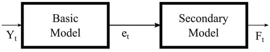
Figure 1.
A serially connected hybrid model.
For the serial combination of models, the earliest arrangement is proposed by Zhang [5], where ARIMA (autoregressive integrated moving average) and ANN are connected in series as basic and secondary models. Following this work, various serially connected models utilizing both linear and nonlinear methods have been proposed. Additionally, the original approach was fine-tuned for better performance [6].
The accumulated work on serially connected hybrid models can be further divided into two broad categories. The first category includes studies that propose a new forecasting method for basic or secondary models. The “new” methodology does not necessarily refer to an original approach, but it is something new within the context of serial hybridization. Here, the emphasis is on the novelty of the method used, and model verification and validation are often done by using popular data sets from the literature. The second category of research is about applications of hybrid models. This work aims to generate the most accurate forecast and often involves trial and error with multiple hybrid alternatives.
One caveat is that the categorization schema presented above is not clear-cut, and some works can claim novelty in terms of both methodology and the data sets involved. Within the framework of this broad division, the list of recent works for each category is listed below. For methodology-oriented research: autoregressive moving average (MARMA) and exogenous multi-variable input [7], ARIMAX (ARIMA with explanatory variables), Holt–winters, ANN [8], SARIMAX (seasonal ARIMA with explanatory variables), LSSVM (least-squares support-vector machine) [9], ARMAX, ANN [10], ARIMA and ANN [11,12,13], ARIMA and GNN (granular neural networks) [14]. For application-oriented research: wind speed forecasting [8,15], oil prices [12], tourist arrivals [16], monthly rainfall [9], computer network traffic [17], dengue epidemics [12], electricity consumption [18], power plant fuel consumption [19], stock market [20], and urban water demand [21].
Two interesting serial-model studies deserve special mention, as they are directly related to our work. In both studies, the output of the first model is not sent directly to the secondary model. Instead, the residuals, the difference between actual and fitted values, are analyzed and then sent to the second model according to a preset algorithm. The first approach proposed by Khashei et al. [6] combines ARIMA with PNN (probabilistic neural networks) as the first and secondary models. The PNN utilizes the error output of the ARIMA. Error values coming out of ARIMA are categorized, and each category is treated differently by PNN. The second study, by Babu and Reddy [22], also uses the ARIMA and ANN combination, and it has a similar error classification mechanism between the first and second models. The error output of the first model is classified according to the spread around the mean. For this purpose, the mean value for the error output of the first model and the accompanying deviation for each observation are calculated. Based on the magnitude of the deviation, observations are categorized as high- and low-volatility groups, and each group is treated differently by the ANN model.
3. Methodology
The proposed hybrid model has two components that are connected sequentially. The first one is called the basic model and includes ARIMA forecasting to capture the linear relationship of the input data. The output of the ARIMA is fed into the second component. A neural network model capable of capturing both linear and nonlinear patterns is used in the second component. As most data sets are composed of linear and nonlinear elements, two separate models that work in tandem will be more effective in capturing different portions of the data. Before moving into details of the hybrid model, brief descriptions of ARIMA, and ANN models are given below.
3.1. ARIMA Models
ARIMA is a popular forecasting tool used in time series forecasting. In this approach, the forecast is based on a linear combination of past values and random errors. The general formula for an ARIMA (p,d,q) model is given in Equation (1). Two primary components of ARIMA are autoregressive (AR) and moving average (MA) functions. The p and q parameters in Equation (1) represent the order of AR and MA functions, respectively. The third parameter, d, gives the number of differencings performed on the series to make it stationary.
where and represent the actual value and the error (offset between the actual and the fitted value). Parameter sets (i = 1, 2, …, p) and (j = 0, 1, 2, …, q) represent AR and MA sections of the ARIMA. The term (1 − B)d serves as a difference operator.
3.2. Artificial Neural Networks (ANNs)
ANNs are computational systems based on the operational structure of a biological brain. ANN architecture consists of units (i.e., neurons) that are organized in layers. In addition to the input and output layers, there are hidden layers between the input and the output. ANN is a nonparametric approach that can extract nonlinear dynamics from the data. Because of the limitations of statistical tools, ANN has long been regarded as an alternative route to deal with nonlinear problems in various fields. There are various architectures used in ANN, some of which mimic the function of the brain, but others are mathematical representations constructed according to the problem requirements. Among these varieties, MLP (multi-layer perceptron) has long been used for nonlinear regression problems.
A three-layer feed-forward neural network is commonly used in time series modeling (Figure 2). The input layer includes p nodes, each representing an input to the model ( through ). The middle (i.e., hidden) layer includes q units, and there is a single output . Each unit in the hidden layer processes the information fed from the input units. Links between the input and hidden layers are model parameters. Each link between the input and hidden layer has a weight . Similarly, the represents the weight of the link between the hidden and output layers.
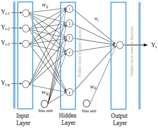
Figure 2.
Proposed neural network structure () [6].
3.3. Forecast Accuracy Metrics
The accuracy of a forecast can be assessed in several different ways. In this study, three standard metrics, MAD, MSE, and MAPE, are used to compare the performance of different forecasting methods. The MAD and MSE are scale-dependent metrics, and the magnitude of the error varies with the magnitude of the underlying series. On the other hand, the MAPE is a relative-error metric ranging between 0 and 1. The scale-independent nature of MAPE makes it a convenient assessment tool in a one-to-one comparison of time series with varying magnitudes. The formulation for each error metric is given in Equations (2)–(4).
- Mean Absolute Deviation (MAD)
- Mean Squared Error (MSE)
- Mean Absolute Percent Error (MAPE):where and represent the actual and the forecast. As we propose a new forecasting approach in this study, our primary focus is to compare the performance of the proposed method with respect to previous work. For a one-to-one comparison of different models, each model has to be tested on the same data set. In test runs, we used MAD and MSE to evaluate forecast accuracy. These two metrics are easy to compute and understand [23,24].
3.4. Hybrid Model
The proposed hybrid arrangement combines ARIMA and ANN models in series. As given in Equation (5), the original time series is considered the sum of two components: one is linear and the other is nonlinear. The linear component is represented by a multi-period lagged ARIMA model (Mt). This component captures the linear relationship in the data. The second component (Nt) is built on the leftover error of the first model. Whatever cannot be explained by ARIMA is fed into the ANN.
Based on the assumption that, the data can be split into two components, representing linear () and nonlinear () portions, a hybrid forecasting approach is developed to exploit the unique characteristics of each component. Processes involved in hybrid modeling can be divided into six sub-tasks performed in sequential order: (1) The routine starts with the basic model; (2) the error output of the basic model is processed in the classification; (3) based on the classification, the input lists are prepared for the second model; (4) the secondary model runs on each list separately; (5) the output of the second model is consolidated in hybridization; (6) in the final stage, projections are generated with the hybrid model. Figure 3 shows tasks and relationships graphically.
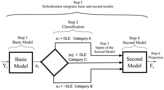
Figure 3.
Proposed hybrid structure.
- Step 1. The Basic Model
The modeling process starts with the division of the original time series into training and test series. Next, the basic model is developed using only the training data, which includes the first portion of the data set (i.e., the chronologically older). In terms of size, the training data are typically several times larger than the test portion. In selecting the split point, we followed the guidelines used in previous studies on the same data sets. It should be noted that the number of observations in the training data is further reduced because of the lag effect in the data. The formula for the basic model is given in Equation (6).
where and represent the actual and forecast values at point t. The offset between the two is the error , and it is used as a basis to construct a new time series for the second component.
- Step 2. Classification
In the second stage, the error output of the first component (Equation (7)) is classified into three distinct groups. The classification is done according to an a priori selected threshold value. Over-shooters include non-negative errors that are greater than the threshold. Under-shooters are negative errors that are smaller than the negative value of the threshold limit. Anything that falls between these two limits is categorized as neutral. This type of categorization was first proposed by Khashei et al. [25], where the threshold limits are defined as the desired level of error (DLE). The value of this parameter could be set by the user based on the analysis of the error coming from the basic model. In particular, the distribution of error coming from the basic model can provide insight regarding when or how the basic model over- or under-estimates. If there is no insight into the performance of the basic model, it could be set to a fixed value. For example, the DLE is set to 5% in experimental runs by Khashei et al. [25]. The error output of the basic model is categorized into three groups: A, B, and C, with the following definitions:
- , Category A
- , Category B
- , Category C
- Step 3. Input Lists for the Second Model
Based on the categorization of the second step, three separate data lists are constructed from the original error output in Equation (7). To explain the process, let us assume that the output of the basic model is stored in a list, E, with n members, . Three separate lists, A, B, and C, are generated from list E. While lists A and B represent underestimated and overestimated values of E, list C holds neutral error values. The content of E is directly copied to A, B, and C to initialize the lists. Then, with the guidelines given in Equation (8), adjustments are made to each list. In list A, which represents underestimated values, all category A values are kept as they are, but everything else is set to zero. Similarly, list B, representing overestimated errors (i.e., category B), retains its original values but overwrites everything else with zero. For list C, all elements with over- and underestimated values are set to zero.
- Step 4. The Second Model
The second model performs a complementary function. It uses leftover error values from the basic model to extract additional explanatory information. As explained in the previous step, the error output is categorized into three separate lists. The lists A and B represent under- and overestimated values, and they are the inputs for the second model. List C contains error values that remain below the threshold (i.e., DLE) and are excluded from the run. The second model includes an artificial neural network (ANN) to identify nonlinear patterns and any high-order linear relationships that the basic model missed. In the original approach proposed by Zhang [26], the primary and secondary models are assigned specific tasks. While the primary model deals with the linear component of the data, the leftover error is assumed to be the nonlinear component. This type of classification of the domain may not be applicable in every situation, and the residual error of the primary model cannot be presupposed as a nonlinear component. It is likely that the leftover error values are a combination of linear and nonlinear error values.
The ANN model is run separately on A and B lists to generate two sets of forecasts, representing the under- and overestimation portions of the model. As stated in Equations (9) and (10), the ANN uses n period-lagged values from t to t − n to generate the forecast for t + 1.
where and represent functions used by ANN. The terms and are random errors.
- Step 5. Hybridization
Hybridization involves integrating basic and secondary models in a schema to produce a single (i.e., hybrid) forecast. In the proposed schema, the hybrid forecast for t + 1 is the sum of outputs generated by and .
Forecasts given in (11) and (12) can be considered a modified version of the basic model forecast. The in (11) is the corrected version when the basic model underestimates the true value. Underestimation produces positive errors in the basic model. When positive values are fed into the secondary model, the secondary model, in turn, is likely to produce positive-valued forecasts. This could be considered compensation for the underestimation of the basic model. A reverse mechanism works in (12). When the basic model overestimates, errors are likely to be negative. To compensate, the second model will produce negative-valued forecasts ().
In addition to these two forecasts, the basic model’s direct output can be considered a third forecast. The second model is bypassed, and the output of the basic model is the final forecast: . The can be considered category C, and it represents the mid-value of three forecasts. While category C determines the midpoint, forecasts for A and B are upper and lower estimates. Among three candidate forecast points (i.e., ), one must be selected as the final forecast. The selection is based on the error metrics discussed in Section 3.3. The combination with the lowest score is chosen as the final hybrid model.
- Step 6. Projection
The hybrid model selected in the previous step is used for projection. Model selection is based on the performance of the training data, which are exclusively used for model development. Once the model is finalized, its forecasting performance is evaluated on the test data. This data set is a continuation of the training data and is used for model validation only.
In terms of platform and software, we used IBM’s SPSS statistical software to build ARIMA models. The MATLAB Toolbox is used for ANN models. Development and test runs were conducted on a Windows-based laptop with an Intel Core i5-7200U CPU @ 2.50GHz. For both ARIMA and ANN models, the run times were trivial.
4. Results
To test the performance of the proposed approach, we used several well-known data sets from the literature. Our analysis also includes a local data set for Turkish wheat yield, which was the primary motivation to undertake this study. Data sets from the literature include the following series: annual sunspot observations [26], Canadian Lynx counts [27], airline passenger data [28], and hourly electricity rates from New South Wales [22]. Lastly, a new data set of Turkish wheat yields is part of this study. The series for monthly yields from 1938 onwards is available at the Turkish Grain Board [29].
Selected data sets are used in evaluating the performance of the proposed approach. The evaluation is based on a one-to-one comparison of our model with the ones reported in the literature. For this reason, we have tried to use the same error metric as the original benchmark study for performance comparison. A brief explanation of the error metrics can be found in Section 3.3.
4.1. Sunspot Data
The number of darker spots on the sun’s surface has long been a subject of curiosity for humanity, so we have a solid history of records going back several hundred years. An observatory in Belgium keeps records of current sunspot activity and has an archive of historical numbers [26]. The sunspot series is often referred to as Wolf’s sunspot data because Rudolf Wolf first compiled the time series [30]. Because of its crucial influence on various fields, from climate to telecommunications, statisticians have studied sunspot data extensively. However, identifying a functional relationship in the sunspot series has been challenging because of the nonlinear, nonstationary, and non-Gaussian nature of the series [31,32]. In addition, the high level of complexity in the series has made sunspot data a yardstick for evaluating forecasting models.
The sunspot series used in this study comprises 288 annual observations, covering 1700 to 1987. The data set was split into two parts for training and testing purposes. The test data include 221 observations from 1700 to 1920, and the remaining portion, from 1921 to 1987 (67 data points), is used for testing. In parallel with previous studies on this series, we followed a two-step hybrid model approach to model the series [5,6,25].
An autoregressive model of order nine, AR(9), and an ANN architecture of 4 × 4 × 1 are used in basic and secondary models. The decision to select these models is based on the previous research work done on the problem [5,33,34].
Figure 4 shows the forecast and actual data over the test period. For most of the observations, the difference between the forecast and the actual remains small. Table 1 compares the performance of various methods in terms of MAD (mean absolute deviation). The list indicates that the proposed method performs better than previous models.
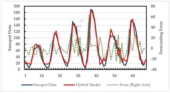
Figure 4.
Hybrid forecast vs. actual data over the test data (sunspot data—67 observations).

Table 1.
Comparison of forecast performance over test data for sunspot data.
4.2. Canadian Lynx Trapping
This series includes Canadian lynx trapped in Northwest Canada from 1821 to 1934. The lynx population has cyclical behavior over a period of 10 years. It is reported that this interesting cycle is observable for other animal populations in North Canada [27]. The cyclical behavior has tall peaks and deep bottoms, making it a challenging series for forecasting. The first 100 observations, data from 1821 to 1920, are used as the training set. The test section covers observations from 1921 to 1934, with 14 data points. Based on previous research on this problem, an AR(12) model is used in the basic model. An ANN architecture of 7 × 5 × 1 is selected for the secondary model.
Figure 5 shows the fitted values versus the actual data. The forecast performance in comparison to other models is presented in Table 2. Although the proposed model performed better than Zhang’s, the performance is slightly lower, or on par, compared to the others.
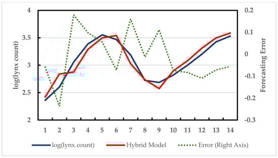
Figure 5.
Hybrid forecast vs. actual data over the test data (Canadian lynx—14 observations).
Table 2.
Comparison of forecast performance over test data for Canadian lynx data.
4.3. Hourly Electricity Rates
This data set includes hourly electricity prices in the New South Wales State of Australia. The price data are kept by the Australian Energy Market Operator (AEMO), a semi-official organization in charge of Australia’s national electricity and gas markets [35]. Price statistics for March 2013 are analyzed in this study. In the original data set, the price is recorded at half-hour intervals. First, the data set is converted to hourly rates with 24 records per day, totaling 744 (31 × 24) data points for the entire month (i.e., March 2013). While the first 30 days of data are used for development, the last day of the month is reserved as test data. ARIMA (1,0,1) and a multi-layer perceptron type of ANN architecture of 7 × 6 × 1 are used in basic and secondary models. Figure 6 shows the fitted versus actuals for the 24 h period of 31 March 2013. Table 3 includes MSE and MAD comparisons. Error statistics suggest that the proposed approach performed relatively better than benchmarks in terms of both metrics.
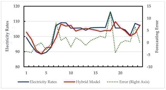
Figure 6.
Hybrid forecast vs. actual data over the test data (hourly electricity rates—24 observations).
Table 3.
Comparison of forecast performance over test data (hourly electricity rates).
4.4. Airline Passenger Data
This is popular time-series data, including monthly international passenger counts from 1949 to 1960. Since its introduction by Brown [28], this series has been the subject of many studies, and it is a popular benchmark for forecasting models. The series is readily available in data repositories and statistical software libraries [36]. There is a clear seasonality and an upward trend in the data, making it an exemplary test case for any time series modeling (Figure 7). The twelve-year monthly series has 144 observations. In our analysis, the first 11 years of the data (1949 to 1959) are used as a training set, while the remaining 12 observations of 1960 are used for testing.
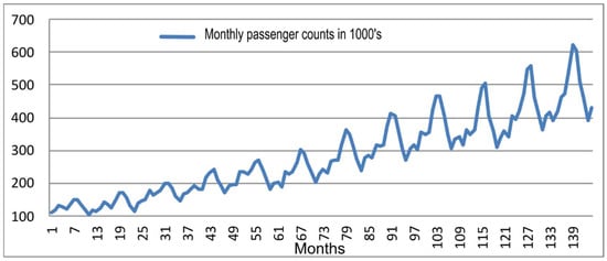
Figure 7.
Monthly airline passenger data.
For this data set, we used SARIMA (0,1,1) × (0,1,1)12 in the basic model. This representation was first used by Box et al. [37]. Because of the exponential upward trend, a logarithmic transformation is applied beforehand. The model originally proposed by Box et al. [37] is also confirmed by later studies [38,39]. For ANN in the secondary model, the input includes three nodes with lags 1, 2, and 12. There are two nodes in the hidden layer and a single output. Our basic model is based on the SARIMA (i.e., seasonal ARIMA) architecture, as proposed by [39].
The output of the hybrid model on the test data covering 12 months of 1960 is shown in Figure 8. In addition, the performance comparison with respect to two previous studies is presented in Table 4. Although the model performed significantly better than one of the comparisons [38] in MSE metrics, its performance was slightly worse in the second one [39]. It is worth mentioning that our model performed marginally better on MDA metrics.
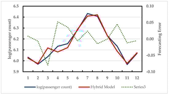
Figure 8.
Hybrid forecast vs. actual data over the test data (airline passenger data).
Table 4.
Comparison of forecast performance over test data (airline passenger data).
4.5. Wheat Yield in Turkey
This data set is about wheat yields in Turkey. The yield refers to the dry grain of the harvested crop, and it is often expressed in terms of either kilograms per decare or tons per hectare. The yield data are in an annual series, covering the period from 1938 to 2013. Turkey is a major wheat producer and a leading trader of cereals, including wheat. Because of the strategic importance of the crop, speculations regarding wheat yield are a great concern for many parties, particularly those involved in commodities trading. Although wheat is considered a strategic agricultural commodity in Turkey, the output has been flat for years. The decline in land dedicated to wheat agriculture has been partially compensated by an increase in yields, which kept the output at a level of 20 million tons per year [40]. For agricultural commodities such as wheat, yield is defined in terms of kilograms of seeds harvested per decare (1000 m2). As a first step in model development, the available data set was split into development and test sections, with 80% and 20% ratios. Yield data from 1938 to 1998 were used for model development, and the remaining portion, data from 1999 to 2013, was used for testing.
Historical change in yields from 1938 to 2013 is given in Figure 9. As the graph shows, the wheat yield in Turkey has been rising in recent years, but it is still well below the major wheat producers of Europe, such as Germany or France [41,42]. The yield data have an upward trend with random fluctuations. It does not exhibit any seasonal or periodic variations. For basic and secondary models, ARIMA (0,1,0) time series and an ANN architecture of 7 × 7 × 1 are selected as final models after testing various combinations.
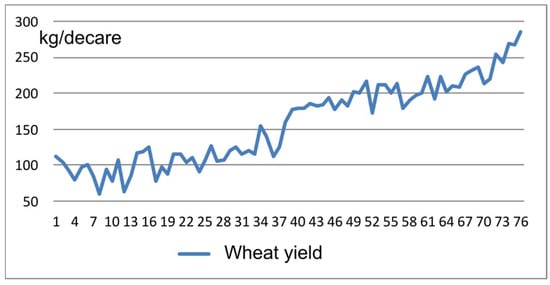
Figure 9.
Historical wheat yield in Turkey.
The graph of fitted values versus actuals for the test data (from 1999 to 2013) shows that the model captures the recent upward trend with reasonable accuracy (Figure 10). Performance statistics (MSE, MAD, and MAPE) for the hybrid model are given in Table 5. This table includes statistics for two more models. Two sub-components of the hybrid approach, the ARIMA model in the basic model and the ANN model in the secondary models, are run separately on the yield data. The performance of each model is recorded, and relevant error metrics are included in Table 5.
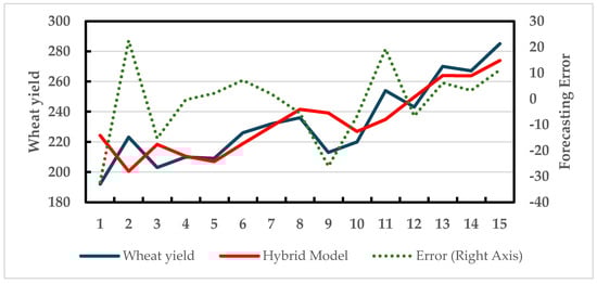
Figure 10.
Hybrid forecast vs. actual data over the test data (wheat yield).
Table 5.
Comparison of forecast performance over test data (wheat yield data).
4.6. Ablation Study
As part of the design process, we tested each component separately on five data sets. This helps us evaluate each component’s specific effectiveness in the hierarchy. Table 6 lists the performance of ARIMA and ANN models, along with the proposed hybrid one. For all five data sets, the performance of the hybrid model is better than that of individual ARIMA and ANN models in terms of MSE and MAD metrics. However, the performance gap varies significantly from one data set to another. In two data sets, namely, hourly electricity rates and wheat yield, hybrid forecasting has superior performance over ARIMA and ANN. In other data sets, the gap between the hybrid model and ANN is relatively small.
Table 6.
Ablation study of test data sets.
5. Conclusions
Previous research has shown that combining different forecasting methods in a framework generates superior results to stand-alone models based on a single methodology. The last case (i.e., yield forecasting) presented in the “Experimental Results” section clearly illustrates this phenomenon. For that case, we first run the ARIMA and ANN models separately. Then, we run the hybrid model that combines ARIMA and ANN in a unique framework. Accuracy metrics in Table 5 show that the hybrid model’s performance is far superior to stand-alone ARIMA or stand-alone ANN. Combining different forecasting methods in a framework has been previously studied by many researchers, and different approaches have been proposed. Our approach is an improvement along this line of research. As we detailed in the previous section, the performance in terms of forecast accuracy has been better than, or on par with, similar approaches.
In terms of future work, there are several potential areas in which this research can be extended. From a methodology perspective, alternative approaches can be used to capture both linear and nonlinear patterns in the data. In our literature review, we mentioned some of the methods already used by other researchers. However, there are always opportunities to explore new alternatives. Another extension to this research is to include more real-life data for testing.
Author Contributions
Conceptualization, M.G. and A.A.; methodology, M.G. and A.A.; validation, A.A.; formal analysis, M.G. and A.A.; investigation, M.G. and A.A.; resources, M.G. and A.A.; data curation, A.A.; writing—original draft preparation, A.A.; writing—review and editing, M.G. and A.A.; visualization, M.G. and A.A.; supervision, M.G. All authors have read and agreed to the published version of the manuscript.
Funding
This research received no external funding.
Institutional Review Board Statement
Not applicable.
Informed Consent Statement
Not applicable.
Data Availability Statement
The original data presented in the study are openly available in FigShare at 10.6084/m9.figshare.26113714.
Conflicts of Interest
The authors declare no conflicts of interest.
References
- Tsay, R.S.; Chen, R. Nonlinear Time Series Analysis; John Wiley & Sons: Hoboken, NJ, USA, 2018; ISBN 978-1-119-26405-7. [Google Scholar]
- Bates, J.M.; Granger, C.W.J. The Combination of Forecasts. Oper. Res. Q. 1969, 20, 19. [Google Scholar] [CrossRef]
- Smyl, S. A Hybrid Method of Exponential Smoothing and Recurrent Neural Networks for Time Series Forecasting. Int. J. Forecast. 2020, 36, 75–85. [Google Scholar] [CrossRef]
- Makridakis, S.; Hibon, M. The M3-Competition: Results, Conclusions and Implications. Int. J. Forecast. 2000, 16, 451–476. [Google Scholar] [CrossRef]
- Zhang, G.P. Time Series Forecasting Using a Hybrid ARIMA and Neural Network Model. Neurocomputing 2003, 50, 159–175. [Google Scholar] [CrossRef]
- Khashei, M.; Bijari, M. An Artificial Neural Network (p,d,q) Model for Timeseries Forecasting. Expert Syst. Appl. 2010, 37, 479–489. [Google Scholar] [CrossRef]
- Banihabib, M.E.; Ahmadian, A.; Valipour, M. Hybrid MARMA-NARX Model for Flow Forecasting Based on the Large-Scale Climate Signals, Sea-Surface Temperatures, and Rainfall. Hydrol. Res. 2018, 49, 1788–1803. [Google Scholar] [CrossRef]
- do Nascimento Camelo, H.; Lucio, P.S.; Junior, J.B.V.L.; de Carvalho, P.C.M.; dos Santos, D.V.G. Innovative Hybrid Models for Forecasting Time Series Applied in Wind Generation Based on the Combination of Time Series Models with Artificial Neural Networks. Energy 2018, 151, 347–357. [Google Scholar] [CrossRef]
- Farajzadeh, J.; Alizadeh, F. A Hybrid Linear-Nonlinear Approach to Predict the Monthly Rainfall over the Urmia Lake Watershed Using Wavelet-SARIMAX-LSSVM Conjugated Model. J. Hydroinform. 2018, 20, 246–262. [Google Scholar] [CrossRef]
- Moeeni, H.; Bonakdari, H. Impact of Normalization and Input on ARMAX-ANN Model Performance in Suspended Sediment Load Prediction. Water Resour. Manag. 2018, 32, 845–863. [Google Scholar] [CrossRef]
- Buyuksahin, U.C.; Ertekina, S. Improving Forecasting Accuracy of Time Series Data Using a New ARIMA-ANN Hybrid Method and Empirical Mode Decomposition. Neurocomputing 2019, 361, 151–163. [Google Scholar] [CrossRef]
- Chakraborty, T.; Chattopadhyay, S.; Ghosh, I. Forecasting Dengue Epidemics Using a Hybrid Methodology. Phys. A-Stat. Mech. Its Appl. 2019, 527, 121266. [Google Scholar] [CrossRef]
- Safari, A.; Davallou, M. Oil Price Forecasting Using a Hybrid Model. Energy 2018, 148, 49–58. [Google Scholar] [CrossRef]
- Song, M.; Wang, R.; Li, Y. Hybrid Time Series Interval Prediction by Granular Neural Network and ARIMA. Granul. Comput. 2024, 9, 3. [Google Scholar] [CrossRef]
- Aasim; Singh, S.N.; Mohapatra, A. Repeated Wavelet Transform Based ARIMA Model for Very Short-Term Wind Speed Forecasting. Renew. Energy 2019, 136, 758–768. [Google Scholar] [CrossRef]
- Liu, H.-H.; Chang, L.-C.; Li, C.-W.; Yang, C.-H. Particle Swarm Optimization-Based Support Vector Regression for Tourist Arrivals Forecasting. Comput. Intell. Neurosci. 2018, 2018, 6076475. [Google Scholar] [CrossRef]
- Madan, R.; Mangipudi, P.S. Predicting Computer Network Traffic: A Time Series Forecasting Approach Using DWT, ARIMA and RNN. In Proceedings of the 2018 Eleventh International Conference on Contemporary Computing (ic3), Noida, India, 2–4 August 2018; Aluru, S., Kalyanaraman, A., Bera, D., Kothapalli, K., Abramson, D., Altintas, I., Bhowmick, S., Govindaraju, M., Sarangi, S.R., Prasad, S., et al., Eds.; IEEE: New York, NY, USA, 2018; pp. 1–5, ISBN 978-1-5386-6835-1. [Google Scholar]
- Çağlayan-Akay, E.; Topal, K.H. Forecasting Turkish Electricity Consumption: A Critical Analysis of Single and Hybrid Models. Energy 2024, 305, 132115. [Google Scholar] [CrossRef]
- Siqueira-Filho, E.A.; Lira, M.F.A.; Siqueira, H.V.; Bastos-Filho, C.J.A. Multivariate and Hybrid Data-Driven Models to Predict Thermoelectric Power Plants Fuel Consumption. Expert Syst. Appl. 2024, 252, 124219. [Google Scholar] [CrossRef]
- Zhang, J.; Liu, H.; Bai, W.; Li, X. A Hybrid Approach of Wavelet Transform, ARIMA and LSTM Model for the Share Price Index Futures Forecasting. N. Am. J. Econ. Financ. 2024, 69, 102022. [Google Scholar] [CrossRef]
- Dos Santos de Jesus, E.; Silva Gomes, G.S. da Machine Learning Models for Forecasting Water Demand for the Metropolitan Region of Salvador, Bahia. Neural Comput. Appl. 2023, 35, 19669–19683. [Google Scholar] [CrossRef]
- Babu, C.N.; Reddy, B.E. A Moving-Average Filter Based Hybrid ARIMA–ANN Model for Forecasting Time Series Data. Appl. Soft Comput. 2014, 23, 27–38. [Google Scholar] [CrossRef]
- Hyndman, R.J.; Koehler, A.B. Another Look at Measures of Forecast Accuracy. Int. J. Forecast. 2006, 22, 679–688. [Google Scholar] [CrossRef]
- Makridakis, S.G.; Wheelwright, S.C.; Hyndman, R.J. Forecasting: Methods and Applications; Wiley: Hoboken, NJ, USA, 1998; ISBN 978-0-471-53233-0. [Google Scholar]
- Khashei, M.; Bijari, M.; Raissi Ardali, G.A. Hybridization of Autoregressive Integrated Moving Average (ARIMA) with Probabilistic Neural Networks (PNNs). Comput. Ind. Eng. 2012, 63, 37–45. [Google Scholar] [CrossRef]
- Sunspot Number|SILSO. Available online: http://www.sidc.be/silso/datafiles (accessed on 10 March 2021).
- Bulmer, M.G. A Statistical Analysis of the 10-Year Cycle in Canada. J. Anim. Ecol. 1974, 43, 701–718. [Google Scholar] [CrossRef]
- Brown, R.G. Smoothing, Forecasting and Prediction of Discrete Time Series; Prentice Hall: Englewood Cliffs, NJ, USA, 1962. [Google Scholar]
- Turkish Grain Board TMO—Turkish Grain Board Statistics. Available online: https://www.tmo.gov.tr/bilgi-merkezi/tablolar (accessed on 5 June 2021).
- The Sun—History. Available online: https://pwg.gsfc.nasa.gov/Education/whsun.html (accessed on 10 March 2021).
- Inzenman, A.J.; Wolf, J.R.; Wolfer, H.A. An Historical Note on the Zurich Sunspot Relative Numbers. J. R. Stat. Soc. Ser. A 1983, 146, 311–318. [Google Scholar] [CrossRef]
- Suyal, V.; Prasad, A.; Singh, H.P. Nonlinear Time Series Analysis of Sunspot Data. Sol. Phys. 2009, 260, 441–449. [Google Scholar] [CrossRef][Green Version]
- Cottrell, M.; Girard, B.; Girard, Y.; Mangeas, M.; Muller, C. Neural Modeling for Time Series: A Statistical Stepwise Method for Weight Elimination. IEEE Trans. Neural Netw. 1995, 6, 1355–1364. [Google Scholar] [CrossRef] [PubMed]
- Rao, T.S.; Gabr, M.M. An Introduction to Bispectral Analysis and Bilinear Time Series Models; Springer Science & Business Media: Berlin/Heidelberg, Germany, 2012; ISBN 978-1-4684-6318-7. [Google Scholar]
- Australian Energy Market Operator. Available online: https://aemo.com.au/ (accessed on 13 June 2024).
- R-Manual R: Monthly Airline Passenger Numbers 1949–1960. Available online: https://stat.ethz.ch/R-manual/R-patched/library/datasets/html/AirPassengers.html (accessed on 25 March 2021).
- Box, G.E.P.; Jenkins, G.M.; Reinsel, G.C.; Ljung, G.M. Time Series Analysis: Forecasting and Control, 5th ed.; Wiley: Hoboken, NJ, USA, 2015; ISBN 978-1-118-67502-1. [Google Scholar]
- Faraway, J.; Chatfield, C. Time Series Forecasting with Neural Networks: A Comparative Study Using the Air Line Data. J. R. Stat. Soc. Ser. C (Appl. Stat.) 1998, 47, 231–250. [Google Scholar] [CrossRef]
- Hamzaçebi, C. Improving Artificial Neural Networks’ Performance in Seasonal Time Series Forecasting. Inf. Sci. 2008, 178, 4550–4559. [Google Scholar] [CrossRef]
- Dunya, Economic Daily Decline in Land Use for Startegic Commodity, Wheat. Available online: https://www.ekonomim.com/sehirler/stratejik-urun-bugday-ekim-alanlari-daraliyor-haberi-470018 (accessed on 3 May 2021).
- World Bank Cereal Production (Metric Tons)|Data. Available online: https://data.worldbank.org/indicator/AG.PRD.CREL.MT (accessed on 22 March 2021).
- Tİryakİoğlu, M.; Demİrtaș, B.; Tutar, H. Comparison of Wheat Yield in Turkey: Hatay and Şanlıurfa Study Case. Süleyman Demirel Univ. Ziraat Fakültesi Derg. 2017, 12, 56–67. [Google Scholar]


Disclaimer/Publisher’s Note: The statements, opinions and data contained in all publications are solely those of the individual author(s) and contributor(s) and not of MDPI and/or the editor(s). MDPI and/or the editor(s) disclaim responsibility for any injury to people or property resulting from any ideas, methods, instructions or products referred to in the content. |
© 2024 by the authors. Licensee MDPI, Basel, Switzerland. This article is an open access article distributed under the terms and conditions of the Creative Commons Attribution (CC BY) license (https://creativecommons.org/licenses/by/4.0/).