Abstract
The probing depth of the transient electromagnetic method (TEM) refers to the depth range at which the underground conductivity changes can be effectively detected. It typically ranges from tens of meters to several kilometers and is influenced by factors such as instrument parameters and the conductivity of the subsurface structure. Rapid and accurate probing depth is useful for the selection of appropriate inversion parameters and improving survey accuracy. However, mainstream methods suffer from issues such as low computational precision, large uncertainties, or high computational requirements, making them unsuitable for processing massive airborne electromagnetic data. In this study, we propose a prediction model based on deep learning that can directly compute the probing depth from the TEM responses, and its effectiveness and accuracy are validated through synthetic models and field measurements. We compared the performance of classic deep learning models, including CNN, RESNET, and RNN, and found that RNN performed the best overall on both synthetic and field data. Furthermore, we apply this algorithm to deep learning-based ATEM inversion by constraining the one-dimensional resistivity model depths in the training set, to reduce the non-uniqueness of the inversion, accelerate the convergence, and improve its prediction accuracy.
1. Introduction
In the realm of geophysical electromagnetic imaging methods, including ground and airborne transient electromagnetic surveys, as well as frequency domain electromagnetic methods, probing depth (or skin depth) has always been one of the most crucial parameters of interest for exploration geophysicists. It not only characterizes the confidence region of the inversion model but also serves as an evaluation criterion for the adequacy of instrument settings. The transient electromagnetic method (TEM) is a technique that utilizes electromagnetic induction to investigate the internal structure, rock properties, and natural environment of the earth [1,2]. Unlike seismic exploration or ground-penetrating radar methods, which are based on wave equations [3], in transient electromagnetic or frequency domain electromagnetic methods, the propagation of low-frequency electromagnetic fields in subsurface media follows the diffusion equation. For wave equation problems, the effective signal’s range can be inferred by observing the wave impedance interface of the received signal, such as seismic exploration. However, for diffusion equation problems, it is difficult to determine the range of influence of the effective signal directly from the observations. As a result, it is challenging to directly obtain the probing depth from the TEM measurements.
Currently, there are two mainstream methods for estimating the probing depth in the TEM. The first method assumes a uniform half-space medium with planar electromagnetic wave incidence to approximate the relationship between the latest cut-off time and the probing depth [4,5,6,7]. However, this approach does not sufficiently consider the effects of non-uniform resistivity structures and the number of sampling points. It relies on reasonable estimates of the half-space model, which introduces considerable uncertainty. The second method involves calculating the probing depth based on the Jacobian matrix derived from the inversion model [8]. This method allows for the calculation of probing depth for any model and takes into account the influences of noise and the number of sampling points. However, the second approach requires the availability of a well-defined inversion model, which itself depends on the predetermined probing depth. Additionally, the inversion process is inherently subject to non-uniqueness and affected by various parameters, leading to potential errors. Moreover, for large-scale datasets, such as airborne transient electromagnetic data, the Jacobian-matrix-based method entails a significant computational burden, making it unsuitable for real-time data processing [9]. A better approach is to directly calculate the probing depth based on the transient electromagnetic curve. To date, there is currently no developed algorithm for this purpose, but it is theoretically feasible since the probing depth depends on the resistivity model, which directly influences the observed data.
In recent years, several studies have successfully applied deep learning (DL) algorithms to the one-dimensional inversion of ATEM [10,11,12]. These studies attempt to construct a “fully mapping” inversion operator that directly transforms observed data into predicted models [9,10,13,14,15] by minimizing the loss function of the predicted model based on the training data to obtain data-driven trained models [16,17]. The training process allows neural network algorithms to abstract high-dimensional feature maps and learns complex mapping functions, thereby avoiding issues associated with linearized inversion, such as convergence to local minima.
This study firstly proposes a new method for estimating TEM probing depth based on deep learning models. The method takes the cut-off time and induced electromotive force (IEF) as inputs and the probability distribution of the probing depth as output. It establishes a direct predictive model from the measurements to the probing depth, eliminating the need for inversion calculations and sensitivity matrix estimation. This approach reduces the subjective influence of manually setting involved parameters and improves the computational efficiency of the probing depth calculation. The open-source Python code can be obtained from the following GitHub repository: https://github.com/Rongjiang007/TEM-probing-Depth-prediciton (accessed on 14 July 2024). The proposed method is further applied to deep-learning-based airborne TEM inversion by constraining the probing depth of one-dimensional resistivity models. This approach aims to enhance the predictive capability of the neural network and strengthen the correlation between the input data and the predictions.
2. The Calculation of the TEM Probing Depth
In this chapter, we present the conventional methods for probing depth estimation, aiming to facilitate a comparison with deep-learning-based prediction algorithms. Additionally, we will utilize these methods to obtain labels for the dataset, which will guide the training of the network mode.
The traditional methods for calculating probing depth mainly involve two approaches. The first approach directly calculates the probing depth using the following theoretical formula [18]:
where t represents the cut-off time, μ denotes magnetic permeability, and σ represents the electrical conductivity of the half-space model. This approach has significant uncertainty because it fails to fully consider the non-uniform conductivity structure and the influence of the number of sampling points. Moreover, it relies on a reasonable estimation of the half-space model.
Another approach is the Jacobian-matrix-based calculation method proposed by Christiansen and Auken (2012) [19]. It is generally obtained through the following steps: (1) Perform one-dimensional inversion on the measured data. (2) Interpolate the one-dimensional inversion model to obtain a multi-layer model with thin layer thickness. (3) Calculate for the interpolated model using , where represents the value of the i-th data points and the represents the value of the j-th layer in the inversion model. (4) Calculate using and consider the depth where equals 0.8 as the probing depth; here the is noise on the data points. However, this method is highly dependent on the inversion results, which themselves have uncertainty due to the non-uniqueness of the inversion solution. Additionally, the computational efficiency of this method is low when dealing with large amounts of data.
3. Deep Learning Model and Training
We propose a residual neural network for rapid estimation of the probing depth from TEM data. The performance of deep learning models is greatly influenced by the training datasets; thus, a large number of the subsurface resistivity models and the corresponding TEM responses are often required. We chose a public standard benchmark database from Asif et al. (2022) [20], and this database includes 1 million geologically plausible models and EM resolvable 1-D subsurface resistivity models spanning the resistivity range from 1 Ωm to 2000 Ωm and a depth of 500 m, which is suitable for ground-based and airborne EM systems in a DL context. Here we select a sub-dataset with an intermediate depth of 350 m which consists of 137,000 one-dimensional resistivity models.
The vertical-induced electromotive force responses for these models are computed using 1D layered model analytical solutions [9], and the probing depths for each model are calculated using the sensitivity matrix obtained through a 1D electromagnetic field [19]. The training dataset comprises 90,000 samples, while the remaining 10,000 samples are allocated for testing purposes. Simulated TEM responses serve as the input to the neural network, and the computed probing depths are utilized as the network’s output.
Then, three deep learning models are constructed as shown in Figure 1. CNN (Convolutional Neural Network) is a deep learning model designed for processing data with a grid-like topology, such as images. It primarily consists of convolutional layers that apply filters to extract local features from the input, pooling layers that reduce the spatial dimensions of the feature maps, and fully connected layers that perform classification or regression tasks. RESNET (Residual Network) is a type of deep neural network that addresses the challenges of training very deep networks by incorporating residual blocks. These blocks use shortcut connections to skip one or more layers, allowing gradients to flow more easily through the network and mitigating issues like vanishing and exploding gradients [21]. RNN (Recurrent Neural Network) is a type of neural network designed for sequential data, where connections between nodes can create a cycle, allowing information to persist. RNNs are particularly useful for tasks involving time series or natural language, as they can capture temporal dependencies and patterns in sequences. LSTM (Long Short-Term Memory) is a specialized type of RNN (Recurrent Neural Network) [22] designed to address some of the limitations of traditional RNNs, particularly the vanishing and exploding gradient problems. LSTMs are well-suited for learning long-term dependencies in sequential data.
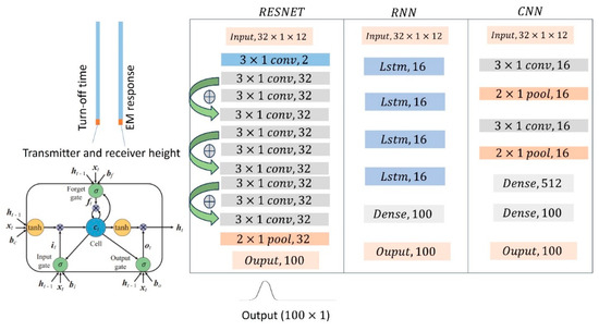
Figure 1.
The RESNET, RNN, and CNN framework used for prediction of probing depth and schematic input representation. The sizes and numbers of convolutional or pooling kernels are indicated within each layer, with green arrows representing shortcut connections. The lower-left subfigure shows a long short-term memory (LSTM) block containing a memory cell and the input, output, and forget gates (modified from Gers et al., 2000 [22]).
The input of the DL models consists of two channels: the cut-off time and the induced electromotive force (IEF). We take the logarithm of the input to reduce the magnitude difference of the IEF [23]. The last neuron of each channel represents the heights of the transmitter and receiver coils. The final input data shape is 32 × 2, where each channel contains 62 neurons for the cut-off time and electromotive force data, and 2 neurons for the height data. Observation elevations of receiving are randomly set to be uniformly distributed in the range [0, 30] m, and the height of the transmitting coil is 10~30 m higher than that of the receiving coil. The number of sampling points is variable and distributed uniformly between 20 and 31. The cut-off time points are distributed logarithmically between the earliest and latest shut-off times, and the earliest and latest cut-off times are also variable, following a logarithmic uniform distribution: , , respectively.
The output is a Gaussian distribution with a size of 100 × 1 representing the probing depth [24]. The maximum probing depth is set to 350 m, which depends on the scale of the models in the training dataset. The peak of the Gaussian distribution corresponds to the predicted depth. The network consists of a total of 8 layers, including 7 convolutional layers and 1 pooling layer. The RELU activation function is used in every convolutional layer to improve the nonlinear ability of the network and reduce the likelihood of the vanishing gradient. Furthermore, the sigmoid function is applied to the last convolution layer to limit the output value within the range of [0, 1]. The loss function is defined using binary cross-entropy between the true probability distribution and prediction distribution [16,25]:
Here, , , and represents the abscissa of the output distribution. Cross-entropy naturally fits with probabilistic outputs, as it directly measures the difference between the predicted probability distribution and the true distribution. The loss decreases as the predicted probabilities get closer to the true labels [25].
Three models are trained using the same dataset. The inputs, outputs, and hyperparameters of the different models are completely identical for comparison. The model’s learning rate was set to 0.001, the batch size to 200, and the number of iterations to 200. Other parameters, including the kernel size, number of convolutional layers, and pooling size, are referenced in Figure 1. The model parameters of the ResNet are continuously updated through backpropagation algorithm Adam [26]. Each model was trained using a GPU (NVIDIA GeForce RTX 3070, NVIDIA Corporation, Santa Clara, CA, USA) of desktop workstation (Processor: 12th Gen Intel(R) Core(TM) i9-12900K 3.20 GHz, Memory: 128 GB, Intel Corporation, Santa Clara, CA, USA), with the 200 epoch training process taking approximately 20 min. After training, the prediction time for 10,000 measuring data is within 1 s. In a set of 137,000 geoelectrical models, 90% are used for training, and 10% are used as a test dataset to evaluate the model’s performance on unseen data. Figure S1 presents the evolution of the loss function during the training process. It can be observed that the errors of both the training and testing sets gradually decrease with increasing iteration numbers and eventually reach a stable state. This indicates that the model successfully learns the features present in the training set.
In addition, we further investigate the relationship between probing depth and observed data to demonstrate the effectiveness of the algorithm (Figure 2). The late-time IEF [8] is not only associated with the cut-off time controlling the slope of the decay curve but also serves as a comprehensive reflection of subsurface rock resistivity. Figure 2b,c represent the relationship between labeled depth and predicted depth with the IEF at the last cut-off moment, respectively. As the late-time IEF decreases (represented by negative values after taking the logarithm, thus larger values on the x-axis indicating smaller IEF), the probing depth gradually increases. This is because a faster decay of the electromagnetic field indicates higher resistivity, leading to greater penetration depth of the electromagnetic field. The significant similarity observed in Figure 2b,c demonstrates that the deep learning model can effectively learn the mapping relationship between the induced electromotive force curve and the probing depth.
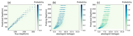
Figure 2.
Prediction of testing dataset. (a) Joint distributions of label and prediction. (b) Joint distributions of label and late-time IEF. (c) Joint distributions of prediction and the late-time IEF.
4. Synthetic Data Test
To evaluate the performance of the proposed algorithm, taking RESNET as an example, we designed two synthetic models as shown in Figure 3. The differences between the two models lie in the distinct electrical resistivity contrasts at a depth of 100 m and in local regions near the Earth’s surface. In model I, the probing depth on the left side is limited due to the shielding effect of the conductivity layer. Conventional algorithms are affected by inversion model discrepancies near the shallow low-velocity zone (Figure S2), whereas the predictions of deep learning models closely resemble the probing depth derived from the true model. The true model is derived from one-dimensional slices, thus exhibiting abrupt changes in probing depth in localized areas devoid of conductivity layers. The uncertainty of the 1D inverted model near the surface may result in reduced probing depth (Figure S2). Such discrepancies are also governed by different inversion parameters, such as regularization parameters.
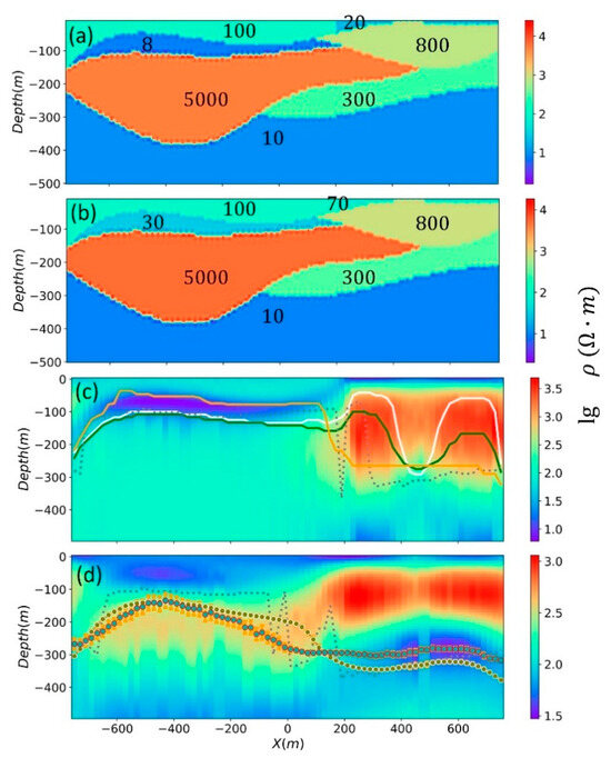
Figure 3.
(a) Model I. The numbers indicate resistivity (Ωm). (b) Model II. (c) The probing depth derived from the 1D inverted model I (white with regularization parameter 0.2 and green curves with 1.0). Dotted and orange curves show the probing depth derived from true model and ResNet. (d) The brown points show the probing depth derived from the 100 1D inverted model II, which are obtained from 100 synthetic IEFs with 10% random Gaussian noise. The background model was obtained from a noise-free 1D inversion. The cyan points show the probing depth derived from ResNet using the same 100 synthetic IEFs with 10% random Gaussian noise. The vertical orange line length on each scatter point represents the standard deviation.
In model II, when the shallow low-velocity layer is absent, the probing depths obtained by both deep learning and conventional methods closely align. To test the noise resilience of different algorithms, we introduced random Gaussian noise of 10% to the synthetic observations. This process was repeated 100 times for probing depth prediction. Interestingly, conventional algorithms demonstrated superior noise resistance. However, despite this, the prediction deviations of deep learning remained within an acceptable range. The uncertainty introduced by the conventional inverted model led to discrepancies in prediction far exceeding the uncertainty introduced by noise. These results demonstrate the effectiveness of the DL predictions. We also found that ResNet demonstrates good noise resistance when trained with noisy data (Figure S3).
In Table 1, we compared the performance of different deep learning models by evaluating the test dataset’s Mean Absolute Error (MAE), Mean Absolute Percentage Error (MAPE), Root Mean Square Error (RMSE), as well as cross-entropy loss. The loss evolution curves of the three functions are shown in Figure S1. Overall, all three models performed well, with RNN performing the best and RESNET performing relatively worse.

Table 1.
Performance of different deep learning models on test datasets.
5. Field Example
To investigate the practical applicability of the algorithm proposed in this study, airborne transient electromagnetic data collected by the United States Geological Survey (USGS) in Leach Lake Basin, California, Fort Irwin, were utilized for testing (http://dx.doi.org/10.3133/ofr20131024G). The survey area is a geologically complex, internally drained basin bisected and flanked by a number of faults, as shown in Figure 4.
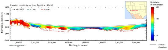
Figure 4.
Probing depth prediction of field data using different DL models. The map shows the location of the study area at Fort Irwin, California, USA. The resistivity section along line L10450 is gained by stitching together the 1-D models obtained from Bedrosian et al. (2014) [27]. The black, green, and red dots represent the probing depth predicted by the ResNet, CNN, and RNN, respectively.
Inverting a large volume of AEM data and calculating probing depth is very time-consuming by conventional inversion techniques. A conventional 1D inversion and Jacobian matrix computation typically require around 20 to 30 s for a single TEM measurement. Using well-trained ResNet in our study, however, it takes less than 2 s to obtain over 2000 probing depth estimations. This is of great significance for handling a large volume of field-measured airborne TEM data. The inversion profile in Figure 4 is from Bedrosian et al. (2014) [27], and the probing depth is obtained through the inversion model. The dots in the profile represent the probing depth predicted by the DL models. The variation trends of the predicted probing depth by the three DL models are generally consistent with the probing depth calculated through the inverted model. Specifically, in areas with lower overall resistivity, the predicted probing depth is shallow, while in areas with higher overall resistivity, the predicted probing depth is greater. This alignment confirms the effectiveness of the DL models in predicting the probing depth based on the field airborne transient electromagnetic measurements.
The predictions from RNN and RESNET are essentially overlapping, while the depth predicted by CNN is relatively shallower. Since the predictions from RNN and RESNET are closer to the traditional methods, we believe that RNN and RESNET better capture the nonlinear relationship between the observations and probing depth, resulting in superior prediction performance. This is particularly interesting; although RESNET does not seem to outperform CNN on the test set (Table 1, Figure S1), it exhibits better generalization ability on field data. In general, RNN performed the best overall on both synthetic and field data. Due to the more complex architectures of the RNN and RESNET models compared to CNN, these findings suggest that advanced models have an advantage in data transferability.
6. Discussion
Recently, several research studies have successfully applied deep learning algorithms to one-dimensional transient electromagnetic (TEM) rapid inversion [9,10,11,12]. Despite achieving encouraging progress, most of these studies have primarily focused on neural network structure and data preprocessing, with less discussion on how to set up a reasonable training dataset. As a data-driven approach, deep learning algorithms heavily rely on the rationality of the training dataset. The design of the training dataset not only needs to cover as many underground structures as possible but also needs to comply with the characteristics of the geophysical field itself. For instance, if the resistivity models in the training dataset exceed the resolution of the TEM method, the neural network cannot identify high-resolution structures from the corresponding observed data. As a result, the loss function may not decrease adequately, leading to a decline in prediction capability. Similarly, for certain low-resistivity models, the probing depth of TEM is limited and may not be sufficient to identify structures below the probing depth. In such cases, the neural network also fails to provide accurate predictions. Conventional inversion methods for TEM typically employ regularization algorithms [28,29] (Tikhonov and Arsenin, 1977; Byrd et al., 1995), which means that models without resolution are mainly determined by the regularization smooth term in the objective function. However, neural networks do not possess this characteristic, resulting in weaker prediction capability below the probing depth.
To address this issue, we utilize the proposed rapid prediction algorithm to constrain the probing depth of the publicly available resistivity model repository from Asif et al. (2022) [20]. Then, we conduct TEM one-dimensional inversion based on UNet (Figure 5) for both the unconstrained and constrained model repositories, and compare the prediction results of the two to validate the effectiveness. As the TEM inversion problem requires a more advanced architecture than probing depth prediction to learn more complicated characteristics, we adapt the prevalent CNN-based UNet [30] architecture to directly learn the mapping from input (TEM response) to output (Resistivity model). The input data structure of UNet in Figure 5 is completely identical to that of ResNet in Figure 1, which means UNet is capable of handling various data of ground and airborne transient electromagnetics, including different cut-off times and different numbers of sampling points. We employ two types of processing for the output data labels: ① Datasets1: The resistivity models at a fixed depth of 350 m are obtained from the standard benchmark database. ② Datasets2: ResNet is utilized to predict the probing depth for each model in ①, and then the portion above the predicted detection depth is extracted as new labeled data. Additionally, a spline interpolation algorithm is employed to maintain the same number of layers as the original model, ensuring compatibility with the output dimensions of the neural network.
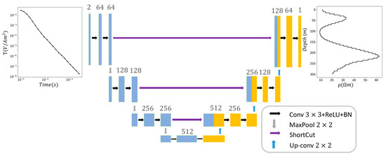
Figure 5.
UNet architecture for TEM model inversion. The model’s input is transient electromagnetic signals, and the output is the predicted subsurface resistivity. The black number above feature maps indicates the number of channels.
Then, two training sets are used to train two models, which are defined as and . Figure 6 illustrates the evolution of the loss function during the training process for the two training sets. It can be observed that the errors of both training sets gradually decrease and stabilize with increasing iterations, and the error curve of the constrained training set shows a greater reduction compared to the unconstrained training set. Similarly, compared to the training set, the overall trend of the error in the test set is similar, but the descent process is more unstable. Moreover, the error curve of the constrained testing dataset exhibits a greater and more stable reduction compared to the unconstrained testing dataset. This is because for models with shallow probing depths, the TEM response exhibits a weak correlation with deeper structures. In Datasets 2, the neural network no longer needs to fit these weakly correlated data, thereby improving its learning capacity for models with strong correlations. This indicates that is able to learn more effective features from the constrained training dataset.
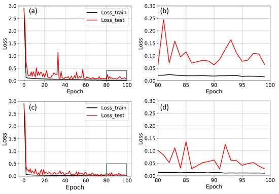
Figure 6.
The evolution of the loss functions for the training and testing sets during the training process. (a) shows the loss function curve for the unconstrained training set while Figure (b) is an enlarged view of the highlighted region in (a); (c) shows the loss function curve for the constrained training set while (d) is an enlarged view of the highlighted region in (c).
To demonstrate a more general pattern, we calculated the error distribution between 1000 predicted models and the corresponding true models in the two test datasets (Figure 7). It can be observed that the errors obtained from are mostly concentrated around zero but relatively dispersed. On the other hand, the errors obtained from are also distributed around zero but more concentrated, indicating a higher level of prediction accuracy compared to the former.
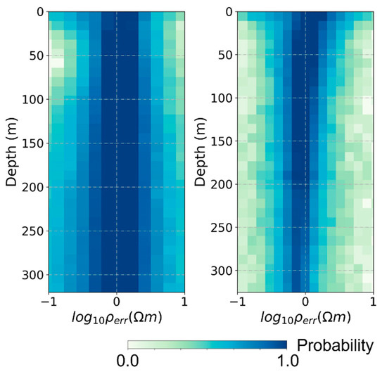
Figure 7.
The distribution of errors between the predictions and the true models for the two DL models (Left: , Right: ).
Figure 8 illustrates several examples illustrating the determination of the subsurface resistivity models from the test dataset. Some models obtained from the exhibit significant deviations from the true models in the deeper regions due to their shallower probing depth. On the other hand, the models obtained from the show better agreement with the true models. This indicates that by constraining the probing depth of the models, the network is able to better capture the mapping relationship between models and observed data, thereby enhancing the predictive capability of the neural network.
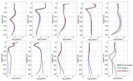
Figure 8.
Comparison of the predicted results and the true models for selected models in testing datasets.
7. Conclusions
We present a deep-learning-based method for rapidly estimating the probing depth of TEM. This method directly utilizes the IEF curve to obtain the probing depth, offering not only high efficiency but also avoiding the need for inversion calculations and the Jacobian matrices. We apply the algorithm to both theoretical models and field measurements, and the results demonstrate consistency with the decay pattern of the electromagnetic field. The method exhibits good accuracy and stability in estimating the probing depth. In addition, the trained ResNet can be flexibly applied to any scenarios with different cut-off times, sampling points, and flight altitudes, and is suitable for both airborne and ground transient electromagnetic observations. We also compared the predictions of three networks, including CNN, RESNET, and RNN, and found that RESNET and RNN had better prediction performance.
Furthermore, it reduces the subjective influence of manually setting involved parameters and improves the computational efficiency of the detection depth calculation, and avoids the probing depth estimation errors caused by the deviation in one-dimensional inversion, especially the surface conductivity layer (Figure 3c). This method can not only be used in time-domain EM; the same pattern can be easily transferred to the application of frequency-domain EM.
Accurate estimation of the detection depth is crucial for constructing a reasonable training dataset for inversion, as deep-learning-based inversion methods require a strong correlation between input data and predicted results. Therefore, we apply the algorithm to constrain the model depth in 1D inversions, aiming to reduce the non-uniqueness of the inversion and enhance the predictive capability of the deep learning model. This idea can be extended to the application of 2D and 3D inversion.
Supplementary Materials
The following supporting information can be downloaded at: https://www.mdpi.com/article/10.3390/app14167123/s1, Figure S1: The evolution of the loss functions for the training and testing datasets during the training process from different DL models; Figure S2: The 1D inverted model at 630 m for Model II (Figure 3) (left), with data misfit (right). The red box highlights the significantly lower surface resistivity of the inversion model compared to the true model, resulting in a reduction in probing depth; Figure S3: The probing depth derived from the 100 1D inverted model II. The curves are the same with Figure 3d except that the cyan points show the probing depth derived from ResNet trained without noisy training data.
Author Contributions
Conceptualization, L.G. and R.T.; methodology, L.G.; software, R.T.; validation, R.T. and F.S.; writing—original draft preparation, L.G.; writing—review and editing, L.G. and R.T.; visualization, F.S.; supervision, F.L.; funding acquisition, L.G. All authors have read and agreed to the published version of the manuscript.
Funding
This work is supported in part by Huzhou Public Welfare Research Project (2023GZ17), Basic Scientific Research Program from Yangtze Delta Region Institute (U032200109, U032200110).
Institutional Review Board Statement
Not applicable for studies not involving humans or animals.
Informed Consent Statement
Not applicable.
Data Availability Statement
The open-source Python code and data can be obtained from the following GitHub repository: https://github.com/Rongjiang007/TEM-probing-Depth-prediciton.
Conflicts of Interest
The authors declare no conflict of interest.
References
- Palacky, G.J.; West, G.F. Airborne Electromagnetic Methods. In Electromagnetic Methods in Applied Geophysics, Volume 2 of Investigations in Geophysics No. 3, Society of Exploration Geophysics, Chapter 10; Nabighian, M.N., Ed.; Springer: Dordrecht, The Netherlands, 1991; pp. 811–879. [Google Scholar]
- Balch, S.; Boyko, W.; Paterson, N. The AeroTEM airborne electromagnetic system. Lead. Edge 2003, 22, 562–566. [Google Scholar] [CrossRef]
- Neal, A. Ground-penetrating radar and its use in sedimentology: Principles, problems and progress. Earth-Sci. Rev. 2004, 66, 261–330. [Google Scholar] [CrossRef]
- Ward, S.H.; Hohmann, G.W. Electromagnetic Theory for Geophysical Applications in Electromagnetic Methods in Applied Geophysics; Nabighian, M.N., Ed.; Society of Exploration Geophysicists (SEG): Tulsa, OK, USA, 1988. [Google Scholar]
- Banerjee, B.; Pal, B.P. A simple method for determination of depth of investigation characteristics in resistivity prospecting. Explor. Geophys. 1986, 17, 93–95. [Google Scholar] [CrossRef]
- Huang, H. Depth of investigation for small broadband electromagnetic sensors. Geophysics 2005, 70, 135–142. [Google Scholar] [CrossRef]
- Srivastava, R.K.; Greff, K.; Schmidhuber, J. Highway networks. arXiv 2015, arXiv:1505.00387. [Google Scholar]
- Vest Christiansen, A.; Auken, E. A global measure for depth of investigation. Geophysics 2012, 77, WB171–WB177. [Google Scholar] [CrossRef]
- Christensen, N.B. 1D imaging of central loop transient electromagnetic soundings. J. Environ. Eng. Geophys. 1995, 1, 53–66. [Google Scholar] [CrossRef]
- Wu, X.; Xue, G.; Zhao, Y.; Lv, P.; Zhou, Z.; Shi, J. A deep learning estimation of the earth resistivity model for the airborne transient electromagnetic observation. J. Geophys. Res. Solid Earth 2022, 127, e2021JB023185. [Google Scholar] [CrossRef]
- Wu, S.; Huang, Q.; Zhao, L. De-noising of transient electromagnetic data based on the long short-term memory-autoencoder. Geophys. J. Int. 2021, 224, 669–681. [Google Scholar] [CrossRef]
- Shi, M.; Cao, H. An ATEM 1D inversion based on K-Means clustering and MLP deep learning. J. Geophys. Eng. 2022, 19, 775–787. [Google Scholar] [CrossRef]
- Kang, H.; Bang, M.; Jee Seol, S.; Byun, J. Reliability estimation of the prediction results by 1D deep learning ATEM inversion using maximum depth of investigation. In Second International Meeting for Applied Geoscience & Energy; Society of Exploration Geophysicists and American Association of Petroleum Geologists: Denver, CO, USA, 2022; pp. 707–711. [Google Scholar]
- Moghadas, D. One-dimensional deep learning inversion of electromagnetic induction data using convolutional neural network. Geophys. J. Int. 2020, 222, 247–259. [Google Scholar] [CrossRef]
- Li, X.; Chen, X.; Yang, Z.; Wang, B.; Yang, B. Application of high-order surface waves in shallow exploration: An example of the Suzhou River, Shanghai. Chin. J. Geophys. 2020, 63, 247–255. [Google Scholar]
- Gan, L.; Wu, Q.; Huang, Q.; Tang, R. Quality classification and inversion of receiver functions using convolutional neural network. Geophys. J. Int. 2023, 232, 1833–1848. [Google Scholar] [CrossRef]
- Colombo, D.; Turkoglu, E.; Li, W.; Sandoval-Curiel, E.; Rovetta, D. Physics-driven deep-learning inversion with application to transient electromagnetics. Geophysics 2021, 86, E209–E224. [Google Scholar] [CrossRef]
- Colombo, D.; Turkoglu, E.; Li, W.; Rovetta, D. Coupled physics-deep learning inversion. Comput. Geosci. 2022, 157, 104917. [Google Scholar] [CrossRef]
- Szalai, S.; Novak, A.; Szarka, L. Depth of Investigation and Vertical Resolution of Surface Geoelectric Arrays. J. Environ. Eng. Geophys. 2009, 14, 15–23. [Google Scholar] [CrossRef]
- Asif, M.R.; Foged, N.; Bording, T.; Larsen, J.J.; Christiansen, A.V. DL-RMD: A geophysically constrained electromagnetic resistivity model database for deep learning applications. Earth Syst. Sci. Data 2022, 15, 1389–1401. [Google Scholar] [CrossRef]
- Srivastava, R.K.; Greff, K.; Schmidhuber, J. Training very deep networks. Adv. Neural Inf. Process. Syst. 2015, 28. [Google Scholar]
- Gers, F.A.; Schmidhuber, J.; Cummins, F. Learning to forget: Continual prediction with LSTM. Neural Comput. 2014, 12, 2451–2471. [Google Scholar] [CrossRef]
- Tang, R.; Li, F.; Shen, F.; Gan, L.; Shi, Y. Fast Forecasting of water-filled bodies position using transient electromagnetic method based on deep learning. IEEE Trans. Geosci. Remote Sens. 2024, 62, 4502013. [Google Scholar] [CrossRef]
- Zhu, W.; Beroza, G.C. PhaseNet: A deep-neural-network-based seismic arrival-time picking method. Geophys. J. Int. 2019, 216, 261–273. [Google Scholar] [CrossRef]
- Ruby, U.; Yendapalli, V. Binary cross entropy with deep learning technique for image classification. Int. J. Adv. Trends Comput. Sci. Eng. 2020, 9, 10–11. [Google Scholar]
- Kingma, D.P.; Ba, J. Adam: A method for stochastic optimization. arXiv 2014, arXiv:1412.6980. [Google Scholar]
- Bedrosian, P.A.; Ball, L.B.; Bloss, B.R. Airborne electromagnetic data and processing within Leach Lake Basin, Fort Irwin, California. In Geology and Geophysics Applied to Groundwater Hydrology at Fort Irwin; Buesch, D.C., Ed.; U.S. Geological Survey: Moffett Field, CA, USA, 2014; pp. 1–20. [Google Scholar] [CrossRef]
- Byrd, R.H.; Lu, P.; Nocedal, J.; Zhu, C. A limited memory algorithm for bound constrained optimization. SIAM J. Sci. Comput. 1995, 16, 1190–1208. [Google Scholar] [CrossRef]
- Tikhonov, A.N.; Arsenin, V.Y. Solution of Ill-Posed Problems; V.H. Winston and Sons: New York, NY, USA, 1977. [Google Scholar]
- Ronneberger, O.; Fischer, P.; Brox, T. U-Net: Convolutional Networks for Biomedical Image Segmentation, Medical Image Computing and Computer-Assisted Intervention–MICCAI 2015; Navab, N., Hornegger, J., Wells, W., Frangi, A., Eds.; Lecture Notes in Computer Science, 9351; Springer: Cham, Switzerland, 2015; pp. 234–241. [Google Scholar]


Disclaimer/Publisher’s Note: The statements, opinions and data contained in all publications are solely those of the individual author(s) and contributor(s) and not of MDPI and/or the editor(s). MDPI and/or the editor(s) disclaim responsibility for any injury to people or property resulting from any ideas, methods, instructions or products referred to in the content. |
© 2024 by the authors. Licensee MDPI, Basel, Switzerland. This article is an open access article distributed under the terms and conditions of the Creative Commons Attribution (CC BY) license (https://creativecommons.org/licenses/by/4.0/).