
Cable Tension of Long-Span Steel Box Tied Arch Bridges Based on Radial Basis Function-Support Vector Machine Optimized by Quantum-Behaved Particle Swarm Optimization

Abstract
1. Introduction
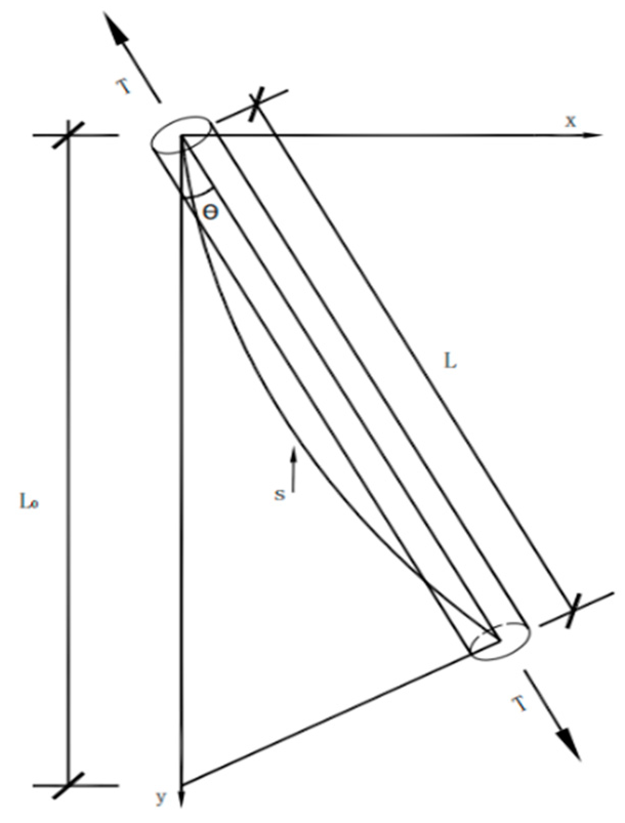
2. Derivation of Theoretical Formulae for Flexible Hanger
- (1)
- Articulated at both ends
- (2)
- Articulated at one end and fixed at the other
- (3)
- Fixed at both extremities
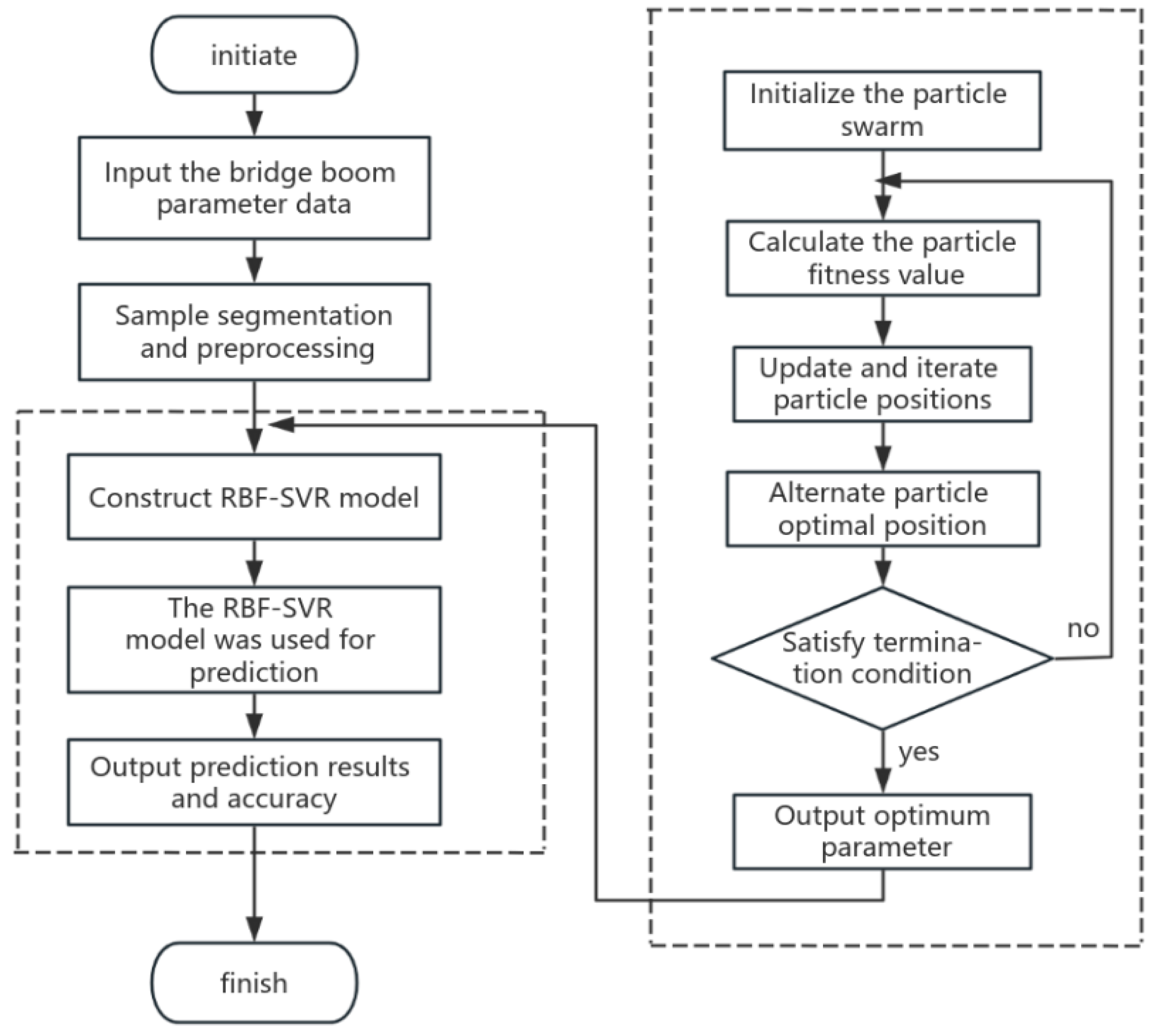
3. QPSO-RBF-SVM Model
3.1. RBF-SVM Modeling
3.2. QPSO Algorithm
3.3. Model Construction Steps
4. Modeling and Prediction Results
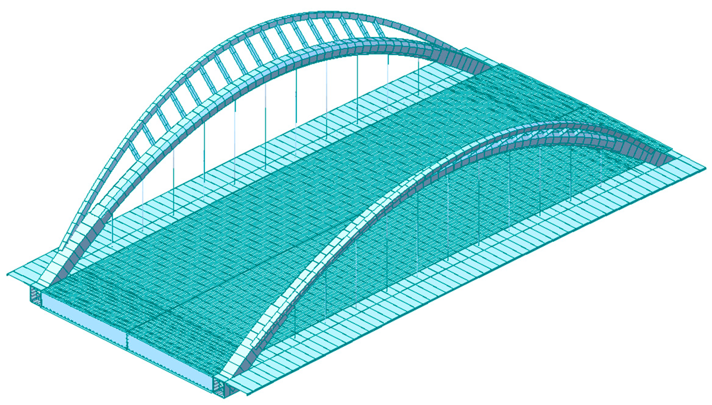
4.1. Project Overview
4.2. Data Collection
4.3. Data Processing and Model Building
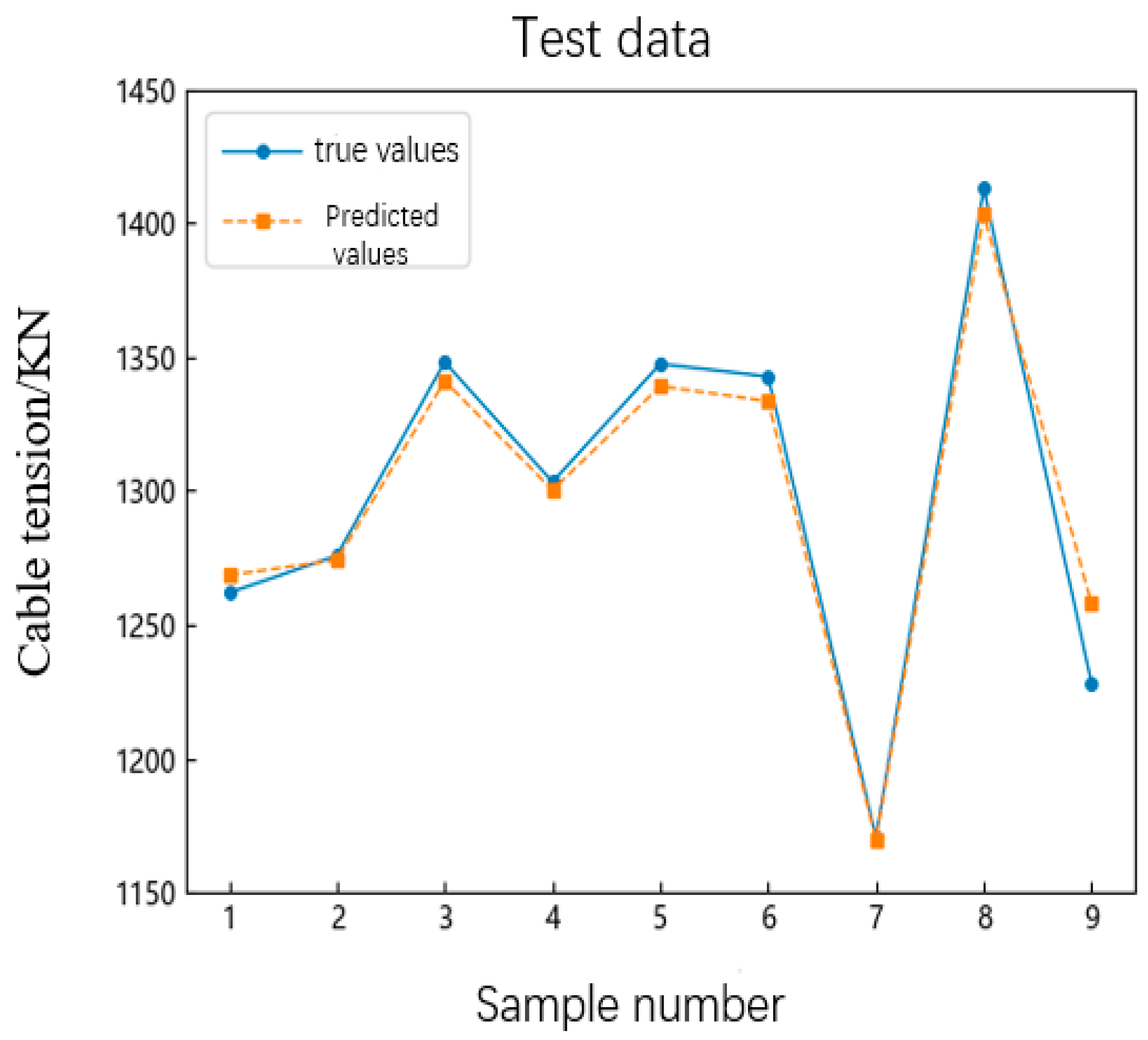
4.4. Prediction Results of Cable Force
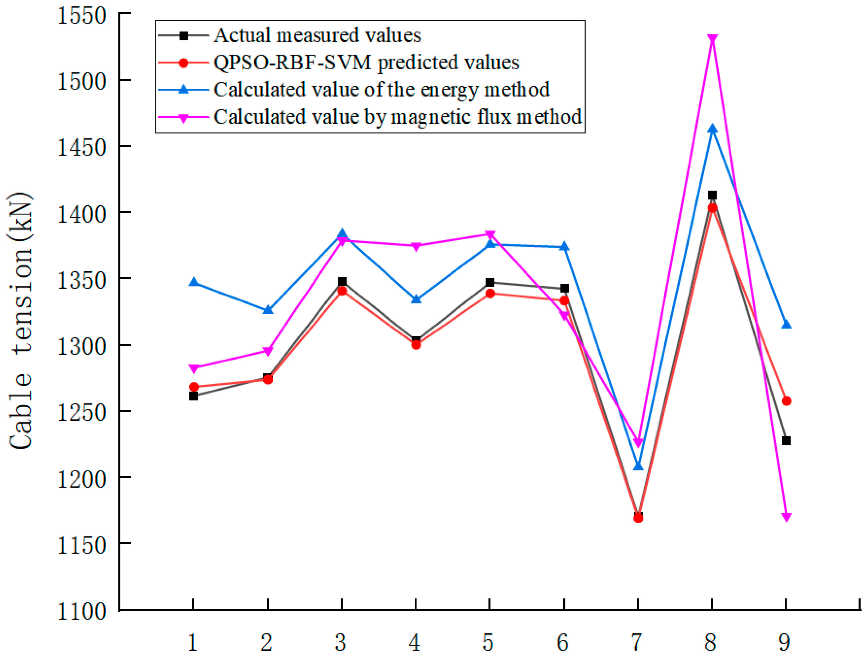
5. Comparative Analysis
5.1. Comparison with Formula
5.2. Comparison with Other Machine Learning Algorithms
6. Conclusions
Author Contributions
Funding
Institutional Review Board Statement
Informed Consent Statement
Data Availability Statement
Acknowledgments
Conflicts of Interest
References
- Liu, Z. Overview of Cable Force Testing Methods for Cable-Stayed Bridges. Railw. Constr. 2007, 4, 18–20. [Google Scholar]
- Zui, H.; Shinke, T.; Namita, Y. Practical formulas for estimation of cable tension by vibration method. J. Struct. Eng. ASCE 1996, 122, 665. [Google Scholar] [CrossRef]
- Ren, W.; Chen, G. Practical formulas for calculating cable tension from fundamental frequency. J. Civ. Eng. 2005, 11, 26–31. [Google Scholar]
- Liu, W.; Ying, H.; Liu, C. Precise solution for cable force considering stiffness and boundary conditions. J. Vib. Shock 2003, 22, 14–16+27+108. [Google Scholar]
- Chen, H.; Dong, J. Practical formulas for measuring cable tension of through and half-through arch bridges using the vibration method. China J. Highw. Transp. 2007, 3, 66–70. [Google Scholar]
- Yuan, P.; Xie, X.; Shen, Y. Testing methods and applications of hanger tension for arch bridges considering the impact of dampers. J. Zhejiang Univ. (Eng. Sci.) 2012, 46, 1592–1598. [Google Scholar]
- Fu, C.; Gao, Z.; Yan, P.; Tang, C.; Tang, B. Calculation method for reasonable completed bridge cable forces of concrete cable-stayed bridges based on the elastic support continuous beam method. Bridge Constr. 2022, 52, 124–130. [Google Scholar]
- Wang, X.; Deng, B.; Yang, M. Optimization study of hanger tension for high-speed railway tied arch bridges considering construction stages. J. Railw. Sci. Eng. 2020, 17, 808–814. [Google Scholar]
- Xiao, J.; Dai, Y.; Zhang, Y. Tension cable force identification method based on bending waves in substructures. J. Civ. Environ. Eng. 2020, 42, 135–143, (In Chinese and English). [Google Scholar]
- Ereiz, S.; Duvnjak, I.; Pajan, J.; Bartolac, M.; Damjanović, D. Determination of cable tension force in pedestrian suspension bridge short hangers based on finite element model updating. J. Phys. Conf. Ser. 2024, 2647, 122013. [Google Scholar] [CrossRef]
- Spasojević Šurdilović, M.; Živković, S.; Turnić, D. Algorithms for Computer-Based Calculation of Individual Strand Tensioning in the Stay Cables of Cable-Stayed Bridges. Appl. Sci. 2024, 14, 5410. [Google Scholar] [CrossRef]
- Xi, H.; Kaijian, L. Structural Deterioration Knowledge Ontology towards Physics-Informed Machine Learning for Enhanced Bridge Deterioration Prediction. J. Comput. Civ. Eng. 2023, 37, 04022051. [Google Scholar]
- Hussaini, J.; Bismark, A. Bridge Maintenance Planning Framework Using Machine Learning, Multi-Criteria Decision Analysis and Evolutionary Optimization Models. Autom. Constr. 2022, 143, 104585. [Google Scholar]
- Tian, X.; Jian, Y.; Long, C. Automated semantic segmentation of bridge point cloud based on local descriptor and machine learning. Autom. Constr. 2022, 133, 103992. [Google Scholar]
- Li, R.; Li, X.; Zheng, X.; Zhou, Y. Application of particle swarm algorithm in frequency-based hanger cable force identification. J. Vib. Shock 2018, 37, 196–201. [Google Scholar]
- Xie, W.; Zhou, X.; Qin, D.; Lu, C.; Tang, R. Prediction of construction cable forces of CFST arch bridge based on DNN. Structures 2024, 61, 106012. [Google Scholar] [CrossRef]
- Jianwei, B.; Peijun, C.; Hui, Z.; Sun, S.; Zhang, B.; Wang, Y.; Wang, L. Analysis of SF6 contact based on QPSO-SVR. Energy Rep. 2023, 9, 425–433. [Google Scholar]
- Ouyang, P.; Shen, Q.; Xie, X.; Zhu, W. Cable Force Identification and Finite Element Model Optimization of Cable-Stayed Bridges Based on Backpropagation Neural Networks. Transp. Res. Rec. 2023, 2677, 579–589. [Google Scholar] [CrossRef]
- Gai, T.; Yu, D.; Zeng, S.; Lin, J. An optimization neural network model for bridge cable force identification. Eng. Struct. 2023, 286, 116056. [Google Scholar] [CrossRef]
- Luo, K.; Kong, X.; Deng, L.; Wei, I.; Libo, M. Target-free measurement of cable forces based on computer vision and equivalent frequency difference. Eng. Struct. 2024, 314, 118390. [Google Scholar] [CrossRef]
- Clough, R.W.; Penzien, J.; Wang, G. Structural Dynamics; Science Press: Beijing, China, 1981. [Google Scholar]
- Hu, Z. Structural Vibration and Stability; People’s Communications Press: Beijing, China, 2008. [Google Scholar]
- Zhang, X. On statistical learning theory and support vector machines. Acta Autom. Sin. 2000, 1, 36–46. [Google Scholar]
- Zhang, L. Relationship between SVM with kernel function and three-layer feedforward neural networks. J. Comput. Res. Dev. 2002, 7, 696–700. [Google Scholar]
- Chen, P.; Yuan, L.; He, Y.; Luo, S. An improved SVM classifier based on double chains quantum genetic algorithm and its application in analogue circuit diagnosis. Neurocomputing 2016, 211, 202–211. [Google Scholar] [CrossRef]
- Hao, C.; Pei, M.; Qiang, S. New method for cable force testing of cable-stayed bridges—Magnetic flux method. Highway 2000, 11, 30–31. [Google Scholar]


| Spreader Bar Number | Length L (m) | Linear Density (kg/m) | Elastic Modulus E (kN/mm2) | Theoretical Cable (kN) |
|---|---|---|---|---|
| D1 | 7.149 | 42.20 | 195 | 1196 |
| D2 | 10.100 | 42.20 | 195 | 1276 |
| D3 | 12.385 | 42.20 | 195 | 1288 |
| D4 | 14.014 | 42.20 | 195 | 1287 |
| D5 | 14.990 | 42.20 | 195 | 1285 |
| D6 | 15.312 | 42.20 | 195 | 1285 |
| D7 | 14.981 | 42.20 | 195 | 1285 |
| D8 | 13.994 | 42.20 | 195 | 1287 |
| D9 | 12.348 | 42.20 | 195 | 1288 |
| D10 | 10.046 | 42.20 | 195 | 1276 |
| D11 | 7.102 | 42.20 | 195 | 1195 |
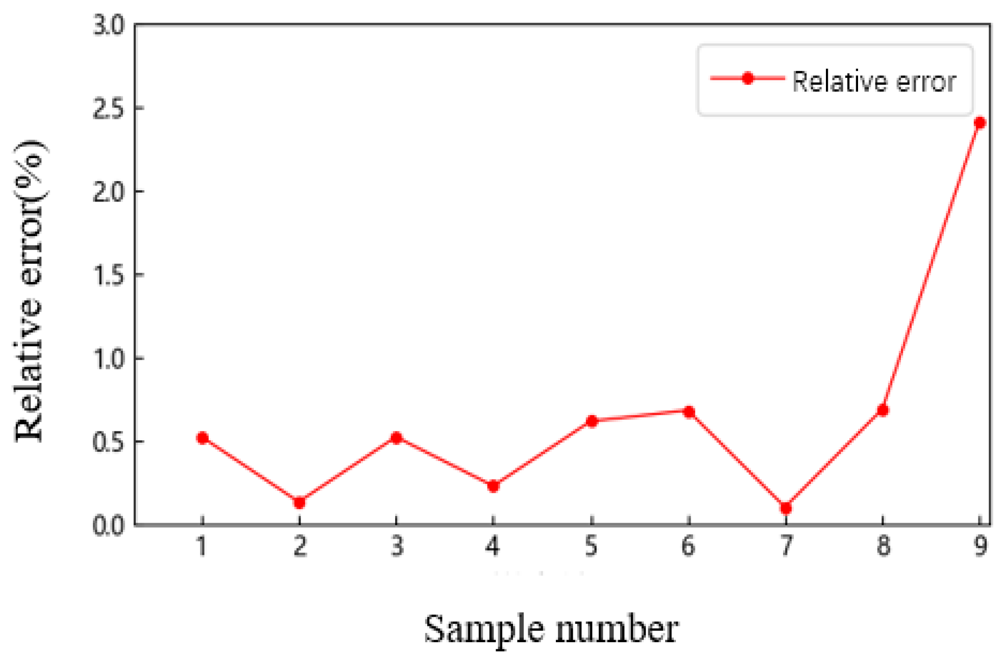
| Data Number | Actual Measured Value (kN) | Projected Value (kN) | Relative Error |
|---|---|---|---|
| 1 | 1261.89 | 1268.57 | 0.53% |
| 2 | 1275.78 | 1274.01 | −0.14% |
| 3 | 1348.07 | 1341.01 | −0.52% |
| 4 | 1303.29 | 1300.34 | −0.23% |
| 5 | 1347.37 | 1339.11 | −0.61% |
| 6 | 1342.61 | 1333.67 | −0.67% |
| 7 | 1170.76 | 1169.54 | −0.10% |
| 8 | 1412.81 | 1403.64 | −0.65% |
| 9 | 1228.15 | 1257.88 | 2.42% |
Disclaimer/Publisher’s Note: The statements, opinions and data contained in all publications are solely those of the individual author(s) and contributor(s) and not of MDPI and/or the editor(s). MDPI and/or the editor(s) disclaim responsibility for any injury to people or property resulting from any ideas, methods, instructions or products referred to in the content. |
© 2024 by the authors. Licensee MDPI, Basel, Switzerland. This article is an open access article distributed under the terms and conditions of the Creative Commons Attribution (CC BY) license (https://creativecommons.org/licenses/by/4.0/).
Share and Cite
Shi, H.; Shi, M.; Xu, W. Cable Tension of Long-Span Steel Box Tied Arch Bridges Based on Radial Basis Function-Support Vector Machine Optimized by Quantum-Behaved Particle Swarm Optimization. Appl. Sci. 2024, 14, 7163. https://doi.org/10.3390/app14167163
Shi H, Shi M, Xu W. Cable Tension of Long-Span Steel Box Tied Arch Bridges Based on Radial Basis Function-Support Vector Machine Optimized by Quantum-Behaved Particle Swarm Optimization. Applied Sciences. 2024; 14(16):7163. https://doi.org/10.3390/app14167163
Chicago/Turabian StyleShi, Hongcai, Menglin Shi, and Weisheng Xu. 2024. "Cable Tension of Long-Span Steel Box Tied Arch Bridges Based on Radial Basis Function-Support Vector Machine Optimized by Quantum-Behaved Particle Swarm Optimization" Applied Sciences 14, no. 16: 7163. https://doi.org/10.3390/app14167163
APA StyleShi, H., Shi, M., & Xu, W. (2024). Cable Tension of Long-Span Steel Box Tied Arch Bridges Based on Radial Basis Function-Support Vector Machine Optimized by Quantum-Behaved Particle Swarm Optimization. Applied Sciences, 14(16), 7163. https://doi.org/10.3390/app14167163