The Characteristics of the Spatial and Temporal Distribution of the Initial Compression Wave Induced by a 400 km/h High-Speed Train Entering a Tunnel

Abstract

The initial compression wave induced by a 400 km/h high-speed train entering a tunnel in two cases (offset running and center running) is investigated by overset mesh technology. The governing equations of the IDDES model for three-dimensional, unsteady, compressible flow are employed. The meshing strategy and numerical algorithm are validated by moving model test data. The spatial and temporal distribution characteristics of the initial compression wave and the one-dimensional planar wave characteristics are analyzed. The results show that the compression waves undergo three stages: from an irregular spherical shape near the train to an oblique shape, and finally to a one-dimensional planar wave. The initial compression wave captured at the measurement points at a distance of 5Di (Di represents the equivalent diameter of the tunnel) from the tunnel portal has been fully characterized by one-dimensional features, which can provide a boundary input for the propagation of the initial compression wave towards the tunnel exit. Compared to the offset running case, the initial compression wave amplitude and pressure gradient amplitude induced by central running are reduced by 3.66% and 6.87%, respectively.

1. Introduction

High-speed trains have greatly facilitated travel for people. With the development of technology, China, Japan, South Korea, Germany, and other countries are researching higher-speed high-speed trains. In 2021, China launched the “CR450 Technology and Innovation Project”, which will increase the train’s operating speed from 350 km/h to 400 km/h [1,2]. As train operating speeds increase, aerodynamics become a crucial factor, especially regarding the aerodynamic effects when trains pass through tunnels [3,4]. The initial compression wave is formed as the head car enters the tunnel and propagates through the tunnel at the speed of sound. When the compression wave reaches the tunnel exit, part of it is reflected back into the tunnel as an expansion wave, while another part radiates outside the tunnel as an impulse wave, known as a micro-pressure wave, as depicted in Figure 1 [5,6,7,8]. Micro-pressure waves are typically infrasound waves with frequencies below 20 Hz, which can cause doors and windows in nearby residential areas to vibrate [9,10]. More severe micro-pressure waves may take the form of audible noise, sometimes referred to as a sonic boom, causing noise pollution at the tunnel exit [11,12].

Previous studies have validated that the intensity of the micro-pressure wave is proportional to the maximum pressure gradient of the compression wave as it propagates to the tunnel exit [13]. The maximum pressure gradient of the initial compression wave in high-speed train tunnels is approximately proportional to the cube of the train’s speed [14]. The initial compression wave propagates as a one-dimensional plane wave toward the tunnel exit, and non-linear effects [15], friction [16,17], and tracks [18] affect the compression waveform and gradient. This causes the severity of the micro-pressure wave to vary depending on the length of the tunnel. It is evident that the hazards caused by micro-pressure waves induced by 400 km/h trains entering tunnels will be more severe [19,20]. This requires a comprehensive and integrated study of the generation mechanisms and mitigation methods. The research idea of our team is to use different methods to solve different regions according to the generation process of micro-pressure waves. Specifically, for the initial compression wave generation stage, a three-dimensional CFD numerical simulation method is used to explore the spatial and temporal evolution process of the initial compression wave. As the compression wave transitions from three-dimensional characteristics to a one-dimensional plane wave, the initial compression wave propagation process in tunnels of different lengths is simulated by a one-dimensional compressible unsteady non-isentropic flow model, and finally, the radiation of the micro-pressure wave near the exit is simulated by a three-dimensional CFD numerical simulation method. The focus of this study is on the initial compression wave generation stage, where we will obtain the one-dimensional waveform of the initial compression wave to provide boundary conditions for subsequent processes.

For the study of the initial compression wave, Hara [21] derived a first-order formula of the acoustic pressure term for the pressure rise of the compression wave generated. Howe [22] proposed an analysis method for the initial compression wave based on the non-linear acoustic theory using the formulation of the vortex sound theory. Over the years, this method has been the foundation for continuous and in-depth research on the initial compression wave caused by a train’s nose entering a tunnel. Different calculation methods for the initial compression wave have been proposed for various train nose shapes entering tunnels, as well as for various tunnel portals. These include unvented tunnel entrance hoods [23], flared portals [24], and vented hoods [25,26]. Bellenoue et al. [27] studied the three-dimensional effects of the flow field induced by a train entering a tunnel through scaled moving model experiments. The research clearly indicated that the three-dimensional effects of the compression wave diminish with increasing distance from the tunnel entrance. When the distance is greater than four times the tunnel diameter, the wavefront can be considered a plane wave. Wang et al. [28] investigated the three-dimensional characteristics of pressure waves in a 350 km/h train through a single-track tunnel. In recent years, researchers have conducted relevant optimization studies to reduce the pressure gradient of the initial compression wave. These include the optimization of the train nose shape [29,30,31] and the installation of tunnel hoods [32,33,34].

Currently, there is extensive research on the formation and mitigation measures of initial compression waves induced by high-speed trains traveling at speeds below 350 km/h through tunnels, while the spatial and temporal evolution characteristics of compression waves generated at higher speeds require further in-depth study. Given the above discussions, we will use a refined turbulence model to simulate the process of a high-speed train traveling at 400 km/h through a tunnel, exploring the spatial and temporal distribution characteristics of the initial compression wave and determining its one-dimensional waveform to provide boundary inputs for subsequent processes. The rest of this article is organized as follows: Section 2 details the geometric model, computational domain and boundary conditions, meshing strategy, numerical method, and verification. Section 3 discusses the generation mechanism, spatial and temporal distribution, and the one-dimensional waveform of the initial compression wave. Finally, concluding remarks are provided in Section 4.

2. Methodology

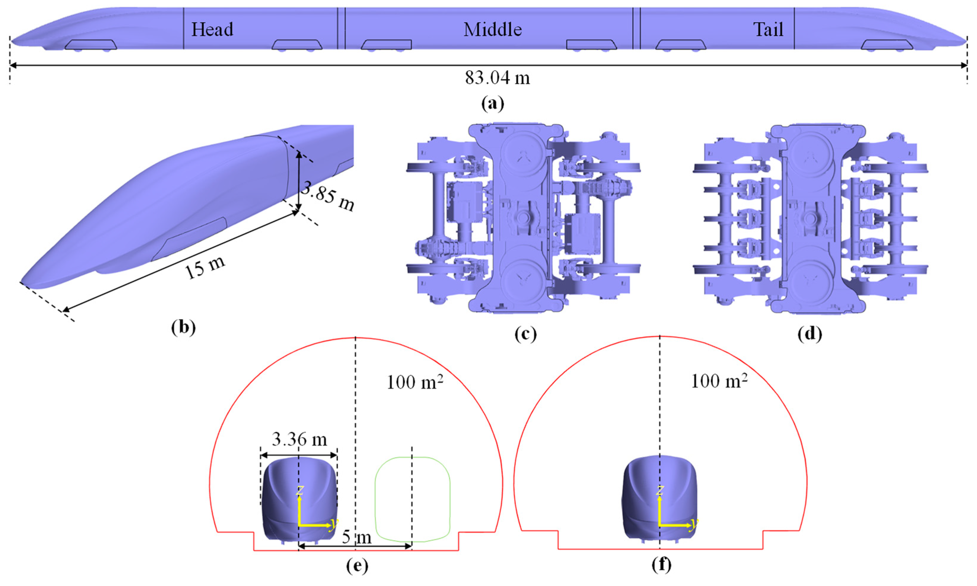
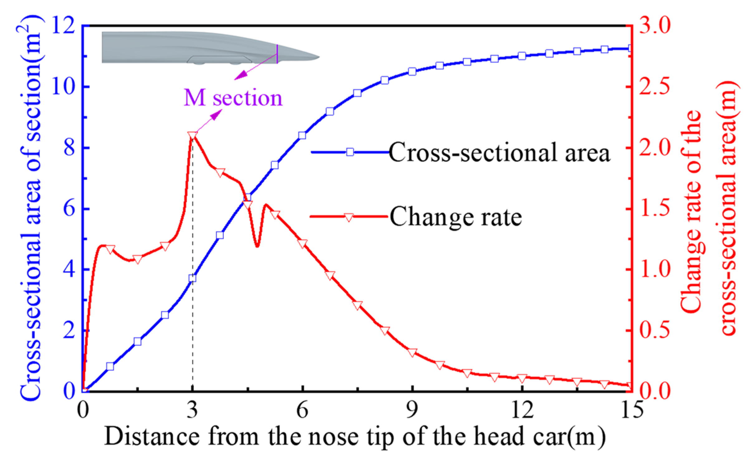
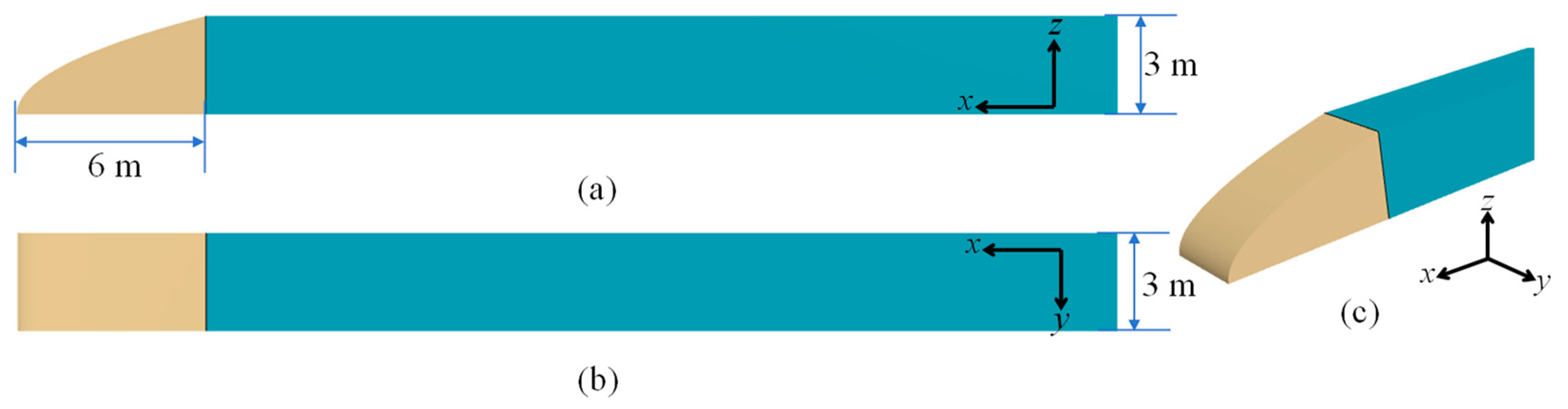
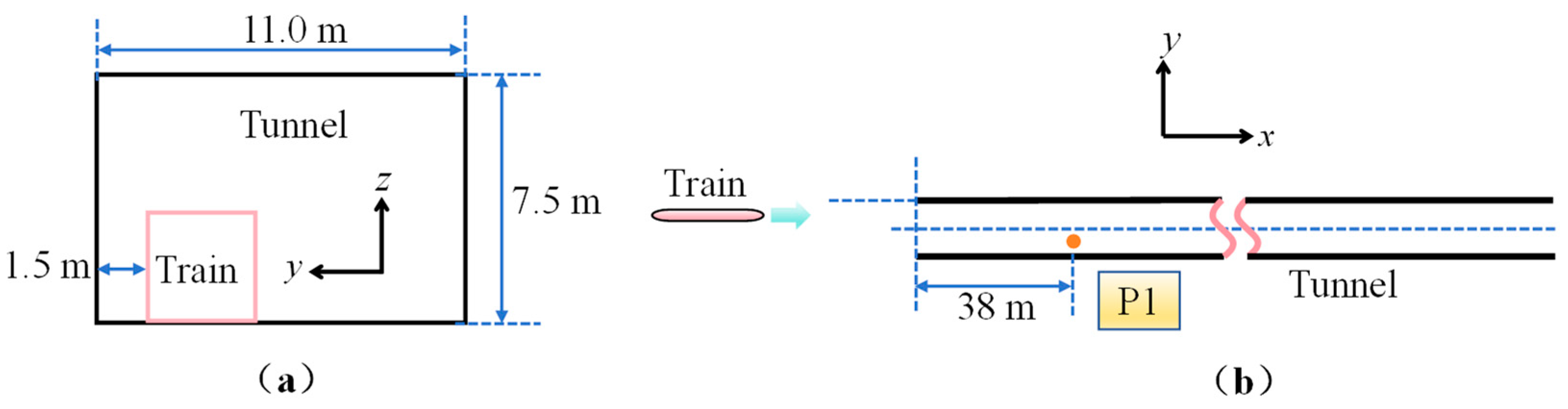
2.1. Geometric Model

Considering the minimal impact of train length on the pressure waves generated by the train entering the tunnel [35,36], a three-carriage of electric multiple units is used here, including the head car, the middle car, and the tail car, as illustrated in Figure 2. The train’s length (L_tr), width (W_tr), and height (H_tr) are 83.04 m, 3.36 m, and 3.85 m, respectively. The nose length of the train is 15 m. To accurately simulate the flow field around the high-speed train, the train model aims to faithfully reproduce the intricate original body structure, including the windshields, the powered bogies, the trailer bogies, and other structural components. To explore the correlation between the variation in the cross-sectional area of the train nose and the waveform of the initial compression wave, Figure 3 presents the distribution of the cross-sectional area and change rate of the streamlined train nose along the flow direction. The section where the maximum cross-sectional area change rate occurs is defined as the M section.

Considering the actual situation of railway tunnels in China, we selected a typical double-track tunnel with a cross-sectional area of 100 m², a line spacing of 5 m, and an equivalent diameter Di of 3.36 m [37,38,39]. To further study the spatial and temporal evolution characteristics of the initial compression wave with respect to the train’s running position, this research investigated two scenarios: one is offset running, which represents the actual operating case, and the other is center running, which serves as the control group. The origin of the coordinate system is set at the nose tip of the head car in two cases.

2.2. Computational Domain and Boundary Conditions

The overset mesh technology is employed here to reproduce the real motion of a train, which has been extensively used to examine trains traveling through tunnels or tubes [40,41,42]. The computational domain is divided into an overset region (moving region) close to the train and a background region (stationary region) including the tunnel and the area of the far field. The layout of the computational domain and the boundary conditions are illustrated in Figure 4. The schematic diagrams are not scaled to provide a better representation of the layout of the computational domain.

As this research primarily focuses on the initial compression wave characteristics induced by the train entering the tunnel, the computational domain does not include the far-field region of the tunnel exit [43,44], thus leading to a reduction in grid count and computation costs. To prevent pressure wave reflection, the far-field region and the tunnel exit are set with free-stream boundaries and non-reflective Riemann boundary conditions [45,46]. The dimensions of the computational domain are 300 m in the streamwise direction and 200 m in the vertical direction. At the initial moment, the high-speed train is positioned 280 m away from the far-field region on the left side. To avoid the numerical generation of compression waves, the train is gradually accelerated from a stationary state to 400 km/h using a fifth-order polynomial to describe the velocity profile [30], with an acceleration distance of 140 m. The expression for the velocity profile is as follows:

$$V_{tr}(t)={\displaystyle \frac{a}{20}}{t}^5-{\displaystyle \frac{a{t}_1}{8}}{t}^4+{\displaystyle \frac{a{t}_1^2}{12}}{t}^3,$$

(1)

where $a=120V_{tr}/t_1^5$, t₁ represents the acceleration time of the train and $V_{tr}$ denotes the speed at which the train enters the tunnel. This velocity expression ensures that the acceleration of the train is zero at both the beginning and the end of acceleration. At a distance of 100 m from the tunnel entrance, the train completes the acceleration process and then enters the tunnel at a constant speed of 400 km/h. The tunnel length is 500 m, and based on preliminary calculations and subsequent results, this length has been confirmed to ensure the generation of a complete initial compression wave. The far-field pressure is at a standard atmospheric pressure of 101,325 Pa, with a temperature of 288 K.

2.3. Meshing Strategy

The mesh configuration is consistent for center running and offset running cases. The mesh layout is presented here using the offset running case. The topology of the volume mesh is the prism layer mesh and trimmer mesh in STAR-CCM+ 18.02 software, which has been proven to be accurate in studying train aerodynamic issues [47,48]. As illustrated in Figure 5, according to the mesh strategy of Muld et al. [49] and considering the requirements for overset mesh, multi-level refinement blocks are applied around the train and wake region. The minimum grid size around the train is set to 0.05 m. To solve for the boundary layers on the train surface and the tunnel wall, 16 layers of prism layer mesh are applied to the train surface with a stretching ratio of 1.2, resulting in a total thickness of 118.12 mm. Similarly, the tunnel wall is stretched with 16 layers and a stretching ratio of 1.2, resulting in a total thickness of 78.7 mm. To reduce discretization errors, it is necessary to ensure that the grid cell sizes in the overlapping regions of the two sets of meshes remain identical. The total number of mesh cells in the computational model is 32.84 million, with 5.45 million cells in the background region and 27.39 million cells in the overset region.

2.4. Numerical Method

For spatial discretization, the control equations are discretized using the finite volume method. Considering computational resources, we choose to use a segregated flow solver to solve the discretized algebraic equation system. Additionally, we employ the semi-implicit method for pressure-linked equations (SIMPLE) to address the coupling between velocity and pressure in the control equations. For turbulence modeling, the Improved Delayed Detached Eddy Simulation (IDDES) method is used, specifically, the Shear Stress Transport (SST) k-ω model [50] for turbulence closure. Detached Eddy Simulation (DES) is a hybrid modeling approach that employs the Reynolds-Averaged Navier-Stokes (RANS) model to solve boundary layers and irrotational flow regions while using Large Eddy Simulation (LES) for other regions. IDDES is an improved form of the DES model that provides the DES model with Wall-Modeled LES (WMLES) capabilities, achieving a balance between computational accuracy and time to some extent. This method has been widely used in the study of aerodynamic characteristics of high-speed trains [51,52].

The convective flux terms are discretized using a second-order upwind/bounded central differencing hybrid method with a blending factor of 0.15, meaning 15% second-order upwind interpolation and 85% bounded central differencing. The temporal term is discretized using a second-order implicit scheme. The time step for the computational model is set to 4.4 × 10⁻⁴ s, ensuring that the maximum Courant number does not exceed 1.0 and meets the time step requirements for the overset mesh method. The maximum number of inner iterations per time step is 10. As the grid size increases, the convergence speed of traditional iterative solving algorithms such as Jacobi, Gauss–Seidel, and ILU significantly decreases, leading to increased computation time. To improve the robustness and convergence speed of the linear systems generated by the solver, the Algebraic Multigrid (AMG) method is used. The simulations were conducted on a supercomputer, utilizing 4 nodes. Each node was configured with 2 × X86 7285H processors, 256 GB of memory, and 32 cores. The total simulation time was approximately 32 h.

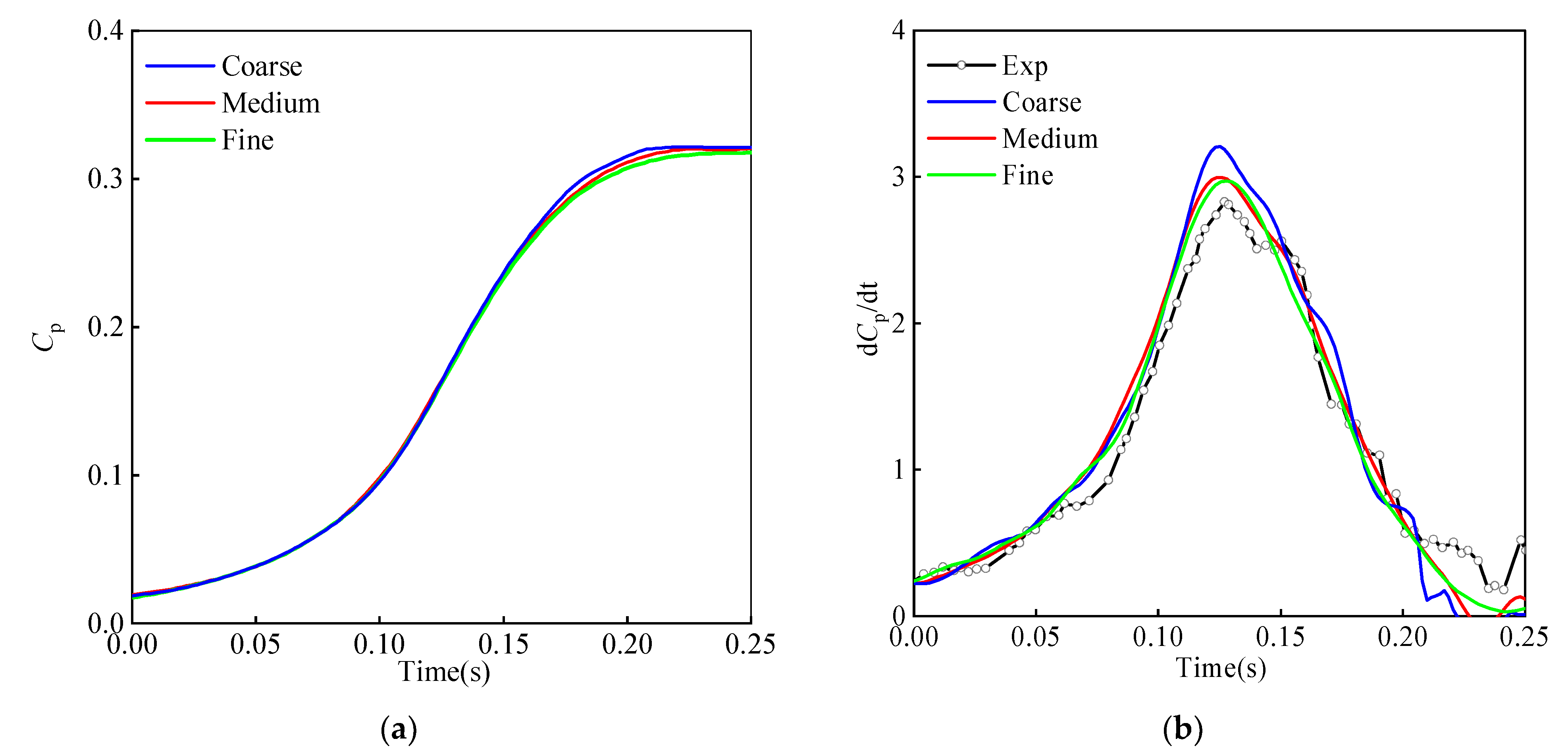
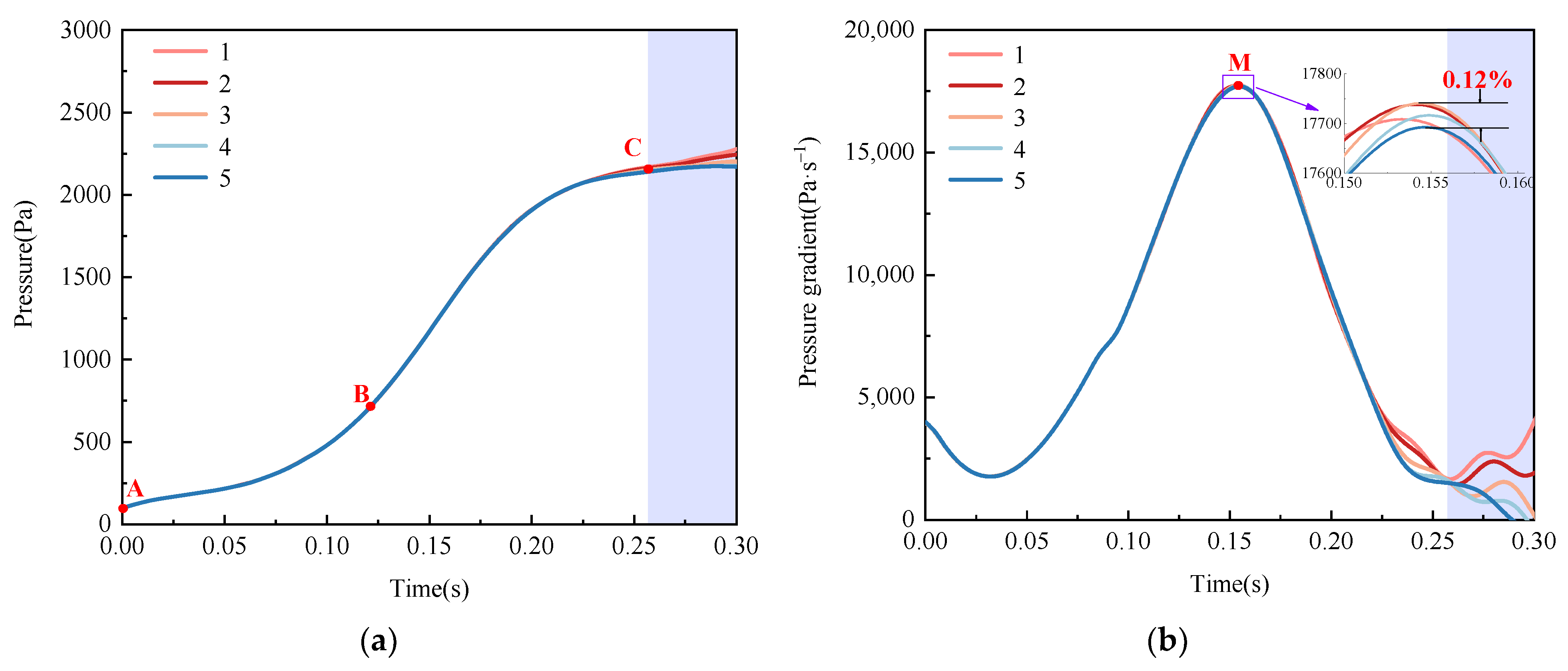
2.5. Mesh-Independent and Numerical Methods Validation

Here, the result of a 1:30 scaled moving model experiment [53] where the train with a parabolic wedge nose traveling through the tunnel at 360 km/h is chosen to verify the accuracy of the mesh strategy and numerical method. As presented in Figure 6, the nose is a parabolic wedge shape. In the full-scale model, the streamlined nose of the train is 6 m long, and the train’s width and height are both 3 m. Figure 7 illustrates the distribution of the tunnel/train model and the arrangement of measurement points. The tunnel model is a square-section tunnel with a width of 11 m and a height of 7.5 m. The distance between the train and the tunnel wall is 1.5 m. Measurement point P1 is placed 38 m from the tunnel entrance to capture the initial compression wave. The movement of the train inside the tunnel is achieved through overset mesh method, with numerical methods and grid strategies consistent with those described in Section 2.3 and Section 2.4.

To conduct a mesh independence study, three sets of meshes with consistent strategies but different sizes are developed. The coarse, medium, and fine meshes have 2.49, 3.96, and 6.90 million cells, respectively.

Table 1. The comparison of mesh resolutions and a maximum pressure coefficient gradient of P1.

Case	Coarse	Medium	Fine
Total of cells (million)	2.49	3.96	6.90
No. of prism layers	16	16	20
Minimum cell size (m)	0.06	0.05	0.04
Maximum pressure coefficient gradient	3.21	2.99	2.97
Relative error (%)	13.43	5.65	4.95

lists the key meshing parameters for the three sets of meshes. The size and layout of the medium-density mesh are consistent with those described in Section 2.3. Figure 8 compares the time histories of the pressure coefficient and pressure coefficient gradient at point P1 calculated by the three sets of meshes. It also compares the time history of the pressure coefficient gradient with the experimental results. The initial compression waveforms captured by the three sets show consistent trends, with differences in amplitude being less than 1.40%. In terms of the pressure coefficient gradient, the computational results from the three mesh sets are generally consistent with the experimental trends, and the time of obtaining the maximum pressure coefficient gradient is also relatively close. However, there are significant differences in the maximum pressure coefficient gradient values. Compared to the experimental results, the relative errors for the coarse, medium, and fine meshes are 13.43%, 5.65%, and 4.95%, respectively. In summary, considering both computational resources and accuracy, the medium mesh strategy is chosen for the study of the 400 km/h train passing through the tunnel scenario.

3. Results and Discussion

This section begins by analyzing the generation mechanism of the initial compression wave, one-dimensional and three-dimensional characteristics of the initial compression wave, and the formation position of the one-dimensional waveform of the entire initial compression wave in the case of offset operation. Subsequently, a comparative study is conducted to examine the impact of the train’s running position on the characteristics of the initial compression wave.

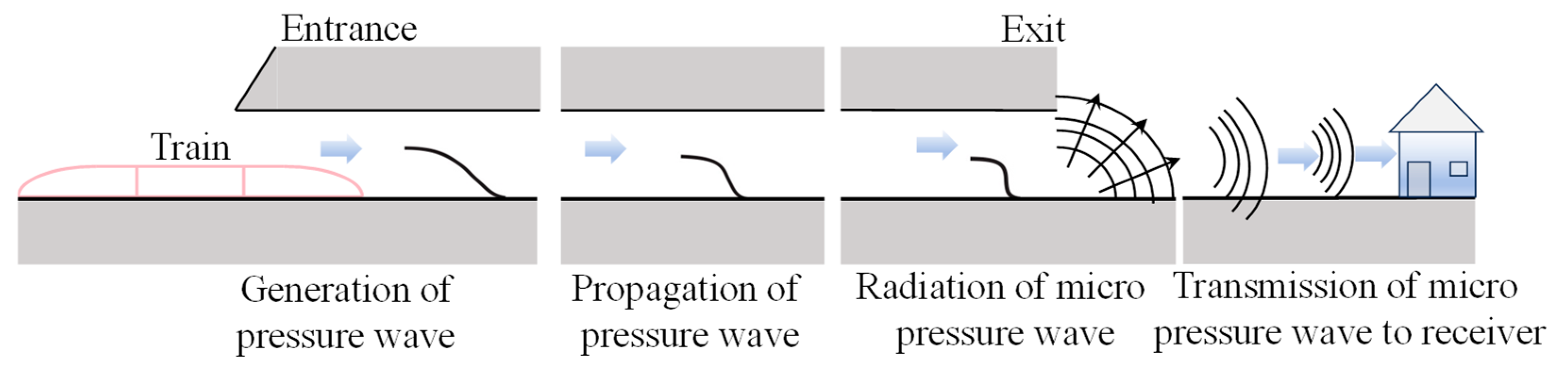
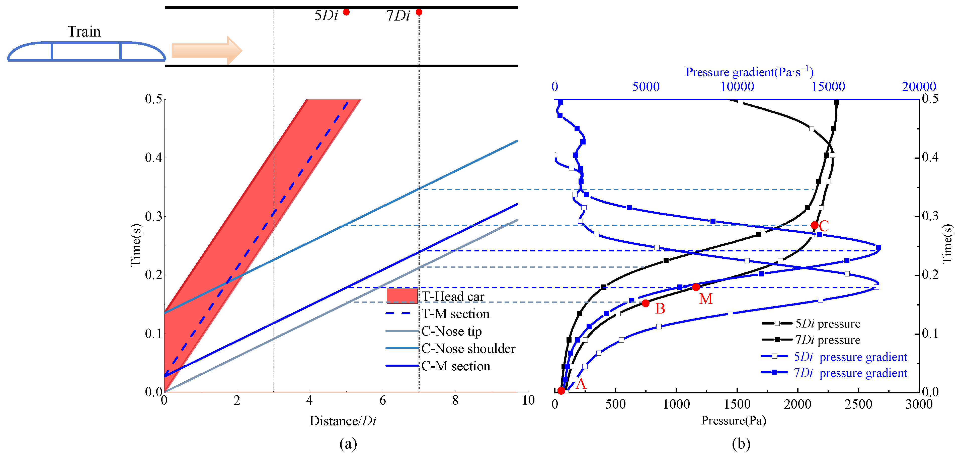
3.1. The Generation Mechanism of the Initial Compression Wave

The complex pressure waves are generated as a high-speed train passes through a tunnel. Figure 9 depicts a schematic of pressure fluctuations at a measurement point within the tunnel. There are four primary processes in which the pressure changes at a measurement point within the tunnel. When the train’s streamlined nose enters the tunnel, there is a rapid initial rise in pressure (Δp_N), commonly referred to as the initial compression wave. This is also the focus of this research. The second pressure rise (Δp_fr) is caused by the friction produced by the body part of the train entering the tunnel. The third process involves pressure decrease (Δp_T) caused by the expansion wave generated as the tail car enters the tunnel. When the head car passes through the measuring location, the pressure drops significantly (Δp_Hp) [4].

To illustrate the formation mechanism and process of the initial compression wave, Figure 10 depicts the time history of the initial compression wave and pressure gradient at roof measurement points located 5Di and 7Di away from the tunnel entrance. The moment when the train’s nose reaches the tunnel entrance is defined as 0 s.

As shown in Figure 10, before the train enters the tunnel, the pressure at the measurement points inside the tunnel begins to rise. This is because the pressure disturbances generated by the train’s movement in the open air propagate into the tunnel, causing the pressure to increase. The pressure rises due to the disturbances from the open air at the measurement points located at 5Di and 7Di are 708 Pa and 705 Pa, respectively. As the train’s nose enters the tunnel, a sequence of compression waves is generated due to the variation in the annular cross-section of the train and the tunnel. The compression waves generated from the train’s nose and shoulder propagate to the measurement points, denoted as points B and C, respectively. As a result, the AB segment of the pressure-time history curve is attributed to disturbances from the open air, while the BC segment is attributed to the train’s nose entering the tunnel.

Simultaneously, the distribution of the pressure gradient of the initial compression wave is closely related to the distribution of the nose-shaped cross-sectional area along the length of the train’s nose. As the part of the streamlined nose with the maximum cross-sectional area change rate (denoted as the M section) enters the tunnel, the resulting compression wave causes the largest pressure gradient at the measurement point. Therefore, to mitigate the intensity of the micro-pressure wave, it is advisable to minimize abrupt changes in the cross-sectional area of the head shape.

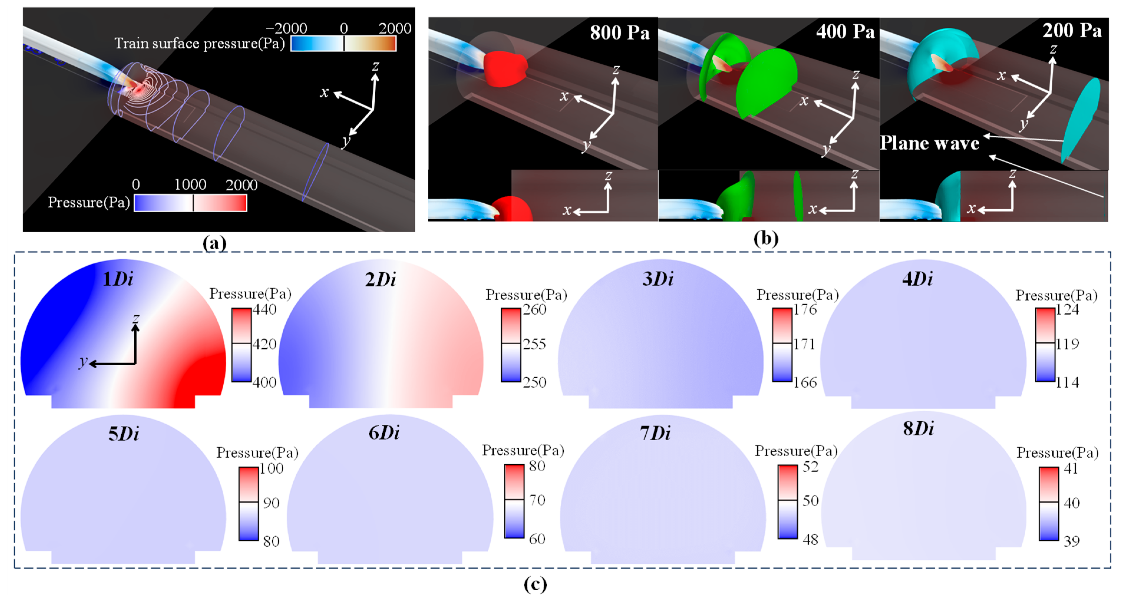
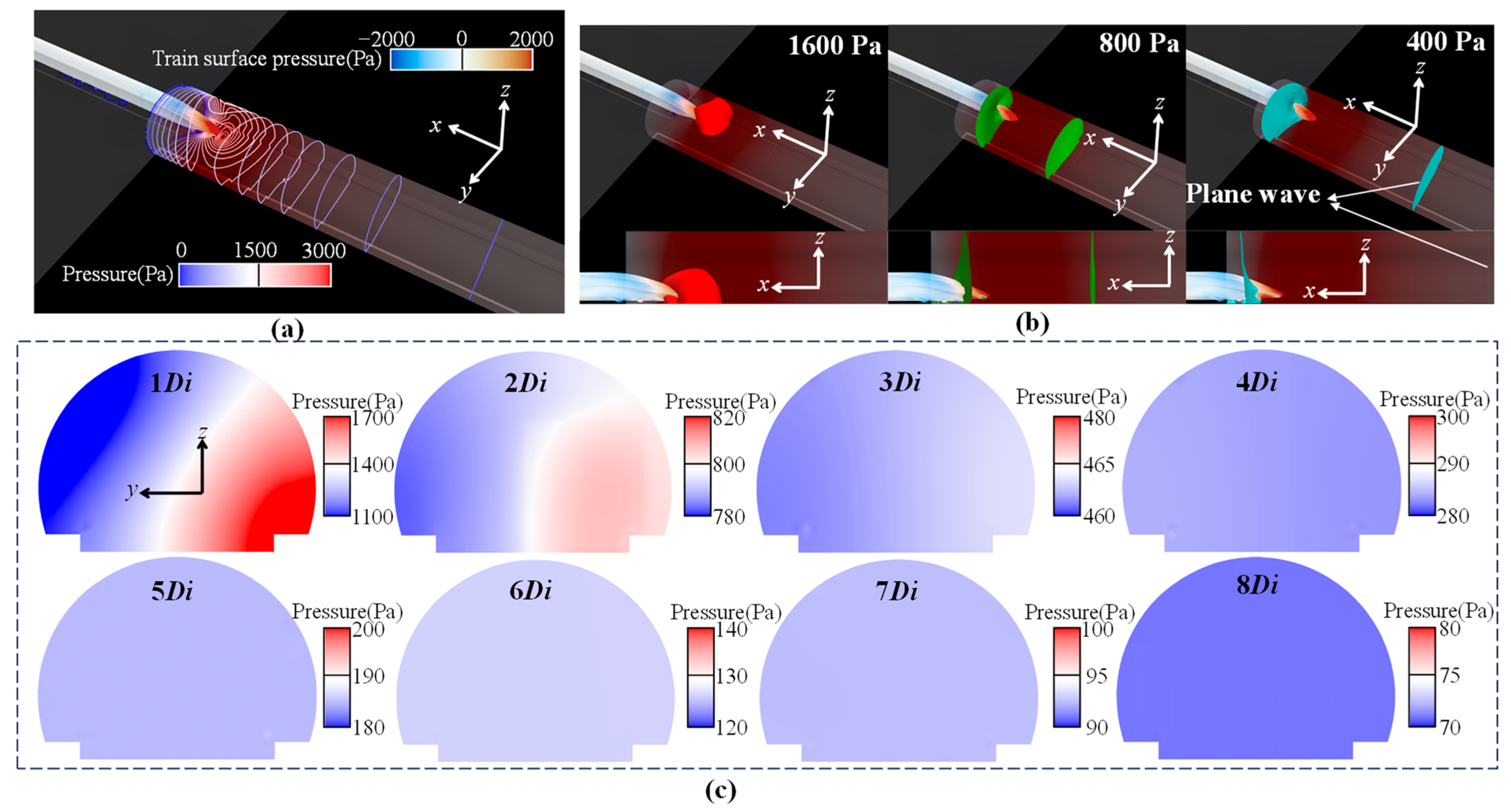
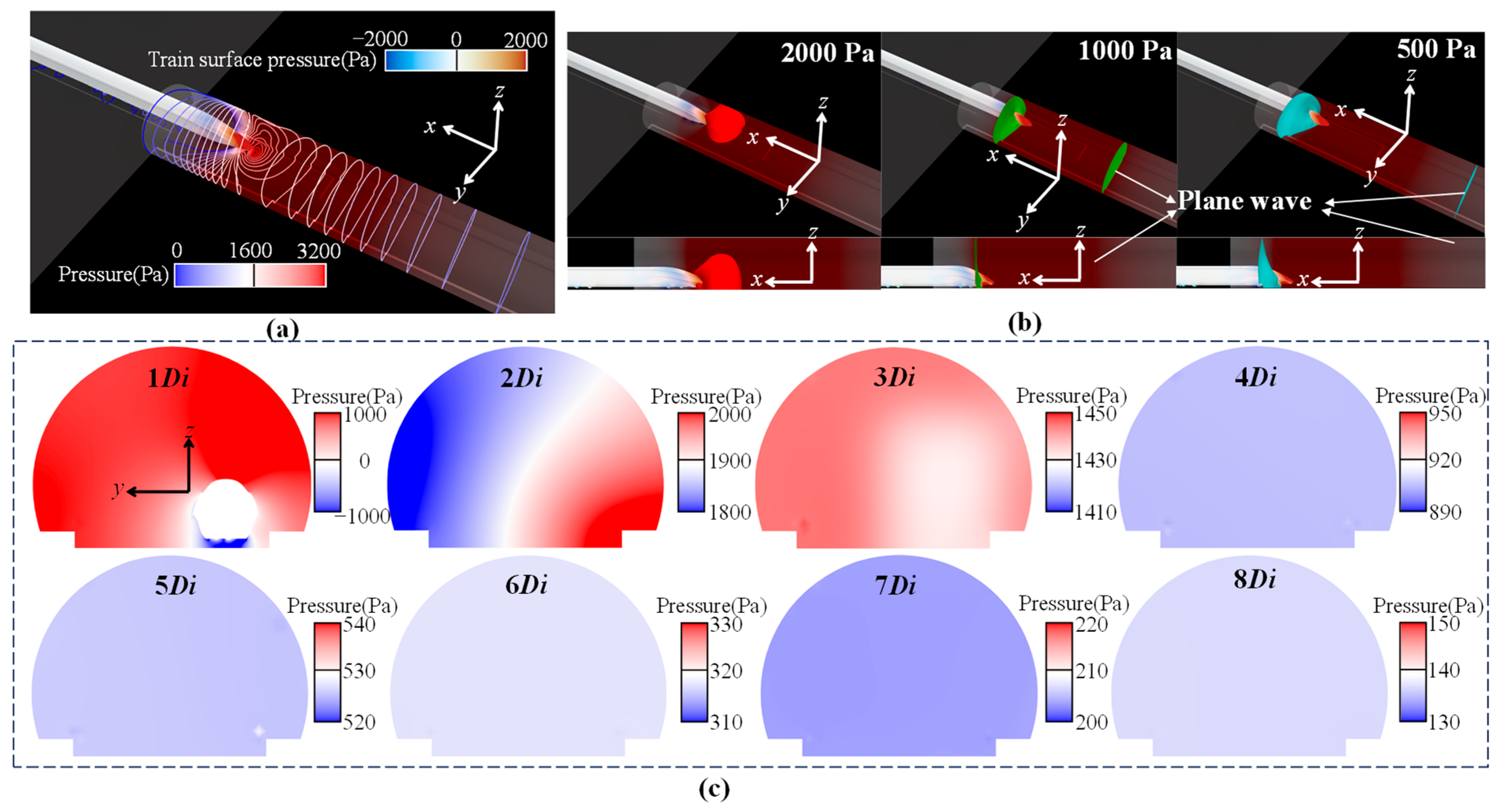
3.2. The One-Dimensional and Three-Dimensional Characteristics of the Initial Compression Wave

As shown in Figure 11, at 0 s, the nose tip of the head car just approaches the tunnel entrance, and compression waves generated by the train’s movement in the open air have propagated into the tunnel, causing pressure changes. This is consistent with the behavior shown in the pressure–time history curves of the measurement points in Figure 10. The pressure distribution near the train’s head inside the tunnel exhibits distinct three-dimensional characteristics. The tunnel wall closer to the train has higher pressure compared to the side away from the train. As depicted in Figure 11b, high-pressure regions close to the head car have been detected using the pressure iso-surface at 800 Pa. Due to limitations imposed by the ground, the tunnel walls, and the curvature of the train’s head, this iso-surface exhibits an irregular spherical shape. By employing lower pressures, the pressure iso-surface divides into two parts: one part represents the pressure distribution near the train body, and the other part represents the compression wave in front of the train. It is noteworthy that the pressure iso-surface at 400 Pa capturing the compression wave in front of the train is not perpendicular to the flow direction, presenting an oblique shape. This indicates that it is still influenced by the three-dimensional effect of the head car. However, the pressure iso-surface at 200 Pa capturing the compression wave in front of the train is located further away from the train, and the compression wave surface becomes perpendicular to the flow direction, evolving into a one-dimensional plane wave. To quantitatively analyze the transition of the three-dimensional effect of compression waves to one-dimensional plane waves, the pressure distributions at eight tunnel cross-sections are displayed, ranging from 1Di to 8Di away from the tunnel entrance, as shown in Figure 11c. At the 1Di cross-section, it is evident that the pressure inside the tunnel near the train side is significantly greater than the pressure on the side away from the train, and the maximum pressure is located at the bottom of the tunnel on the right side (near the train). This is mainly due to the compression of air in front of the train caused by its motion, which leads to the air dispersing outward. However, the ground and the tunnel wall near the train restrict the downward and outward flow, causing air accumulation and an increase in pressure. As the cross-sections move farther away from the tunnel entrance, the differences between high-pressure and low-pressure decreases. In the 3Di cross-section, the pressure distribution becomes more even, exhibiting one-dimensional characteristics.

As shown in Figure 12, at 0.0675 s, the train’s half-nose length enters the tunnel, causing a significant increase in spatial pressure in front of the train. Meanwhile, the pressure difference in the tunnel cross-section near the train increases. In the 1Di cross-section, the pressure difference exceeds 600 Pa. Similar to the scenario at 0 s, the higher-pressure (1600 Pa) iso-surface represents the high-pressure area near the train’s nose, while the lower-pressure iso-surfaces (800 and 400 Pa) represent the pressure distribution around the train and the compression wave in front of the train. In the 4Di cross-section, the pressure distribution becomes more even, exhibiting one-dimensional characteristics. As shown in Figure 13, at 0.135 s, the entire nose length of the train enters the tunnel, and the spatial pressure in front of the train further increases, approaching saturation. The initial compression wave has fully formed, but it will take some time for the subsequent compression waves to propagate to the measurement point. As depicted in Figure 13b, the initial compression waves captured by the pressure iso-surfaces at 500 and 1000 Pa are both plane waves. In the 4Di cross-section, the pressure distribution becomes more even, exhibiting one-dimensional characteristics.

Based on the above analysis, the compression waves exhibit three-dimensional characteristics near the train, while one-dimensional plane waves always appear at a certain distance in front of the train. To quantify the transition of the compression wave from three-dimensional to one-dimensional characteristics, Figure 14 illustrates the distribution of maximum and minimum pressures inside the tunnel at different times and provides the change ratio of pressure difference to identify the critical transition location. The formula for calculating the pressure difference ratio η is as follows:

η = |(p_max − p_min)/p_max|,

(2)

where p_max and p_min represent the maximum pressure and minimum pressure, respectively.

Here, we consider that if the pressure difference ratio η of a section is less than 1%, then the pressure distribution on that section is even. At 0 s and 0.0675 s, the train has not yet reached the 1Di section. From the 1Di to 8Di sections, both the pressure amplitude and the pressure differential ratio gradually decrease, becoming one-dimensional characteristics at the 3Di and 4Di sections, respectively. At 0.135 s, the 1Di section is located at the train body, exhibiting significant three-dimensional characteristics. The maximum negative pressure is detected at the bottom of the train, with a pressure differential ratio reaching 95.39%. The 2Di section, located in front of the train, shows a substantial increase in both maximum and minimum pressures, with a pressure differential ratio of 11.06%. Following the 4Di section, the pressure differential ratio decreases to below 1%. At 0.2025 s and 0.27 s, one-dimensional plane waves form at positions 4Di and 5Di, respectively.

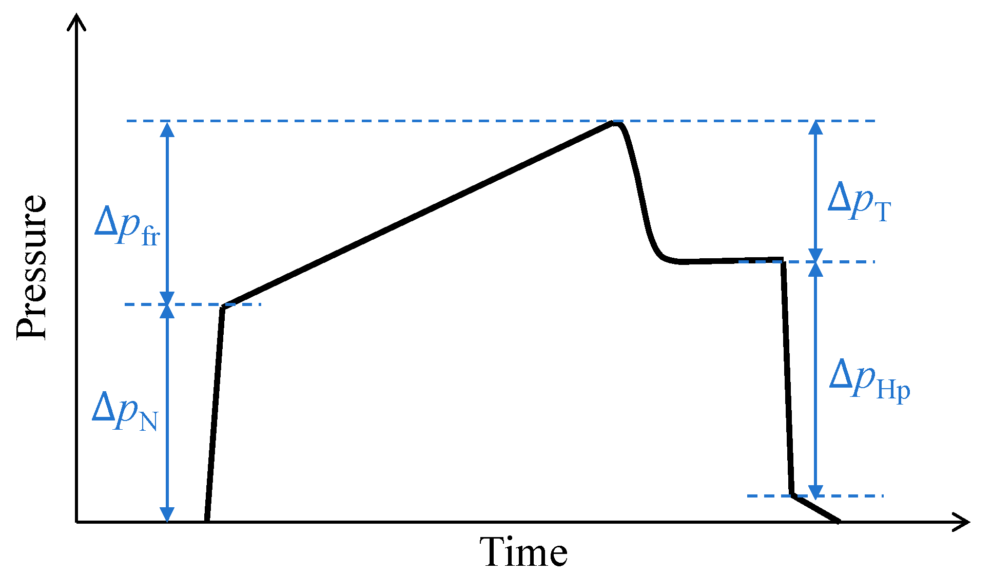
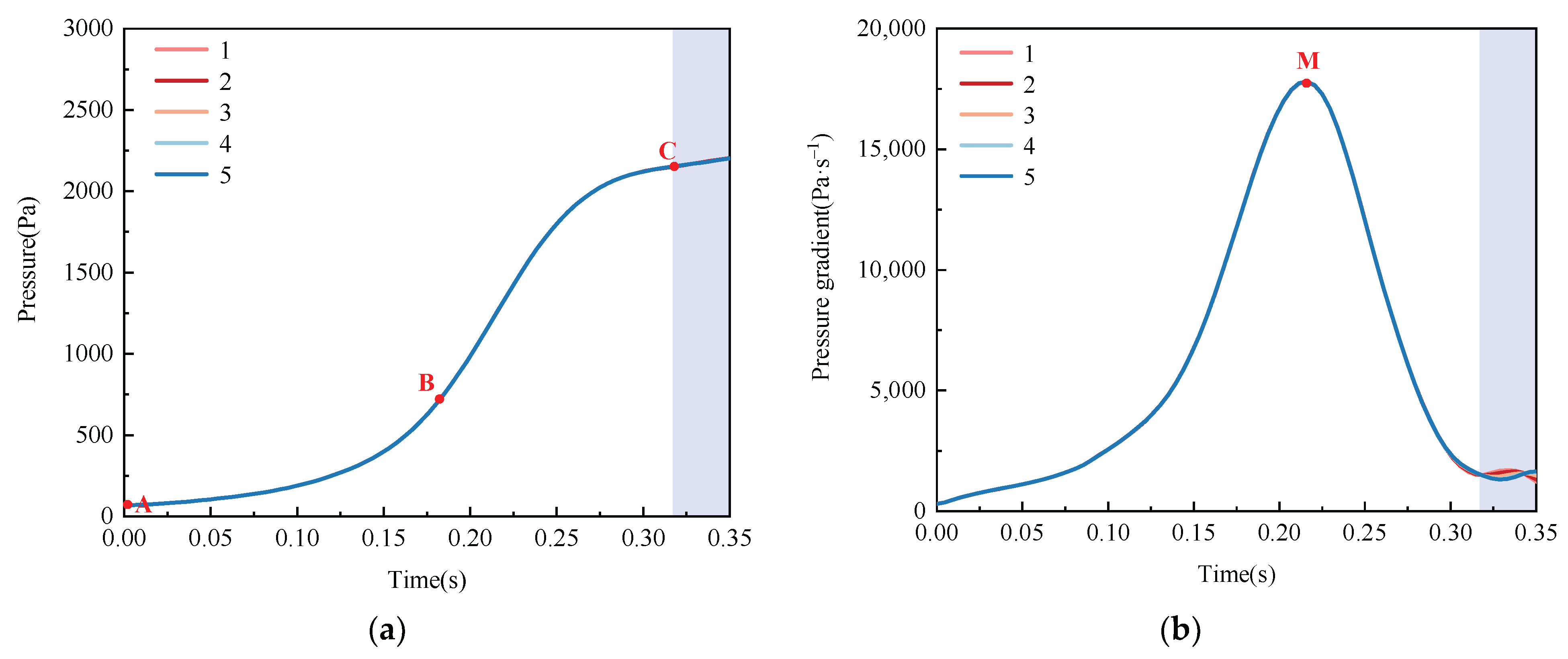
3.3. The Identification of One-Dimensional Waveform of the Entire Initial Compression Wave

The one-dimensional and three-dimensional characteristics of the initial compression wave have been elucidated in Section 3.2. To provide boundary conditions for the propagation of the initial compression wave, the initial compression wave at measurement points needs to meet two conditions: firstly, it must exhibit the entire waveform of the initial compression wave, and secondly, it must have already evolved into a one-dimensional feature. Therefore, this section will determine the waveform that provides boundary conditions for the propagation of the initial compression wave.

As shown in Figure 15, measurement points are located at sections 3Di~6Di from the tunnel entrance, with five measurement points arranged at each section. Two measurement points are set at a height of 1.8 m above the ground, located on the left and right tunnel walls, labeled as points 1 and 5. Points 1 and 5 form point T with the centerline of the tunnel. Taking point T as the origin, draw rays at a 45° angle to the centerline of the tunnel. The intersection points of these rays with the tunnel wall are designated as points 2 and 4. The point at the top of the tunnel is designated as point 3. Previous studies have shown that the intensity of micro-pressure waves is closely related to the pressure gradient of the initial compression wave. Given this, Figure 16, Figure 17, Figure 18 and Figure 19 compare the waveforms and the pressure gradients of the initial compression waves at five measurement points from 3Di to 6Di cross-sections.

According to Figure 16, the waveforms of initial compression waves captured by the 5 points on the 3Di cross-section exhibit consistency in the AB segment, but there are significant differences in the BC segment. This indicates that the disturbances generated by the train during open-air operation have already transitioned into one-dimensional characteristics at the 3Di cross-section, whereas the pressure disturbances generated when the train enters the tunnel still exhibit three-dimensional characteristics at the 3Di cross-section. Among them, point 1 has the highest pressure (i.e., the maximum amplitude of the initial compression wave) at C, followed by point 2, and the lowest is at point 5. This indicates that under three-dimensional effects, the amplitude of the compression wave is closely related to the distance of the measuring point from the train. Point 1 has a pressure amplitude 10.21% greater than that of point 5. Additionally, the amplitude of pressure gradients is also closely related to the distance of the measurement point from the train. Compared to point 1, the amplitude of pressure gradients at point 5 has decreased by 2.31%.

As shown in Figure 17, the waveforms of initial compression waves at various points in the 4Di section are similar to those in the 3Di section. The BC segment is still affected by the three-dimensional effect of the train’s nose, but compared to the 3Di section, this effect is weakened. Although the maximum pressure gradient differences of the initial compression waves at the five measurement points are negligible (0.21%), there is a considerable variance in pressure gradient near point C. As illustrated in Figure 18 and Figure 19, the waveforms of the initial compression wave captured by five measurement points at the 5Di and 6Di cross-sections are consistent, exhibiting one-dimensional characteristics. Comparing the waveform and pressure gradient distribution of the initial compression wave between the 5Di and 6Di cross-sections, both the pressure amplitude and the maximum pressure gradient amplitude are less than 1%, indicating that the initial compression wave captured at the 5Di cross-section is complete. Based on the above analysis, the initial compression wave captured by the cross-sections after 5Di has been fully and exhibits one-dimensional characteristics, which can provide boundary input for the propagation process of the initial compressed wave.

3.4. The Influence of Train Running Position on the Initial Compression Wave

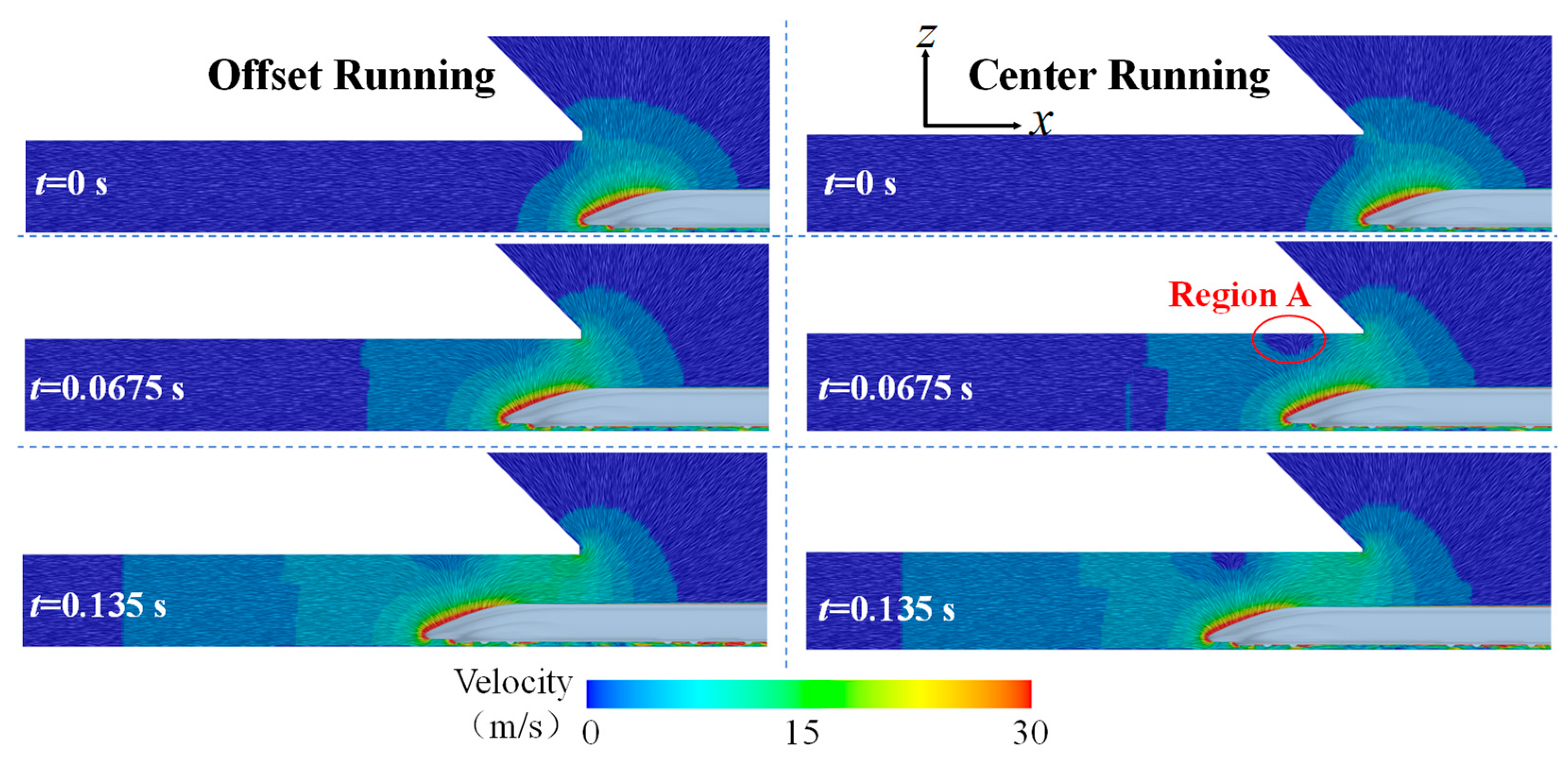
3.4.1. Comparison of the Transition Process of the Initial Compression Wave from Three-Dimensional Wave to One-Dimensional Wave

Figure 20 and Figure 21, respectively, show the velocity vector distribution at the nose height horizontal cross-section (z = 0 m) and the train longitudinal center cross-section (y = 0 m) during the process of the head car entering the tunnel. The line integral convolution (LIC) display method is used, with coloring according to the velocity magnitude. At t = 0 s, when the train nose enters the tunnel, a strong forward-pushing effect forms in front of the head car. The flow, constrained by the tunnel space, propagates into the tunnel, creating a tunnel compression wave. At this moment, the lateral and rearward displacement effects are relatively weak, resulting in weaker pressure and velocity disturbances that exhibit the characteristics of an expansion wave. As it propagates outside the tunnel, it generates a negative pressure pulse, forming the tunnel entry wave [54]. Not surprisingly, from a spanwise perspective, there are significant differences between offset running and center running cases. The disturbances generated by the offset running are not perpendicular to the flow direction, while the center running maintains a symmetric disturbance pattern. From a vertical perspective, the disturbances generated by both running modes are similar, exhibiting three-dimensional characteristics. This is attributed to the constraints imposed by the wall surfaces and the ground effect.

At t = 0.0675 s, the curved portion of the train’s nose begins to enter the tunnel. The tunnel walls severely restrict the diffusion of the compressed air. Most of the air compressed by the train continues to move inside the tunnel along the direction of the train’s travel, while some of the compressed air escapes through the annular space out of the tunnel. In the spanwise direction, the uneven distribution of the flow field near the train running in an offset case leads to the pressure wave exhibiting three-dimensional characteristics. However, the pressure disturbance farther away from the train already exhibits one-dimensional characteristics. The disturbances generated in the vertical direction by the two operating conditions are quite similar, except for a local stagnation area that appears at the top of the tunnel in the centerline running condition (Region A in Figure 21). This local stagnant zone is caused by the airflow flowing towards both sides of the tunnel. At t = 0.135 s, the streamlined nose of the train is fully inside the tunnel, and the compression wave generated by the nose reaches saturation. The differences in flow disturbances generated by the two operating cases are similar to those at t = 0.0675 s.

To compare the influence of the train running position on the three-dimensional characteristics of the compression wave, the pressure iso-surfaces at t = 0.2025 s are used for visualization. As depicted in Figure 22, high-pressure regions close to the head car have been detected using the pressure iso-surface at 2400 Pa. By comparison, the high-pressure iso-surfaces show significant differences between the offset running and center running cases.

In the offset running case, the 2400 Pa pressure iso-surface identifies a larger high-pressure region. Additionally, due to the constraints of the ground and tunnel walls, this high-pressure region exhibits an irregular spherical shape. In contrast, in the center running condition, the tunnel walls impose no restriction on the development of the pressure iso-surface, with only the ground having an influence. The iso-surface gradually develops symmetrically from the center to both sides, consistent with the phenomenon observed when a train traveling at 350 km/h passes through a single-track tunnel, as described in the literature [24]. By employing lower pressure (1800 Pa), the pressure iso-surface divides into two parts: one part represents the pressure distribution near the train body, and the other part represents the compression wave in front of the train. The differences in the compression waves captured at a distance from the train are minimal between the two cases, with both transitioning into one-dimensional plane waves. There are notable distinctions between the pressure disturbances on the train body in the offset running case and the center running case. The former shows a “slanted cut” pattern, while the latter is symmetrically distributed and has a concave shape.

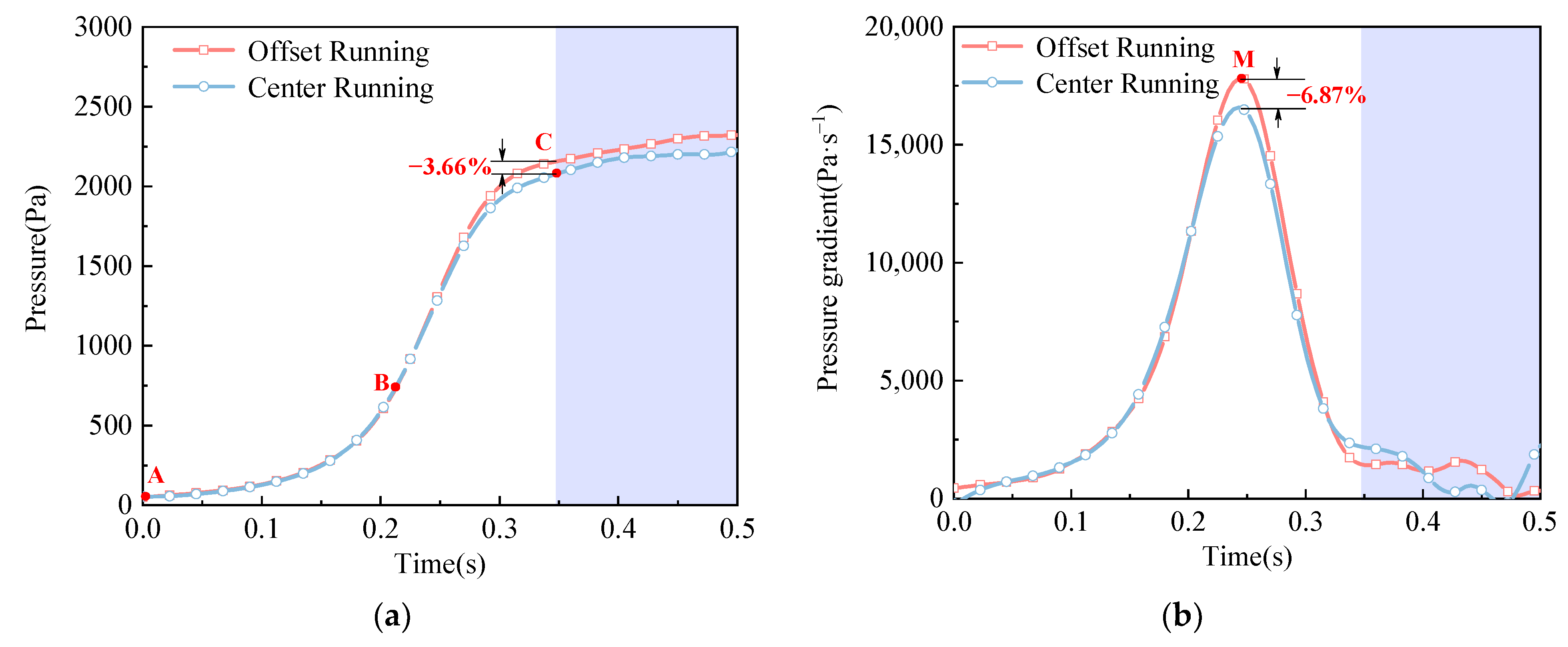
3.4.2. Comparison of the Waveforms

To investigate the effect of the train’s running position on the one-dimensional initial compression wave, Figure 23 compares the pressure distribution at the roof measurement point located 7Di away from the tunnel entrance for both cases. By comparing the wavefront pressure distribution at the measurement point, the differences in segment AB between the two cases are minimal, indicating that offset running has little impact on the pressure disturbances generated during open-air operation. However, there are differences in the disturbances generated within the tunnel; the amplitude of the initial compression wave in the center running case is 3.66% smaller than in the offset running case. In terms of pressure gradient, the time at which the maximum pressure gradient occurs is the same for both operating cases. However, the amplitude of the pressure gradient for the center running case is 6.87% smaller than that for the offset running case.

Based on the general equations of steady gas dynamics, Hara [21] developed a comprehensive formula for the overall pressure rise $\Delta p_{\mathrm{Hara}}$ across the compression wave:

$$\Delta p_{\mathrm{Hara}}={\displaystyle \frac{1}{2}}{\rho }_0{V}_{tr}^2{\displaystyle \frac{1-{(1-\beta )}^2}{(1-M_{tr})\left(M_{tr}+{(1-\beta )}^2\right)}},$$

(3)

where $M_{tr}$, $\beta$ represent the train’s Mach number and blockage ratio, respectively.

Table 2. The comparison of the initial wavefront amplitudes between the formula prediction and the simulation results.

Case	Offset Running	Center Running
Simulation (Pa)	2154.11	2075.30
Hara’s Formula (Pa)	2142.71
Relative Difference (%)	−0.53	3.25

compares the initial wavefront amplitudes between the formula prediction and the simulation results. The theoretical values align well with the numerical simulation results for both operating cases, with errors of −0.53% and 3.25% for offset and center operations, respectively.

4. Conclusions

In this study, based on the IDDES SST $k-\omega$ turbulence model, a three-dimensional numerical model was used to transiently simulate the initial compression wave induced by a 400 km/h high-speed train entering a tunnel. This work focused on analyzing the spatial and temporal distribution of the initial compression wave and its one-dimensional planar wave characteristics. The conclusions are as follows:

(1) Before the train enters the tunnel, the pressure at the measurement points inside the tunnel begins to rise. This is because the pressure disturbances generated by the train’s movement in the open air propagate into the tunnel. As the part of the streamlined nose with the maximum cross-sectional area change rate enters the tunnel, the resulting compression wave causes the largest pressure gradient at the measurement point;

(2) Pressure iso-surfaces can illustrate the process of the compression wave transitioning from three-dimensional characteristics to a one-dimensional planar wave. The pressure distribution near the train’s nose inside the tunnel exhibits significant three-dimensional features. When using lower pressure values, the pressure iso-surfaces can represent the compression wave in front of the train. The compression wave close to the train is oblique, while the compression wave farther from the train becomes a one-dimensional planar wave;

(3) The initial compression wave captured at the measurement points at a distance of 5Di (Di represents the equivalent diameter of the tunnel) from the tunnel portal has been fully characterized by one-dimensional features, which can provide a boundary input for the propagation of the initial compression wave towards the tunnel exit;

(4) Regarding the offset effect of the train, the high-pressure iso-surfaces show significant differences between the offset running and center running cases. Due to the constraints of the ground and tunnel walls, the high-pressure region exhibits an irregular spherical shape in offset running, while in the center running case, the tunnel walls impose no restriction on the development of the pressure iso-surface, the iso-surface gradually develops symmetrically from the center to both sides. Compared to the offset running case, the initial compression wave amplitude and pressure gradient amplitude induced by central running are reduced by 3.66% and 6.87%, respectively.

References

1. Dai, Z.; Li, T.; Zhang, W.; Zhang, J. Investigation on aerodynamic characteristics of high-speed trains with shields beneath bogies. J. Wind. Eng. Ind. Aerodyn. 2024, 246, 105666. [Google Scholar] [CrossRef]
2. Mou, R.; Chen, C.; Chen, C.; Zhang, Y. Analysis and control of high-speed train lateral vibration on the basis of a conditionally triggered model predictive control strategy. J. Mech. Sci. Technol. 2024, 38, 1703–1717. [Google Scholar] [CrossRef]
3. Baker, C.J. A review of train aerodynamics Part 1—Fundamentals. Aeronaut. J. 2014, 118, 201–228. [Google Scholar] [CrossRef]
4. Niu, J.; Sui, Y.; Yu, Q.; Cao, X.; Yuan, Y. Aerodynamics of railway train/tunnel system: A review of recent research. Energy Built Environ. 2020, 1, 351–375. [Google Scholar] [CrossRef]
5. Ozawa, S. Studies of micro-pressure wave radiated from a tunnel exit. Railw. Tech. Res. Rep. 1979, 1121, 1–92. (In Japanese) [Google Scholar]
6. Vardy, A.E. Generation and alleviation of sonic booms from rail tunnels. Proc. Inst. Civ. Eng.-Eng. Comput. Mech. 2008, 161, 107–119. [Google Scholar] [CrossRef]
7. Baron, A.; Molteni, P.; Vigevano, L. High-speed trains: Prediction of micro-pressure wave radiation from tunnel portals. J. Sound Vib. 2006, 296, 59–72. [Google Scholar] [CrossRef]
8. Zhang, G.; Kim, T.H.; Kim, D.H.; Kim, H.D. Prediction of micro-pressure waves generated at the exit of a model train tunnel. J. Wind. Eng. Ind. Aerodyn. 2018, 183, 127–139. [Google Scholar] [CrossRef]
9. Aoki, T.; Vardy, A.; Brown, J. Passive alleviation of micro-pressure waves from tunnel portals. J. Sound Vib. 1999, 220, 921–940. [Google Scholar] [CrossRef]
10. Fukuda, T.; Ozawa, S.; Iida, M.; Takasaki, T.; Wakabayashi, Y.; Miyachi, T. Propagation of Compression Wave in a Long Tunnel with Slab Tracks. Q. Rep. RTRI 2005, 46, 188–193. [Google Scholar] [CrossRef]
11. Tebbutt, J.; Vahdati, M.; Carolan, D.; Dear, J. Numerical investigation on an array of Helmholtz resonators for the reduction of micro-pressure waves in modern and future high-speed rail tunnel systems. J. Sound Vib. 2017, 400, 606–625. [Google Scholar] [CrossRef]
12. Kwon, H.-B.; Jang, K.-H.; Kim, Y.-S.; Yee, K.-J.; Lee, D.-H. Nose Shape Optimization of High-speed Train for Minimization of Tunnel Sonic Boom. JSME Int. J. Ser. C Mech. Syst. Mach. Elem. Manuf. 2001, 44, 890–899. [Google Scholar] [CrossRef]
13. Auvity, B.; Bellenoue, M. Effects of an opening on pressure wave propagation in a tube. J. Fluid Mech. 2005, 538, 269–289. [Google Scholar] [CrossRef]
14. Zhang, L.; Thurow, K.; Stoll, N.; Liu, H. Influence of the geometry of equal-transect oblique tunnel portal on com-pression wave and micro-pressure wave generated by high-speed trains entering tunnels. J. Wind. Eng. Ind. Aerodyn. 2018, 178, 1–17. [Google Scholar] [CrossRef]
15. Mashimo, S.; Nakatsu, E.; Aoki, T.; Matsuo, K. Attenuation and Distortion of a Compression Wave Propagating in a High-Speed Railwav Tunnel. JSME Int. J. Ser. B Fluids Therm. Eng. 1997, 40, 51–57. [Google Scholar] [CrossRef]
16. Wang, H.; Lei, B.; Bi, H.; Yu, T. Wavefront evolution of compression waves propagating in high speed railway tunnels. J. Sound Vib. 2018, 431, 105–121. [Google Scholar] [CrossRef]
17. Iyer, R.S.; Kim, D.H.; Kim, H.D. Propagation characteristics of compression wave in a high-speed railway tunnel. Phys. Fluids 2021, 33, 086104. [Google Scholar] [CrossRef]
18. Miyachi, T.; Ozawa, S.; Fukuda, T.; Iida, M.; Arai, T. A New Simple Equation Governing Distortion of Compression Wave Propagating Through Shinkansen Tunnel with Slab Tracks. J. Fluid Sci. Technol. 2013, 8, 462–475. [Google Scholar] [CrossRef]
19. Li, G.-Z.; Ye, X.; Deng, E.; Yang, W.-C.; Ni, Y.-Q.; He, H.; Ao, W.-K. Aerodynamic mechanism of a combined buffer hood for mitigating micro-pressure waves at the 400 km/h high-speed railway tunnel portal. Phys. Fluids 2023, 35, 126106. [Google Scholar] [CrossRef]
20. Kim, B.; Ahn, J.; Kwon, H. Numerical study of the effect of the tunnel hood on micro-pressure wave for increasing high-speed train operation speed. J. Mech. Sci. Technol. 2024, 38, 721–733. [Google Scholar] [CrossRef]
21. Hara, T. Aerodynamic Force Acting on a High Speed Train at Tunnel Entrance. Bull. JSME 1961, 4, 547–553. [Google Scholar] [CrossRef]
22. Howe, M.S. The compression wave produced by a high-speed train entering a tunnel. Proc. R. Soc. Lond. Ser. A Math. Phys. Eng. Sci. 1998, 454, 1523–1534. [Google Scholar] [CrossRef]
23. Howe, M.; Iida, M.; Fukuda, T. Influence of an unvented tunnel entrance hood on the compression wave generated by a high-speed train. J. Fluids Struct. 2003, 17, 833–853. [Google Scholar] [CrossRef]
24. Howe, M.S.; Iida, M.; Fukuda, T.; Maeda, T. Theoretical and experimental investigation of the compression wave generated by a train entering a tunnel with a flared portal. J. Fluid Mech. 2000, 425, 111–132. [Google Scholar] [CrossRef]
25. Howe, M.; Iida, M.; Maeda, T.; Sakuma, Y. Rapid calculation of the compression wave generated by a train entering a tunnel with a vented hood. J. Sound Vib. 2006, 297, 267–292. [Google Scholar] [CrossRef]
26. Howe, M.; Winslow, A.; Iida, M.; Fukuda, T. Rapid calculation of the compression wave generated by a train entering a tunnel with a vented hood: Short hoods. J. Sound Vib. 2007, 311, 254–268. [Google Scholar] [CrossRef]
27. Bellenoue, M.; Morinière, V.; Kageyama, T. Experimental 3-d simulation of the compression wave, due to train–tunnel entry. J. Fluids Struct. 2002, 16, 581–595. [Google Scholar] [CrossRef]
28. Wang, T.; Chen, J.; Wang, J.; Shi, F.; Zhang, L.; Qian, B.; Jiang, C.; Wang, J.; Wang, Y.; Yang, M. Three-dimensional characteristics of pressure waves induced by high-speed trains passing through tunnels. Acta Mech. Sin. 2024, 40, 323261. [Google Scholar] [CrossRef]
29. Kikuchi, K.; Iida, M.; Fukuda, T. Optimization of Train Nose Shape for Reducing Micro-Pressure Wave Radiated from Tunnel Exit. J. Low Freq. Noise Vib. Act. Control 2011, 30, 1–19. [Google Scholar] [CrossRef]
30. Ku, Y.C.; Rho, J.H.; Yun, S.H.; Kwak, M.H.; Kim, K.H.; Kwon, H.B.; Lee, D.H. Optimal cross-sectional area dis-tribution of a high-speed train nose to minimize the tunnel micro-pressure wave. Struct. Multidiscip. Optim. 2010, 42, 965–976. [Google Scholar] [CrossRef]
31. Miyachi, T.; Kikuchi, K.; Hieke, M. Multistep train nose for reducing micro-pressure waves. J. Sound Vib. 2021, 520, 116665. [Google Scholar] [CrossRef]
32. Kim, D.H.; Cheol, S.Y.; Iyer, R.S.; Kim, H.D. A newly designed entrance hood to reduce the micro pressure wave emitted from the exit of high-speed railway tunnel. Tunn. Undergr. Space Technol. 2020, 108, 103728. [Google Scholar] [CrossRef]
33. Okubo, H.; Miyachi, T.; Fukuda, T. Field test for micro-pressure wave reduction measurement by area optimization of windows of tunnel hoods. Proc. Inst. Mech. Eng. Part F J. Rail Rapid Transit 2022, 236, 1262–1270. [Google Scholar] [CrossRef]
34. Ma, W.; Fang, Y.; Li, T.; Shao, M. Alleviation Effects of Hoods at the Entrances and Exits of High-Speed Railway Tunnels on the Micro-Pressure Wave. Appl. Sci. 2024, 14, 692. [Google Scholar] [CrossRef]
35. Wang, T.; Feng, Z.; Lu, Y.; Gong, Y.; Zhu, Y.; Zhao, C.; Zhang, L.; Shi, F.; Wang, Y. Study on the mitigation effect of a new type of connected structure on micro-pressure waves around 400 km/h railway tunnel exit. J. Wind. Eng. Ind. Aerodyn. 2023, 240, 105510. [Google Scholar] [CrossRef]
36. Niu, J.; Zhou, D.; Liu, F.; Yuan, Y. Effect of train length on fluctuating aerodynamic pressure wave in tunnels and method for determining the amplitude of pressure wave on trains. Tunn. Undergr. Space Technol. 2018, 80, 277–289. [Google Scholar] [CrossRef]
37. Li, W.-H.; Liu, T.-H.; Martinez-Vazquez, P.; Xia, Y.-T.; Chen, Z.-W.; Guo, Z.-J. Aerodynamic effects on a railway tunnel with partially changed cross-sectional area. J. Cent. South Univ. 2022, 29, 2589–2604. [Google Scholar] [CrossRef]
38. Luo, J.; Wang, L.; Shang, S.; Li, F.; Guo, D.; Gao, L.; Wang, D. Study of unsteady aerodynamic performance of a high-speed train entering a double-track tunnel under crosswind conditions. J. Fluids Struct. 2023, 118, 103836. [Google Scholar] [CrossRef]
39. Wang, T.; Zhu, Y.; Tian, X.; Shi, F.; Zhang, L.; Lu, Y. Design method of the variable cross-section tunnel focused on improving passenger pressure comfort of trains intersecting in the tunnel. J. Affect. Disord. 2022, 221, 109336. [Google Scholar] [CrossRef]
40. Liu, Z.; Chen, G.; Zhou, D.; Wang, Z.; Guo, Z. Numerical investigation of the pressure and friction resistance of a high-speed subway train based on an overset mesh method. Proc. Inst. Mech. Eng. Part F J. Rail Rapid Transit 2021, 235, 598–615. [Google Scholar] [CrossRef]
41. Lv, D.; Niu, J.; Yao, H. Numerical study on transient aerodynamic characteristics of high-speed trains during the opening of braking plates based on dynamic-overset-grid technology. J. Wind. Eng. Ind. Aerodyn. 2023, 233, 105299. [Google Scholar] [CrossRef]
42. Hu, X.; Deng, Z.; Zhang, W. Effect of cross passage on aerodynamic characteristics of super-high-speed evacuated tube transportation. J. Wind. Eng. Ind. Aerodyn. 2021, 211, 104562. [Google Scholar] [CrossRef]
43. Liu, Z.; Zhou, D.; Soper, D.; Chen, G.; Hemida, H.; Guo, Z.; Li, X. Numerical investigation of the slipstream charac-teristics of a maglev train in a tunnel. Proc. Inst. Mech. Eng. Part F J. Rail Rapid Transit 2023, 237, 179–192. [Google Scholar] [CrossRef]
44. Xiang, X.; Xue, L.; Wang, B.; Zou, W. Mechanism and capability of ventilation openings for alleviating micro-pressure waves emitted from high-speed railway tunnels. J. Affect. Disord. 2018, 132, 245–254. [Google Scholar] [CrossRef]
45. Hu, X.; Deng, Z.; Zhang, J.; Zhang, W. Aerodynamic behaviors in supersonic evacuated tube transportation with different train nose lengths. Int. J. Heat Mass Transf. 2021, 183, 122130. [Google Scholar] [CrossRef]
46. Hu, X.; Deng, Z.; Zhang, J.; Zhang, W. Effect of tracks on the flow and heat transfer of supersonic evacuated tube maglev transportation. J. Fluids Struct. 2021, 107, 103413. [Google Scholar] [CrossRef]
47. Meng, S.; Meng, S.; Wu, F.; Li, X.; Zhou, D. Comparative analysis of the slipstream of different nose lengths on two trains passing each other. J. Wind. Eng. Ind. Aerodyn. 2020, 208, 104457. [Google Scholar] [CrossRef]
48. Dong, T.; Liang, X.; Krajnović, S.; Xiong, X.; Zhou, W. Effects of simplifying train bogies on surrounding flow and aerodynamic forces. J. Wind. Eng. Ind. Aerodyn. 2019, 191, 170–182. [Google Scholar] [CrossRef]
49. Muld, T.W.; Efraimsson, G.; Henningson, D.S. Flow structures around a high-speed train extracted using Proper Orthogonal Decomposition and Dynamic Mode Decomposition. Comput. Fluids 2012, 57, 87–97. [Google Scholar] [CrossRef]
50. Menter, F.R. Two-equation eddy-viscosity turbulence models for engineering applications. AIAA J. 1994, 32, 1598–1605. [Google Scholar] [CrossRef]
51. He, K.; Su, X.; Gao, G.; Krajnović, S. Evaluation of LES, IDDES and URANS for prediction of flow around a streamlined high-speed train. J. Wind. Eng. Ind. Aerodyn. 2022, 223, 104952. [Google Scholar] [CrossRef]
52. Niu, J.; Wang, Y.; Zhang, L.; Yuan, Y. Numerical analysis of aerodynamic characteristics of high-speed train with different train nose lengths. Int. J. Heat Mass Transf. 2018, 127, 188–199. [Google Scholar] [CrossRef]
53. Doi, T.; Ogawa, T.; Masubuchi, T.; Kaku, J. Development of an experimental facility for measuring pressure waves generated by high-speed trains. J. Wind. Eng. Ind. Aerodyn. 2010, 98, 55–61. [Google Scholar] [CrossRef]
54. Iida, M.; Tanaka, Y.; Kikuchi, K.; Fukuda, T. Pressure Waves Radiated Directly from Tunnel Portals at Train Entry or Exit. Q. Rep. RTRI 2001, 42, 83–88. [Google Scholar] [CrossRef]
Figure 1. Schematic diagram of micro-pressure wave formation. It is divided into four processes: the generation of pressure wave, propagation of pressure wave, radiation of micro pressure wave, and transmission of micro pressure wave to receiver.
Applsci 14 07208 g001
Figure 2. Dimensions of the train and tunnel model: (a) the side-view of the train model; (b) the streamlined nose of the train; (c) the powered bogie model; (d) the trailer bogie model; (e) the train/tunnel model of the offset running case; (f) the train/tunnel model of the center running case.
Applsci 14 07208 g002
Figure 3. The distribution of the cross-sectional area and change rate of the streamlined train nose along the flow direction.
Applsci 14 07208 g003
Figure 4. Schematic diagrams of the computational domain and boundary conditions at t = 0 s: (a) side-view; (b) top-view (not to scale).
Applsci 14 07208 g004
Figure 5. The visualization of the mesh at a specific moment during the process of a train entering the tunnel: (a) the mesh refinement distribution of the longitudinal center section of the train; (b) a locally magnified view near the head car; (c) a locally magnified view near the tail car; (d) the prism layer mesh of the tunnel wall; (e) the prism layer mesh of the train wall.
Applsci 14 07208 g005
Figure 6. The train model used in moving model experiments: (a) side view; (b) top-view; (c) three-dimensional view.
Applsci 14 07208 g006
Figure 7. (a) The distribution of the tunnel/train model and (b) the arrangement of the measurement points in the moving model experiments.
Applsci 14 07208 g007
Figure 8. Comparison of the numerical simulation results in three sets of meshes with the experimental results at point P1: (a) Pressure coefficient-time history; (b) Pressure coefficient gradient-time history.
Applsci 14 07208 g008
Figure 9. The pressure fluctuation signature at a fixed position in a tunnel [4].
Applsci 14 07208 g009
Figure 10. The basic characteristics of the initial compression wave: (a) Trajectory diagram of the head car and its induced compression waves; (b) time history of initial compression wave and pressure gradient at roof measurement points located 5Di and 7Di away from the tunnel entrance.
Applsci 14 07208 g010
Figure 11. The characteristics of pressure distribution inside the tunnel at 0 s: (a) The pressure distribution of the train’s surface and the tunnel wall; (b) the three-dimensional distribution of pressure iso-surfaces at 200 Pa, 400 Pa, and 800 Pa; (c) the pressure distribution across cross-sections from 1Di to 8Di away from the tunnel entrance.
Applsci 14 07208 g011
Figure 12. The characteristics of pressure distribution inside the tunnel at 0.0675 s: (a) The pressure distribution of the train’s surface and the tunnel wall; (b) the three-dimensional distribution of pressure iso-surfaces at 400 Pa, 800 Pa, and 1600 Pa; (c) the pressure distribution across cross-sections from 1Di to 8Di away from the tunnel entrance.
Applsci 14 07208 g012
Figure 13. The characteristics of pressure distribution inside the tunnel at 0.135 s: (a) The pressure distribution of the train’s surface and the tunnel wall; (b) the three-dimensional distribution of pressure iso-surfaces at 500 Pa, 1000 Pa, and 2000 Pa; (c) the pressure distribution across cross-sections from 1Di to 8Di away from the tunnel entrance.
Applsci 14 07208 g013
Figure 14. Comparison of maximum and minimum pressures across different cross-sections from the tunnel entrance at (a) 0 s; (b) 0.0675 s; (c) 0.135 s; (d) 0.2025 s; (e) 0.27 s.
Applsci 14 07208 g014
Figure 15. The layout of pressure measurement points inside the tunnel: (a) front view; (b) top view.
Applsci 14 07208 g015
Figure 16. Comparison of the initial compression waves at different points in the 3Di cross-section: (a) pressure–time history curves; (b) pressure gradient–time history curves.
Applsci 14 07208 g016
Figure 17. Comparison of the initial compression waves at different points in the 4Di cross-section: (a) pressure–time history curves; (b) pressure gradient–time history curves.
Applsci 14 07208 g017
Figure 18. Comparison of the initial compression waves at different points in the 5Di cross-section: (a) Pressure–time history curves; (b) Pressure gradient–time history curves.
Applsci 14 07208 g018
Figure 19. Comparison of the initial compression waves at different points in the 6Di cross-section: (a) pressure–time history curves; (b) 0ressure gradient–time history curves.
Applsci 14 07208 g019
Figure 20. Comparison of the velocity line integral convolution of the z = 0 m section colored by velocity magnitude during the process of the head car entering the tunnel.
Applsci 14 07208 g020
Figure 21. Comparison of the velocity line integral convolution of the y = 0 m section colored by velocity magnitude during the process of the head car entering the tunnel.
Applsci 14 07208 g021
Figure 22. Comparison of the three-dimensional distribution of pressure iso-surfaces at (a) 2400 Pa, (b) 1800 Pa.
Applsci 14 07208 g022
Figure 23. Comparison of the initial compression waves at point 3 in the 7Di cross-section: (a) pressure–time history; (b) pressure gradient–time history.
Applsci 14 07208 g023