An Assessment Method for the Step-Down Stress Accelerated Degradation Test Considering Random Effects and Detection Errors

Abstract

The step-stress accelerated degradation test (ADT) provides a feasible method for assessing the storage life of high-reliability, long-life products. However, this method results in a slower rate of performance degradation at the beginning of the test, significantly reducing the test efficiency. Therefore, this article proposes an assessment method for the step-down stress ADT that considers random effects and detection errors (SDRD). Firstly, a new Inverse Gaussian (IG) model is proposed. The model introduces the Gamma distribution to characterize the randomness of the product degradation path and uses the normal distribution to describe the detection errors of performance parameters. In addition, to solve the problem that the likelihood function of the IG model is complex and has no explicit expression, the Monte Carlo (MC) method is used to estimate unknown parameters of the model. This approach enhances computational accuracy and efficiency. Finally, to verify the effectiveness of the SDRD method, it is applied to the step-down stress ADT data from a specific missile tank to assess its storage life. Comparing the life assessment results of different methods, the conclusion shows that the SDRD method is more effective for assessing the storage life of high-reliability, long-life products.

1. Introduction

For high-reliability, long-life products with the characteristics of long-term storage and single-use, the majority of their lifecycle from manufacturing to deployment is spent in the storage period [1]. During long-term storage, products are subject to various external environmental influences that can lead to changes in performance. These changes may ultimately affect their operational reliability. Therefore, storage reliability has become one of the key performance indicators for products, which is directly related to the maintenance, management, and operational effectiveness of products. A reasonable modeling analysis of the storage reliability of the product helps to ensure that the product plays the expected role at the critical time and achieves the goal of reliable operation [2,3,4].

Traditional accelerated life test methods mainly rely on failure life data. However, high-reliability, long-life electromechanical products cannot obtain sufficient life data within a short time for life prediction [5,6,7]. At this time, it is difficult to obtain effective assessment results using traditional accelerated life test methods. In fact, product failure is caused by gradual performance degradation, and the process of performance degradation contains a wealth of reliability information. Moreover, the accelerated degradation test (ADT) does not require products to be accelerated to failure, which can significantly shorten the test time. This is particularly beneficial for high-reliability, long-life products that are expensive to manufacture, as it can effectively reduce test costs. Therefore, ADT methods based on performance degradation provide a new approach for assessing the storage life of high-reliability, long-life products [8,9]. At present, the more popular ADT methods mainly include the constant-stress accelerated degradation test (CSADT) and the step-stress accelerated degradation test (SSADT) [10]. The CSADT is relatively mature, but it requires a long testing time and a large sample size of test products. Compared to the CSADT, the SSADT can significantly reduce the number of test samples by several times. Moreover, as the stress level gradually increases, the trend of product performance degradation becomes more obvious. However, due to the low initial stress level, the rate of performance decline at the beginning of the test is slow, which greatly reduces the efficiency of the accelerated test. Based on this, Zhang et al. proposed a step-down stress accelerated degradation test (SDSADT) method, which suggested that changing the sequence of stress application could significantly enhance test efficiency [11]. Subsequently, Cai et al. proposed step-up-stress ADT and SDSADT for studying the thermal degradation kinetics of light-emitting diode (LED) lamps. The results indicated that the SDSADT could effectively alleviate the initial increase in the optical parameters of LED lamps [12]. Therefore, this article mainly focuses on the SDSADT method, emphasizing performance degradation.

Degradation trajectory models are widely used in early performance degradation-based reliability research due to their intuitiveness and ease of understanding. For example, Qi et al. established the degradation trajectory equation for the dual-stress accelerated degradation process to assess the storage life of power switching transistors [13]. The following year, Hong et al. extended the general degradation trajectory equation to the case of varying environmental stress and established a general degradation trajectory equation under varying environmental stress to describe the impact of random stresses [14]. Subsequently, Liu et al. proposed a new random effects model based on reference [14] to deal with degradation data under irregular time-varying environmental stress conditions. This model provided a new theory and method for modeling the degradation path of lithium-ion cells [15]. The degradation trajectory model can be used to establish the life model of the product intuitively. However, during the storage process, due to the influence of environmental stresses such as temperature, humidity, and salt spray, the degradation process of individual products is uncertain. At this time, reliability models based on degradation trajectories perform poorly in describing and explaining the randomness of product degradation paths. Stochastic process models have good performance in describing the time-varying uncertainty of products, so they are widely used in product performance degradation analysis. Specifically, Tang et al. studied parameter estimation methods based on intermediate data using the Wiener process, and the lifetime distribution function estimation method proposed is more accurate than both the standard and modified maximum likelihood estimation (MLE) methods [16]. The Wiener process is suitable for describing non-monotonic performance degradation processes with increasing or decreasing trends, while the Gamma process and Inverse Gaussian (IG) process are suitable for describing monotonic continuous degradation processes. Aiming at monotonic continuous degradation processes, Wang et al. proposed the MLE method based on the IG model and used the EM algorithm to calculate estimates of the unknown parameters [17]. Zhang et al. also used the IG process model for modeling energy pipelines. At the same time, considering the possibility of detection errors in the detection results, Bayes was used to estimate the model parameters [18]. On this basis, Peng et al. proposed a general Bayesian framework for the degradation analysis of IG process models and focused on the applicability of Bayesian methods in the degradation analysis of IG process models [19]. Tsai et al. proposed a nonlinear Gamma process model based on the time transfer function and used the MLE method to estimate model parameters [20]. Kou et al. focused on the randomness of product degradation paths and proposed a novel assessment method based on the IG process to analyze and predict the results of the SDSADT [21].

From the above literature, it is known that stochastic process models are widely applied and have achieved certain successes in ADT data processing. However, existing methods rarely consider the following two situations: First, the detection equipment is affected by noise and disturbance, and the detection results have detection errors. Second, the degradation paths of different products exhibit randomness and difference. In addition, due to the low initial stress level of the SSADT, the rate of performance decline at the beginning of the test is slow. This greatly reduces the efficiency of the accelerated test. By applying high stress to the product at the beginning of the SDSADT, the reliability information of the product can be obtained in a shorter time and the test efficiency can be improved. Based on this, this article proposes a storage life assessment method for the SDSADT that considers random effects and detection errors and applies it to the SDSADT data from a specific missile tank to assess its storage life. The main contributions of this article are as follows.

(1)

This article proposes a new method for assessing storage life under the SDSADT to solve the problem of slow product performance degradation at the beginning of the step-stress ADT. This article mainly focuses on the assessment method for the storage life of high-reliability and long-life products under the SDSADT.

(2)

A new IG performance degradation model is proposed. This model introduces the Gamma distribution to characterize the randomness of and difference in the degradation paths of different products and uses the normal distribution to describe the detection errors of performance parameters. This model can solve the problem of the product storage life assessment caused by random effects and detection errors.

(3)

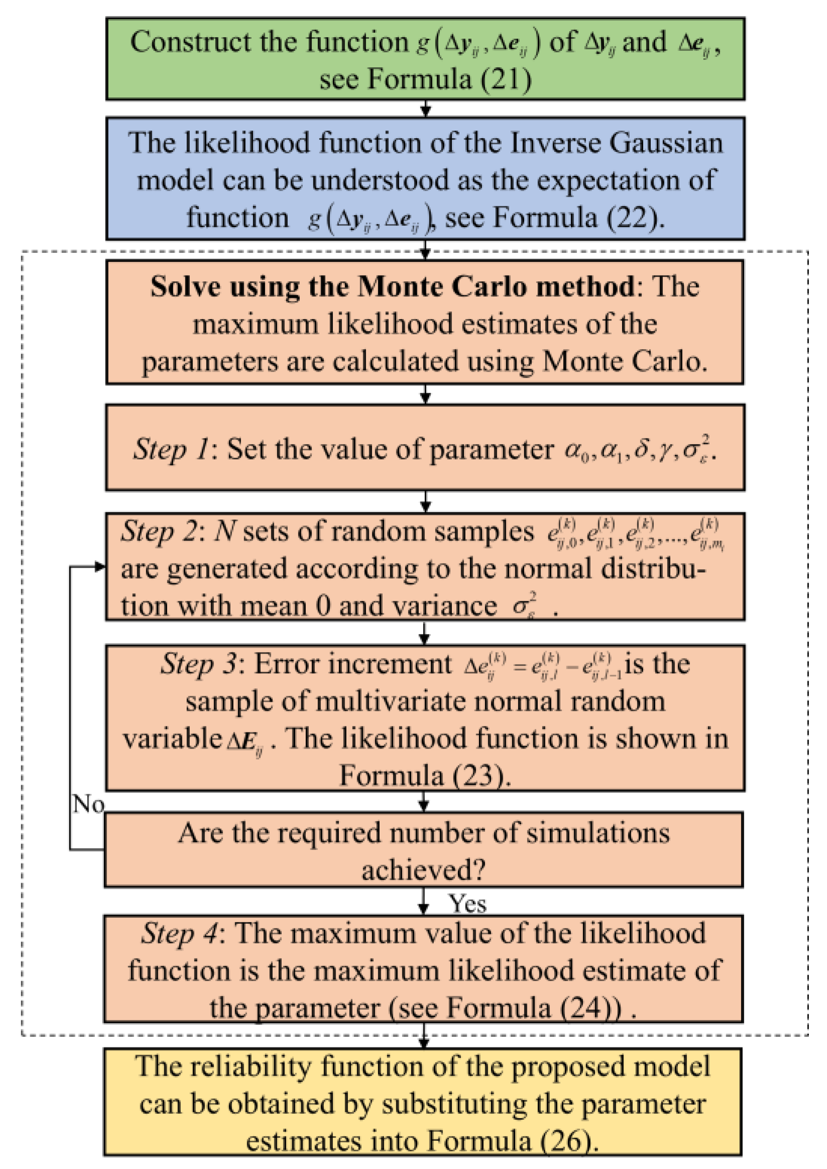
The Monte Carlo (MC) technique is employed to estimate the unknown parameters in the IG model to solve the problem that the calculation of the likelihood function is complicated and there is no explicit expression. This method can improve the calculation accuracy and efficiency.

(4)

Parameter estimation and storage life assessment are carried out on the SDSADT data from a specific missile tank to verify the effectiveness and feasibility of the proposed method.

2. Theoretical Background

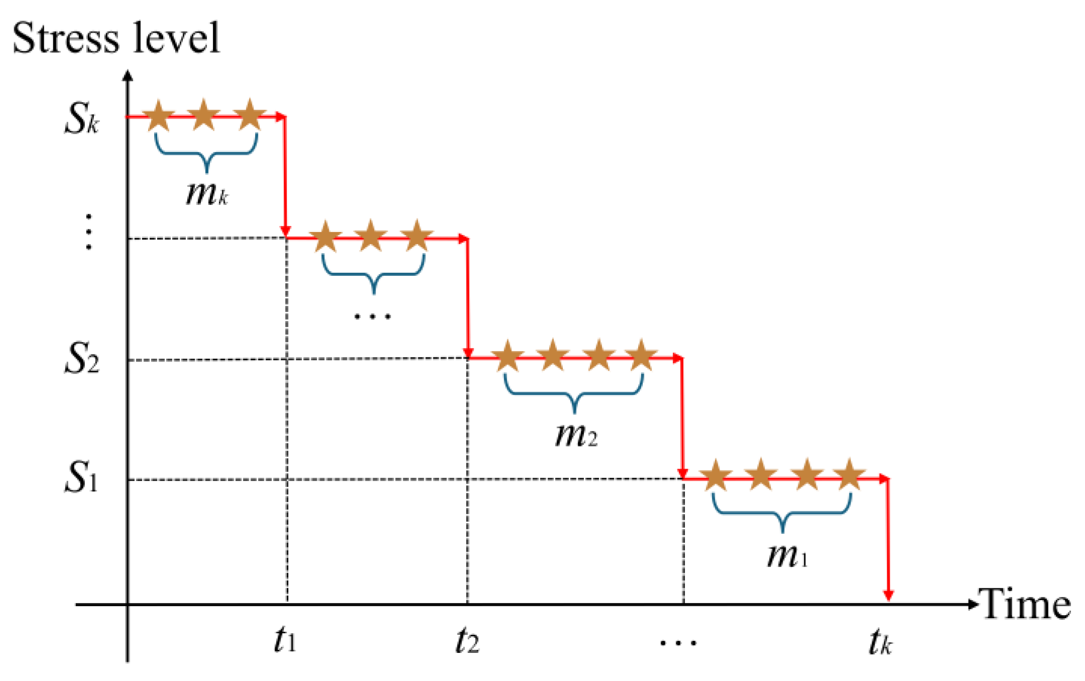
2.1. Step-Down Stress Accelerated Degradation Test

The SDSADT is a common reliability test method used to evaluate the performance degradation of products under various stress conditions. The advantage of this method lies in its ability to obtain the reliability information of products under actual storage conditions within a shorter time, and to assist in identifying the potential failure modes and failure mechanisms of the products [22]. There are $k$ accelerating stress levels $S_i(i=1,2,\dots ,k)$, and $S_k>S_{k-1}>\cdots >S_1>S_0$. In the SDSADT, $S_k$ is assumed to be the initial stress level and $S_0$ is the normal stress level. $m_i$ is the number of detections at the stress level $S_i$. Usually, the number of stress levels $k$ should not be less than three. At the beginning of the test, the samples are subjected to the ADT under stress level $S_k$, during which the samples are taken out for $m_k$ performance tests. After a time $t_1$, the stress level is reduced to $S_{k-1}$, and the samples are then subjected to the ADT under stress level $S_{k-1}$, during which the samples are taken out for $m_{k-1}$ performance tests. The stress level is sequentially reduced until a certain termination time is reached. The variation trend of stress level over time in the SDSADT is shown in Figure 1.

The storage life of products is mainly influenced by temperature and humidity. However, during storage, measures such as sealed packaging are often used to eliminate the impact of humidity on storage life. Therefore, this article employs a constant-humidity step-down temperature stress ADT. The Arrhenius model is commonly used when the temperature serves as the accelerating stress. The Arrhenius model describes the relationship between temperature stress and degradation paths. This actually reflects the fundamental idea of the Boltzmann distribution, which is the relationship between the probability of each state in the system and the energy and temperature. Therefore, the Arrhenius model can be seen as an application of the Boltzmann distribution under specific conditions. Based on the degradation characteristics of product performance parameters, the model is defined as follows [23]:

$$h(S)={\xi }_0\cdot e^{-{\displaystyle \frac{E}{KS}}}$$

(1)

where ${\xi }_0$ is the constant, determined by the product geometry and testing method. $E$ is the activation energy, which is related to the material. $K$ is the Boltzmann constant, with a value of $8.6\times {10}^{-5}$ eV/°C. $S$ is the temperature stress level in Kelvin. The exponential term $e^{-{\displaystyle \frac{E}{KS}}}$ in Formula (1) can be regarded as the Boltzmann factor, which represents the probability that the system is in a high energy state (i.e., needs to overcome activation energy $E$) at a given temperature $S$.

Accelerated stress levels can be standardized as follows:

$$x_i={\displaystyle \frac{1/S_0-1/S_i}{1/S_0-1/S_k}}$$

(2)

It can be seen from (2) that $x_0=0$, $x_k=1$, and $0<x_i\le 1(i=1,2,\dots ,k)$. Then, Formula (1) can be changed to the following:

$$h(x)=\exp ({\alpha }_0+{\alpha }_{1}x)$$

(3)

where ${\alpha }_0=\ln {\xi }_0-{\displaystyle \frac{E}{K{S}_0}}=\ln {\xi }_0-{\displaystyle \frac{\omega }{S_0}}$ and ${\alpha }_1={\displaystyle \frac{E}{K}}(1/S_0-1/S_k)=\omega (1/S_0-1/S_k)$. According to Formula (3), $h(x)$ is the monotone increasing function of stress level $x$. The higher the stress level, the more obvious the product degradation path. Taking $y_1=h(x_1)$ and $y_2=h(x_2)$, the geometric mean of $y_1$ and $y_2$ will be obtained at the arithmetic mean point of $x_1$ and $x_2$.

2.2. Life Assessment Method Based on IG Process for Accelerated Degradation Test

Without considering the random factors of the product degradation path, assuming that $\left\{Y(t),t\ge 0\right\}$ represents the product degradation and that $Y(t)$ conforms to the IG process, then $Y(t)$ has the following three characteristics:

(1)

The value of $Y(0)$ is always 0.

(2)

For any $0<t_1<t_2<t_3<t_4$, $Y(t_4)-Y(t_3)$ and $Y(t_2)-Y(t_1)$ are independent degradation increments.

(3)

For any $0\le s<t$, $Y(t)-Y(s)$ follows the IG process with mean $\mu \Delta \Lambda$ and variance ${\mu }^3\Delta \Lambda /\lambda$, which is denoted as $Y(t)-Y(s)~IG\left(\mu \Delta \Lambda ,\lambda {\left(\Delta \Lambda \right)}^2\right)$. Here, $\mu$ and $\lambda$ are constants. $\Delta \Lambda =\Lambda \left(t\right)-\Lambda \left(s\right)$, $\Lambda \left(0\right)=0$, and $\Lambda (\cdot )$ is the monotone increasing function of time $t$.

Based on the above three characteristics, the IG process model for $Y(t)$ can be established. Then, the MLE method is used to calculate the model parameters $\mathit{\theta }={\left(\mu ,\lambda \right)}^{\prime }$, thereby obtaining its reliability function. The specific details are as follows: It is assumed that the degradation amount $Y(t)$ follows the IG process with mean $\mu \Lambda \left(t\right)$ and variance ${\mu }^3\Lambda \left(t\right)/\lambda$, which is denoted as $Y\left(t\right)~IG\left(\mu \Lambda \left(t\right),\lambda {\Lambda }^2\left(t\right)\right)$. Here, $\mu$ is the degradation rate. $\lambda$ has no direct physical significance. Under the stress level $S_i$, $\lambda$ is constant, and the mean $\mu \Lambda \left(t\right)$ and variance ${\mu }^3\Lambda \left(t\right)/\lambda$ of $Y(t)$ are increasing. Therefore, let $\mu =h\left(S\right)$, where $h\left(S\right)$ is a function of the stress level and the product performance degradation. Then, the probability density function (PDF) of $Y(t)$ is as follows:

$$f\left(y\left(t\right)|h\left(x\right),\lambda \right)=\sqrt{{\displaystyle \frac{\lambda {\Lambda }^2\left(t\right)}{2\pi y{\left(t\right)}^3}}}\exp \left[-{\displaystyle \frac{\lambda {\left(y\left(t\right)-h\left(x\right)\Lambda \left(t\right)\right)}^2}{2h{\left(x\right)}^{2}y\left(t\right)}}\right]$$

(4)

It is assumed that under stress level $S_i$, the degradation amount of product $j$ at the time $t_l$ is $Y_{ij}\left(t_l\right),\left(i=1,2,\dots ,k;j=1,2,\dots ,n;l=1,2,\dots ,m_i\right)$. Here, $k$ represents the number of stress levels, $n$ represents the number of test products, and $m_i$ represents the detection number under stress level $S_i$. Then, the degradation increment of products is $\Delta y_{ij,l}=Y_{ij,l}-Y_{ij,l-1}$, and the increment of the monotone increasing function is ${\Lambda }_{ij,l}\left(t\right)=\Lambda \left(t_{ij,l}\right)-\Lambda \left(t_{ij,l-1}\right)$. Therefore, the likelihood function of the accelerated degradation model based on the IG process is as follows:

$$L\left(\mathit{\theta }\right)=\prod _{j=1}^n\prod _{i=1}^k\prod _{l=1}^{m_i}f\left(\Delta y_{ij,l};\mathit{\theta }\right)=\prod _{j=1}^n\prod _{i=1}^k\prod _{l=1}^{m_i}\left(\sqrt{{\displaystyle \frac{\lambda {\left({\Lambda }_{ij,l}\right)}^2}{2\pi \Delta y_{ij,l}^3}}}\times \exp \left[-{\displaystyle \frac{\lambda {\left(\Delta y_{ij,l}-e^{{\alpha }_0+{\alpha }_1{x}_i}{\Lambda }_{ij,l}\right)}^2}{2e^{2\left({\alpha }_0+{\alpha }_1{x}_i\right)}\Delta y_{ij,l}}}\right]\right)$$

(5)

where $\Lambda (\cdot )$ is a monotone increasing function of time $t$, indicating that the cumulative degradation effect of the product is proportional to time. The value of $\Lambda (\cdot )$ can be determined based on the personal experience of reliability engineers, knowledge of failure physics, handbooks, etc. [24]. In this article, $\Lambda \left(t\right)=t$. This provides a simplified linear accumulation assumption for the model, where the passage of time directly reflects the increase in the cumulative degradation effect. θ is the unknown parameter. Therefore, the log-likelihood function can be expressed as follows:

$$\ln L\left(\mathit{\theta }\right)={\displaystyle \sum _{j=1}^n{\displaystyle \sum _{i=1}^k{\displaystyle \sum _{l=1}^{m_i}\left(\frac{\ln \lambda }{2}+\ln t_{ij,l}-\frac{\lambda {\left(y_{ij,l}{e}^{-{\alpha }_0-{\alpha }_1{x}_i}-t_{ij,l}\right)}^2}{2y_{ij,l}}\right)}}}$$

(6)

where $\mathit{\theta }={\left({\alpha }_0,{\alpha }_1,\lambda \right)}^{\prime }$ can be solved by the MLE method.

In reliability degradation that follows the IG process, the product life $T_{D_f}$ can be defined as the time when the degradation $Y(t)$ first reaches the failure threshold $D_f$:

$$T_{D_f}=\inf \left\{t|Y\left(t\right)\ge D_f\right\}$$

(7)

The cumulative distribution function (CDF) of product life is the probability that the degradation $Y(t)$ exceeds the failure threshold $D_f$. Therefore, the CDF of the product life $T_{D_f}$ is as follows:

$$F_{T_{D_f}}\left(t\right)=P\left(T_{D_f}\le t\right)=1-\Phi \left[\sqrt{{\displaystyle \frac{\widehat{\lambda }}{D_f}}\left({\displaystyle \frac{D_f}{e^{\left({\widehat{\alpha }}_0+{\widehat{\alpha }}_{1}x\right)}}}-t\right)}\right]-\exp \left({\displaystyle \frac{2\widehat{\lambda }t}{e^{\left({\widehat{\alpha }}_0+{\widehat{\alpha }}_{1}x\right)}}}\right)\Phi \left[-\sqrt{{\displaystyle \frac{\widehat{\lambda }}{D_f}}\left({\displaystyle \frac{D_f}{e^{\left({\widehat{\alpha }}_0+{\widehat{\alpha }}_{1}x\right)}}}+t\right)}\right]$$

(8)

where $\Phi [\cdot ]$ is the CDF of the standard normal distribution. The CDF $F\left(t;\lambda ,\mu \right)$ of the general IG distribution can be expressed as $F\left(t;\lambda ,\mu \right)=\Phi \left(z\right)=\Phi \left(\sqrt{{\displaystyle \frac{\lambda }{t}}}\left({\displaystyle \frac{t}{\mu }}-1\right)\right)$. To simplify the calculation of the CDF of the IG distribution, the properties and calculation methods of the standard normal distribution can be used to analyze and assess the storage life of products. Formula (8) uses the mathematical connection between the IG distribution and the normal distribution to simplify the calculation.

Therefore, the reliability function is as follows:

$$\begin{array}{ll}R\left(t\right)& =P\left(T_D>t\right)=P\left(Y\left(t\right)\le D\right)=1-F_{T_D}\left(t\right)\\ & =\Phi \left[\sqrt{{\displaystyle \frac{\widehat{\lambda }}{D}}\left({\displaystyle \frac{D}{e^{\left({\widehat{\alpha }}_0+{\widehat{\alpha }}_{1}x\right)}}}-t\right)}\right]+\exp \left({\displaystyle \frac{2\widehat{\lambda }t}{e^{\left({\widehat{\alpha }}_0+{\widehat{\alpha }}_{1}x\right)}}}\right)\Phi \left[-\sqrt{{\displaystyle \frac{\widehat{\lambda }}{D}}\left({\displaystyle \frac{D}{e^{\left({\widehat{\alpha }}_0+{\widehat{\alpha }}_{1}x\right)}}}+t\right)}\right]\end{array}$$

(9)

3. Proposed Method

3.1. Model Assumption

To solve the problem that the degradation rate of products is slow at the beginning of the step-stress ADT, an assessment method for the SDSADT considering random effects and detection errors is proposed in this article. This article is based on the following three assumptions:

(1)

In the SDSADT, the degradation path of the product follows the IG process. Without loss of generality, it is assumed that the performance degradation increases monotonically with time.

(2)

The failure mechanism of the product under accelerated stress levels is unchanged and the same as under normal stress levels.

(3)

The remaining life of the product depends only on the current stress level and the parts that have accumulated degradation. It has nothing to do with the accumulation method [25].

Based on the above assumptions, this article proposes a new product storage life assessment method under the SDSADT. Firstly, the proposed method takes into account the effects of factors such as material and processing and introduces the Gamma distribution to characterize the randomness of and difference in the product degradation path. Secondly, due to the influence of uncertain factors such as detection equipment and environment, there are detection errors in the detection results. Therefore, the normal distribution is used to describe the detection errors of performance parameters. Based on this foundation, the MC method is used to estimate the model parameters and reliability. Compared with traditional parameter estimation methods, this approach can significantly improve calculation accuracy and efficiency.

3.2. IG Model Considering Random Effects and Detection Errors

In this section, a new IG process model is proposed that takes into account random effects and detection errors. The specific details are as follows:

Inspired by the literature [26], the Gamma distribution is introduced to characterize the randomness of and difference in the product degradation path to solve the problem posed by random effects on the product storage life assessment. It is assumed that $\lambda$ follows the Gamma distribution, that is, $\lambda \sim Gamma\left(\delta ,{\gamma }^{-1}\right),\left(\delta ,\gamma >0\right)$. Its PDF can be expressed as follows:

$$g\left(\lambda ;\delta ,\gamma \right)={\displaystyle \frac{{\gamma }^{\delta }{\lambda }^{\delta -1}}{\Gamma \left(\delta \right)}}\exp \left(-\gamma \lambda \right)I_{\left(0,\infty \right)}\left(\lambda \right),\lambda >0$$

(10)

where $\Gamma \left(\delta \right)$ is the Gamma function and $\Gamma \left(\delta \right)={\displaystyle {\int }_0^{\infty }{\lambda }^{\delta -1}}{e}^{-\lambda }d\lambda$, $I_{\left(0,\infty \right)}\left(\lambda \right)=\{\begin{array}{l}1,x\in \left(0,\infty \right)\\ 0,x\notin \left(0,\infty \right)\end{array}$. Combining Formulas (4) and (10), the PDF of $Y(t)$ is as follows:

$$f\left(y\left(t\right)|h\left(x\right),\delta ,\gamma \right)={\displaystyle \frac{\Gamma \left(\delta +1/2\right)}{\Gamma \left(\delta \right)}}{\gamma }^{\delta }\sqrt{{\displaystyle \frac{{\Lambda }^2\left(t\right)}{2\pi y{\left(t\right)}^3}}}\times {\left[\gamma +{\displaystyle \frac{{\left(y\left(t\right)-h\left(x\right)\Lambda \left(t\right)\right)}^2}{2h{\left(x\right)}^{2}y\left(t\right)}}\right]}^{-\delta -1/2}$$

(11)

where the mean of $Y(t)$ is $\mu \Lambda \left(t\right)$, the variance is $\gamma {\mu }^3\Lambda \left(t\right)/\left(\delta -1\right)$, and $\mu =h\left(x\right),\delta >1$. The likelihood function for the IG process model considering random effects is as follows:

$$L\left(\mathit{\theta }\right)=\prod _{j=1}^n\prod _{i=1}^k\prod _{l=1}^{m_i}f\left(\Delta y_{ij,l};\mathit{\theta }\right)=\prod _{j=1}^n\prod _{i=1}^k\prod _{l=1}^{m_i}{\displaystyle \frac{\Gamma \left(\delta +1/2\right)}{\Gamma \left(\delta \right)}}{\gamma }^{\delta }\sqrt{{\displaystyle \frac{\Delta t_{ij,l}^2}{2\pi \Delta y_{ij,l}^3}}}\times {\left[\gamma +{\displaystyle \frac{{\left(\Delta y_{ij,l}-h\left(x_i\right)\Delta t_{ij,l}\right)}^2}{2h{\left(x_i\right)}^2\Delta y_{ij,l}}}\right]}^{-\delta -1/2}$$

(12)

where $\mathit{\theta }={\left({\alpha }_0,{\alpha }_1,\delta ,\gamma \right)}^{\prime }$ is the unknown parameter.

Therefore, its logarithmic likelihood function is as follows:

$$\begin{array}{ll}\ln L\left(\mathit{\theta }\right)={\displaystyle \sum _{j=1}^n}{\displaystyle \sum _{i=1}^k}{\displaystyle \sum _{l=1}^{m_i}}& \{\ln \Gamma \left(\delta +m_i/2\right)-\ln \Gamma \left(\delta \right)\times \delta \ln \gamma +\left(\ln \Delta t_{ij,l}-3/2\times \ln \Delta y_{ij,l}\right)\\ & -\left(\delta +m_i/2\right)\times \ln \left[\gamma +{\displaystyle \frac{{\left(\Delta y_{ij,l}-e^{{\widehat{\alpha }}_0+{\widehat{\alpha }}_1{x}_i}\Delta t_{ij,l}\right)}^2}{2e^{2{\widehat{\alpha }}_0+2{\widehat{\alpha }}_1{x}_i}\Delta y_{ij,l}}}\right]\}\end{array}$$

(13)

Considering the influence of uncertain factors such as detection equipment and environment, there are detection errors in the detection results. Therefore, this article uses the normal distribution to describe the detection errors of performance parameters. Assume $Y_{ij,l}$ is the degradation detected value of the $j$-th sample at the time $t_l$ under stress level $S_i$, where $i=1,2,\dots ,k;j=1,2,\dots ,n;l=1,2,\dots ,m_i$. After the ADT, the true value of the product degradation path is $X_{ij,l}$, and then there is the following relationship between the detected value and the true value:

$$Y_{ij,l}=X_{ij,l}+E_{ij,l}$$

(14)

where $E_{ij,l}$ is the detection error, and $E_{ij,l}$ follows the normal distribution with mean 0 and standard deviation ${\sigma }_{\epsilon }$. Let $\Delta y_{ij,l}=y_{ij,l}-y_{ij,l-1}$ be the increment of the two detection values, according to Formula (14), it is known that

$$\Delta y_{ij,l}=\Delta x_{ij,l}+\Delta e_{ij,l}$$

(15)

where $\Delta e_{ij,l}=e_{ij,l}-e_{ij,l-1}$ is the increment of the detection error. For the $j$-th sample, $\Delta {\mathit{e}}_{ij}={\left(\Delta e_{ij,1},\Delta e_{ij,2},\dots ,\Delta e_{ij,m_i}\right)}^T$ is sample of random vector $\Delta {\mathit{E}}_{ij}={\left(E_{ij,1}-E_{ij,0},E_{ij,2}-E_{ij,1},\dots ,E_{ij,m_i}-E_{ij,m_i-1}\right)}^T$. Let ${\mathit{E}}_{ij}={\left(E_{ij,0},E_{ij,1},\dots ,E_{ij,m_i}\right)}^T$, ${\mathit{E}}_{ij}$ follows the multivariate normal distribution with mean 0 and variance ${\sigma }_{\epsilon }^2{\mathit{I}}_{m_i+1}$, and ${\mathit{I}}_{m_i+1}$ is the $m_{i+1}$-dimensional identity matrix. Let $\Delta {\mathit{E}}_{ij}=\mathit{J}{\mathit{E}}_{ij}$, and the matrix $\mathit{J}$ is as follows:

$$\mathit{J}={\left(\begin{array}{ccccc}-1& 1& 0& \dots & 0\\ 0& \ddots & \ddots & \ddots & ⋮\\ ⋮& \ddots & -1& 1& 0\\ 0& \dots & 0& -1& 1\end{array}\right)}_{m_i\times \left(m_i+1\right)}$$

(16)

It is easy to see through a linear transformation of $\Delta {\mathit{E}}_{ij}$ that $\Delta {\mathit{E}}_{ij}$ follows the $m_i$-dimensional normal distribution with mean 0 and variance ${\displaystyle {\sum }_{\Delta {\mathit{E}}_{ij}}}$. Then, the formula for ${\displaystyle {\sum }_{\Delta {\mathit{E}}_{ij}}}$ is as follows:

$${\displaystyle {\sum }_{\Delta {\mathit{E}}_{ij}}}={\sigma }_{\epsilon }^2\mathit{J}{\mathit{I}}_{m_i+1}{\mathit{J}}^T={\sigma }_{\epsilon }^2\mathit{J}{\mathit{J}}^T=2{\sigma }_{\epsilon }^2{\left(\begin{array}{cccc}1& -1/2& \dots & 0\\ -1/2& \ddots & \ddots & ⋮\\ ⋮& \ddots & \ddots & -1/2\\ 0& \dots & -1/2& 1\end{array}\right)}_{m_i\times m_i}$$

(17)

Then, the PDF of ${\displaystyle {\sum }_{\Delta {\mathit{E}}_{ij}}}$ is as follows:

$$f_{\Delta {\mathit{E}}_{ij}}\left(\Delta {\mathit{e}}_{ij}\right)={\displaystyle \frac{1}{{\left(2\pi \right)}^{1/2}\left|{\displaystyle {\sum }_{\Delta {\mathit{E}}_{ij}}}\right|}}\exp \left(-{\displaystyle \frac{1}{2}}\Delta {\mathit{e}}_{ij}{\displaystyle {\sum }_{\Delta {\mathit{E}}_{ij}}^{-1}\Delta {\mathit{e}}_{ij}^T}\right)$$

(18)

where $\left|{\displaystyle {\sum }_{\Delta {\mathit{E}}_{ij}}}\right|$ is the determinant of the variance matrix ${\displaystyle {\sum }_{\Delta {\mathit{E}}_{ij}}}$.

Combining Formulas (12) and (18), the likelihood function of the parameter θ can be obtained by using the convolution formula:

$$\begin{array}{ll}L\left(\mathit{\theta }\right)={\displaystyle \prod _{j=1}^n}{\displaystyle \prod _{i=1}^k}{\displaystyle \prod _{l=1}^{m_i}}f\left(\Delta y_{ij,l};\mathit{\theta }\right)={\displaystyle \prod _{j=1}^n}{\displaystyle \prod _{i=1}^k}{\displaystyle \prod _{l=1}^{m_i}}& {\displaystyle {\int }_{-\infty }^{\Delta y_{ij,l}}\frac{\Gamma \left(\delta +1/2\right)}{\Gamma \left(\delta \right)}{\gamma }^{\delta }\sqrt{\frac{\Delta t_{ij,l}^2}{2\pi {\left(\Delta y_{ij,l}-\Delta e_{ij,l}\right)}^3}}}\\ & \times {\left\{\gamma +{\displaystyle \frac{{\left[\left(\Delta y_{ij,l}-\Delta e_{ij,l}\right)-h\left(x_i\right)\Delta t_{ij,l}\right]}^2}{2h{\left(x_i\right)}^2\left(\Delta y_{ij,l}-\Delta e_{ij,l}\right)}}\right\}}^{-\delta -1/2}\\ & \times {\displaystyle \frac{1}{{\left(2\pi \right)}^{1/2}\left|{\displaystyle {\sum }_{\Delta E_{ij,l}}}\right|}}\exp \left(-{\displaystyle \frac{1}{2}}\Delta e_{ij,l}{\displaystyle {\sum }_{\Delta E_{ij,l}}^{-1}\Delta e_{ij,l}^{ T}}\right)d\Delta e_{ij,l}\end{array}$$

(19)

where $\Delta e_{ij,l}<\Delta y_{ij,l}$, and the corresponding logarithmic likelihood function is as follows:

$$\begin{array}{ll}\ln L\left(\mathit{\theta }\right)={\displaystyle \sum _{j=1}^n{\displaystyle \sum _{i=1}^k{\displaystyle \sum _{l=1}^{m_i}}}}\ln & {\displaystyle {\int }_{-\infty }^{\Delta y_{ij,l}}\frac{\Gamma \left(\delta +1/2\right)}{\Gamma \left(\delta \right)}{\gamma }^{\delta }\sqrt{\frac{\Delta t_{ij,l}^2}{2\pi {\left(\Delta y_{ij,l}-\Delta e_{ij,l}\right)}^3}}}\\ & \times {\left\{\gamma +{\displaystyle \frac{{\left[\left(\Delta y_{ij,l}-\Delta e_{ij,l}\right)-h\left(x_i\right)\Delta t_{ij,l}\right]}^2}{2h{\left(x_i\right)}^2\left(\Delta y_{ij,l}-\Delta e_{ij,l}\right)}}\right\}}^{-\delta -1/2}\\ & \times {\displaystyle \frac{1}{{\left(2\pi \right)}^{1/2}\left|{\displaystyle {\sum }_{\Delta E_{ij,l}}}\right|}}\exp \left(-{\displaystyle \frac{1}{2}}\Delta e_{ij,l}{\displaystyle {\sum }_{\Delta E_{ij,l}}^{-1}\Delta e_{ij,l}^{ T}}\right)d\Delta e_{ij,l}\end{array}$$

(20)

Therefore, the unknown parameters of the IG model considering random effects and detection errors are $\mathit{\theta }={\left({\alpha }_0,{\alpha }_1,\delta ,\gamma ,{\sigma }_{\epsilon }^2\right)}^{\prime }$.

3.3. Parameter Estimation and Storage Life Assessment

Considering the complexity of the SDRD model and the absence of an explicit expression for the likelihood function, traditional parameter estimation methods are challenging to meet the requirements. MC is a feasible method for approximating the solution of a problem through random sampling and extensive simulations. The core idea of this method is to generate a large number of random samples and perform statistical analysis based on these samples to obtain estimated values for the target parameters. Therefore, this article uses the MC method to estimate the unknown parameters in the IG process model, which can effectively enhance calculation accuracy and efficiency. The algorithm flow is shown in Figure 2, and the specific details are as follows:

First, let the function of $\Delta {\mathit{y}}_{ij}$ and $\Delta {\mathit{e}}_{ij}$ be denoted as $g\left(\Delta {\mathit{y}}_{ij},\Delta {\mathit{e}}_{ij}\right)$, and its formula as follows:

$$g\left(\Delta {\mathit{y}}_{ij},\Delta {\mathit{e}}_{ij}\right)=\{\begin{array}{cc}{f}_{\Delta {\mathit{X}}_{ij}}\left(\Delta {\mathit{y}}_{ij}-\Delta {\mathit{e}}_{ij};{\alpha }_0,{\alpha }_1,\delta ,\gamma \right),& \Delta e_{ij,l}<\Delta y_{ij,l},l=1,2,\dots m_i\hfill \\ 0,& otherwise\hfill \end{array}$$

(21)

Next, the likelihood function (19) can be understood as the expectation of the function $g\left(\Delta {\mathit{y}}_{ij},\Delta {\mathit{e}}_{ij}\right)$, that is

$$\begin{array}{ll}{L}_{ij}\left(\Delta {\mathit{y}}_{ij};\mathit{\theta }\right)& ={\displaystyle \underset{\Theta }{\int }{f}_{\Delta {\mathit{X}}_{ij}}\left(\Delta {\mathit{y}}_{ij}-\Delta {\mathit{e}}_{ij};{\alpha }_0,{\alpha }_1,\delta ,\gamma \right)}{f}_{\Delta {\mathit{E}}_{ij}}\left(\Delta {\mathit{e}}_{ij};{\sigma }_{\epsilon }^2\right)d\Delta {\mathit{e}}_{ij}\\ & ={\displaystyle \underset{\Theta }{\int }g\left(\Delta {\mathit{y}}_{ij},\Delta {\mathit{e}}_{ij}\right)}{f}_{\Delta {\mathit{E}}_{ij}}\left(\Delta {\mathit{e}}_{ij}\right)d\Delta {\mathit{e}}_{ij}\\ & ={\displaystyle \underset{R^{m_i}}{\int }g\left(\Delta {\mathit{y}}_{ij},\Delta {\mathit{e}}_{ij}\right)}{f}_{\Delta {\mathit{E}}_{ij}}\left(\Delta {\mathit{e}}_{ij}\right)d\Delta {\mathit{e}}_{ij}\\ & =E\left[g\left(\Delta {\mathit{y}}_{ij},\Delta {\mathit{E}}_{ij}\right)\right]\end{array}$$

(22)

where $E(\cdot )$ represents the expectation operation.

Finally, generate a group of multivariate random samples based on $\Delta {\mathit{E}}_{ij}$, then calculate the average, and subsequently use the MC method to calculate the MLE of the parameters. The specific process is as follows:

Step 1: Set the value of the parameter ${\alpha }_0,{\alpha }_1,\delta ,\gamma ,{\sigma }_{\epsilon }^2$.

Step 2: Generate $N$ sets of random samples ${\mathit{e}}_{ij}^{\left(k\right)}=\left(e_{ij,0}^{\left(k\right)},e_{ij,1}^{\left(k\right)},e_{ij,2}^{\left(k\right)},\dots ,e_{ij,m_i}^{\left(k\right)}\right),k=1,2,\dots ,N$ from the normal distribution with mean 0 and variance ${\sigma }_{\epsilon }^2$.

Step 3: Calculate the error increment $\Delta e_{ij}^{\left(k\right)}=e_{ij,l}^{\left(k\right)}-e_{ij,l-1}^{\left(k\right)}$.

Step 4: $\Delta e_{ij}^{\left(k\right)}=e_{ij,l}^{\left(k\right)}-e_{ij,l-1}^{\left(k\right)}$ is the sample of the multivariate normal random variable $\Delta {\mathit{E}}_{ij}$; obtain the likelihood function based on the geometric mean of the following formula.

$$L_{ij}\left(\Delta {\mathit{y}}_{ij};\mathit{\theta }\right)\approx {\displaystyle \frac{1}{N}}{\displaystyle \sum _{k=1}^{N}g\left(\Delta {\mathit{y}}_{ij},\Delta {\mathit{e}}_{ij}^k\right)}$$

(23)

Step 5: Assuming $N$ is the specified number of simulation iterations, repeat Step 2 to Step 4 $N$ times to obtain $N$ likelihood function values $L_{ij}^k$$\left(k=1,2,\dots ,N\right)$. The maximum value of the likelihood function is the MLE of the parameter, that is

$$\left({\widehat{\alpha }}_0,{\widehat{\alpha }}_1,\widehat{\delta },\widehat{\gamma },{\widehat{\sigma }}_{\epsilon }^2\right)=\max \left\{L_{ij}^k\left(\Delta {\mathit{y}}_{ij};\mathit{\theta }\right),k=1,2,\dots ,N\right\}$$

(24)

Step 6: Approximate the conditional distribution $\left[Y\left(t\right)|\lambda \right]$ using the normal distribution and marginalize $\lambda$ to estimate the product life $T_{D_f}$ [25]. Therefore, the CDF of $T_{D_f}$ is approximated as follows:

$$F_{T_{D_f}}\left(t\right)=F\left(t;2\delta \right)=F\left({\displaystyle \frac{{\delta }^{1/2}\left(e^{{\alpha }_0+{\alpha }_{1}x}t-D_f\right)}{e^{{\alpha }_0+{\alpha }_{1}x}\sqrt{e^{{\alpha }_0+{\alpha }_{1}x}t\gamma }}}\right)$$

(25)

where $F\left(t;2\delta \right)$ is the CDF of the Student $t$-distribution with $2\delta$ degrees of freedom.

Step 7: Substitute the estimated parameter values $\left({\widehat{\alpha }}_0,{\widehat{\alpha }}_1,\widehat{\delta },\widehat{\gamma }\right)$ into the reliability function to obtain the reliability function of the IG model considering random effects and detection errors as follows:

$$\widehat{R}\left(t\right)=1-F_{T_{D_f}}\left(t\right)=1-F\left({\displaystyle \frac{{\widehat{\delta }}^{1/2}\left(e^{{\widehat{\alpha }}_0+{\widehat{\alpha }}_{1}x}t-D_f\right)}{e^{{\widehat{\alpha }}_0+{\widehat{\alpha }}_{1}x}\sqrt{e^{{\widehat{\alpha }}_0+{\widehat{\alpha }}_{1}x}t\widehat{\gamma }}}}\right)$$

(26)

4. Case Study

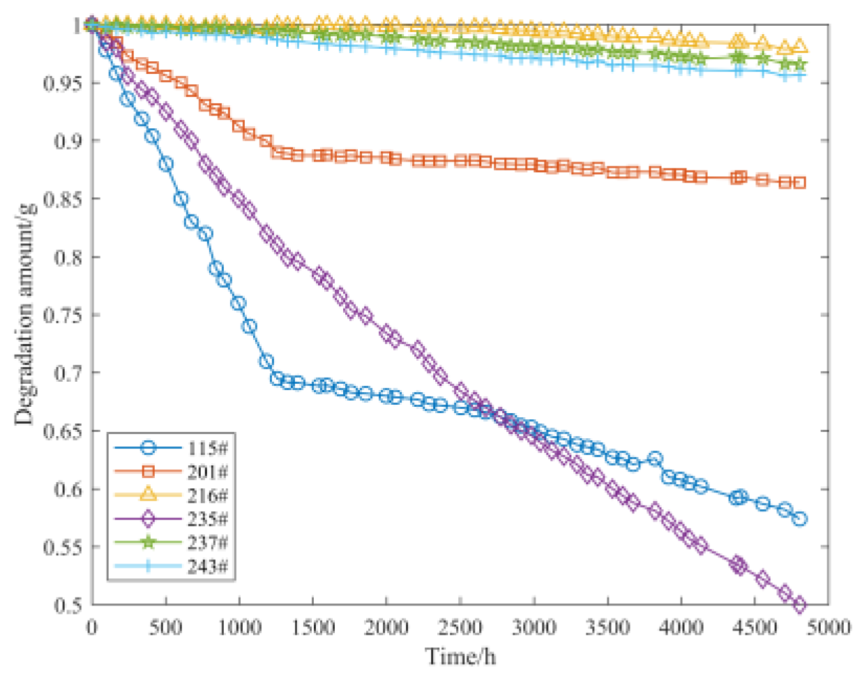
4.1. Data Description

This section utilizes the SDSADT data from a specific missile tank to verify the effectiveness and feasibility of the SDRD method. The tank is the cooling device for a missile seeker, which has the characteristics of high-reliability and long-life. It contains a certain amount of freon, which will continuously leak due to the influence of temperature during storage in the warehouse. When the leakage amount reaches the failure threshold, the cooling effect of the tank makes it difficult to meet the requirements of the missile seeker, at which point the tank is judged to have failed. Under normal stress levels, the leakage process of freon is very slow. High temperatures can accelerate the leakage of freon; therefore, it is necessary to carry out temperature stress ADT to evaluate its storage life. Reference [22] assessed the storage life of the tank based on the cumulative damage theory and provided detailed test plans and test data. This article selects the same test data as in Reference [22] to verify the effectiveness and feasibility of the proposed method. The specific details of the SDSADT for the specific missile tank are shown in

Table 1. Specific details of the SDSADT for a specific missile tank.

No.	Test Parameter	Specific Details
1	Sample size	$n=6$
2	The number of stress levels	$k=3$
3	Stress levels/K 1	$S_3=333$$,S_2=323$$,S_1=318$
4	Normal stress level/K 1	$S_0=298$
5	Detection number	$m_3=15$$,m_2=15$$,m_1=23$
6	Stress transition moment/h	$t_1=1258$$,t_2=2672$$,t_3=4802$
7	Failure threshold/g 2	$D_f=1.2$
8	Test period/h	About 72
9	Index storage life/h 3	43,800

¹ In this article, the unit for stress levels used in formula derivation and calculation is Kelvin, so the unit in Table 1 is unified as Kelvin (K). ² Refer to Reference [22] to determine the quality of the freon leakage of the missile tank in the unit g. ³ The index storage life represents the specified storage life of the product at the time of manufacture and shipment. In this case, the index storage life for the missile tank is 5 years, which is equivalent to 43,800 h.

.

In the test, the freon leakage amount of the missile tank is selected as its performance parameter. When the leakage amount exceeds the set value of 1.2 g, the tank is considered to have failed. The missile tank has an indicator storage life of 5 years under normal stress levels, which equates to 43,800 h. The degradation curve of the missile tank under the SDSADT is shown in Figure 3. From the figure, it is evident that the degradation paths of the six products in the SDSADT exhibit significant randomness. Therefore, it is meaningful to introduce the Gamma distribution to characterize the randomness of the product degradation paths in this article.

4.2. Comparison Method

To verify the effectiveness and feasibility of the SDRD method, it is compared with several advanced methods.

(1)

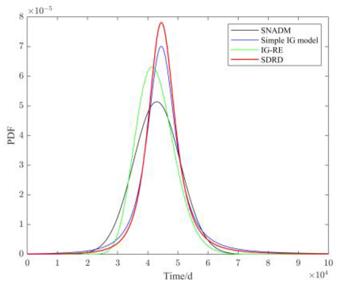
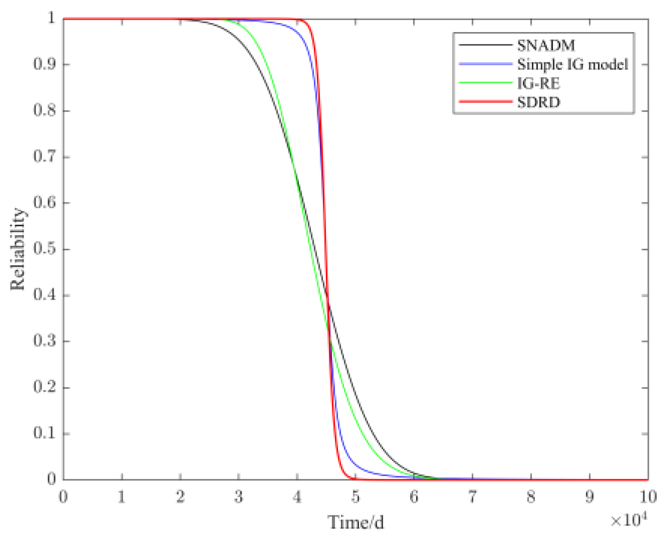
SNADM: This method is based on an equivalent approach of the cumulative damage theory to derive the piecewise expression for the overall cumulative degradation function. It then combines the nonlinear function to obtain a Segmented Nonlinear Accelerated Degradation Model (SNADM). Subsequently, numerical iterative methods are used to estimate the model parameters [22].

(2)

Simple IG process: This method uses an IG process-based approach described in Section 2.2 of this article, which ignores the randomness of the degradation paths among different samples. It assumes that all samples share the same performance degradation process and uses the MLE method to estimate the model parameters.

(3)

IG model considering random effects (IG-RE): This method only considers the randomness of the product degradation paths and uses the Markov Chain Monte Carlo (MCMC) method to estimate the unknown parameters in the degradation model [21].

4.3. Parameter Estimation and Result Analysis

Based on the SDSADT data for the specific missile tank, the parameters in Equation (24) are estimated using the MC method. The estimated values for the parameters are ${\widehat{\alpha }}_0=-10.5291$, ${\widehat{\alpha }}_1=0.7985$, $\widehat{\delta }=3.2602$, $\widehat{\gamma }=3.395\times {10}^{-6}$, and ${\widehat{\sigma }}_{\epsilon }^2=0.1226$. By substituting the above parameter values into Equation (26), the storage life of the missile tank under normal stress levels can be obtained. In addition, the relationship function between product degradation path and stress level can be obtained by substituting the parameter estimates ${\widehat{\alpha }}_0=-10.5291$ and ${\widehat{\alpha }}_1=0.7985$ into Formula (3), as shown in Figure 4. As can be seen from the figure, the higher the stress level applied, the more obvious the product degradation path. Generally, the missile tank is considered to have failed when its reliability is below 0.9. From Equation (26), it is evident that when the reliability of the product under normal stress is 0.9, the storage time of the product is 43,401 h. Therefore, the average storage life of the missile tank based on the SDRD method is 43,401 h.

Compared with the method proposed in this article, the parameter estimates of the SNADM model are ${\widehat{\alpha }}_0=1.1025$, $\widehat{a}=21.6517$, and $\widehat{b}=9897.7$. By substituting the parameter values into the reliability function, the storage life of the product under normal stress conditions can be calculated as 42,291 h. The parameter estimates of the simple IG model are ${\widehat{\alpha }}_0=-10.4705$, ${\widehat{\alpha }}_1=-1.2701$, and $\widehat{\lambda }=1.9431\times {10}^{-8}$. By substituting the parameter values into the reliability function of Equation (9), the storage life of the product under normal stress conditions can be calculated as 43,028 h. The parameter estimates of the IG process model considering random effects are ${\widehat{\alpha }}_0=-4.7091$, ${\widehat{\alpha }}_1=0.3864$, $\widehat{\delta }=8.2703\times {10}^{-6}$, and $\widehat{\gamma }=3.7615\times {10}^{-7}$. By substituting the parameter values into the reliability function, the storage life of the product under normal stress can be calculated as 43,359 h.

The storage life values of the missile tank calculated by each method are shown in

Table 2. The average storage life of a certain type of missile tank.

Models	Index Storage Life/h	Storage Life Assessment Value/h
SNADM 1	43,800	42,291
Simple IG model 2		43,028
IG-RE 3		43,359
SDRD 4		43,401

¹ SNADM refers to the Segmental Nonlinear Accelerated Degradation Model proposed in Reference [18]. ² The simple Inverse Gaussian (IG) model is the method for life assessment based on the IG process in Section 2.2 of this article. ³ IG-RE refers to the IG process model considering random effects proposed in Reference [21]. ⁴ SDRD refers to the step-down stress accelerated degradation test assessment method which considers random effects and detection errors.

. As shown in Table 2, the storage life assessment methods based on the SNADM and the simple IG process model do not consider the impact of random factors between different samples and the impact of uncertain factors such as detection environment and detection equipment. Therefore, their life assessment results are not satisfactory. The IG process model that considers random effects does take into account the randomness of and difference in product degradation paths. However, it still cannot avoid the impact of detection errors. Therefore, the effectiveness of this model in life assessment is second only to the SDRD model. The storage life assessment results indicate that the proposed SDRD model performs well in assessing the storage life of high-reliability and long-life products, and the assessment value is close to the index storage life. This is primarily due to the following reasons: First, the Gamma distribution is introduced to characterize the randomness among the degradation paths of different products. This approach enhances the life assessment capability of the IG performance degradation model. Second, considering the impact of detection errors on product degradation, the normal distribution is used to describe the detection errors of performance parameters. In addition, the MC method is used to replace traditional parameter estimation methods for estimating model parameters. This method can enhance calculation accuracy and efficiency. Therefore, the proposed SDRD model is more effective for assessing the storage life of high-reliability, long-life products.

Based on the PDF and reliability models of each method, their PDF graphs and reliability function curves can be obtained, as shown in Figure 5 and Figure 6. From Figure 5, it can be seen that the peak of the proposed SDRD method is higher and the range of variation is narrower. This indicates that the data distribution is more concentrated and the accuracy of its life assessment is higher. From Figure 6, it is very clear that compared to other methods, the SDRD method has a better performance in storage life assessment. However, the reliability function curves of the storage life assessment methods based on the SNADM and simple IG process models do not show significant differences. Therefore, the Akaike Information Criterion (AIC) and Bayesian Information Criterion (BIC) are used to select the model quantitatively. Compared with the AIC, the BIC has a greater penalty for model complexity. To prevent overfitting, the BIC tends to choose models with fewer parameters. In contrast, the AIC imposes a relatively smaller penalty for complexity when selecting models. To enhance the life assessment ability of the model, AIC tends to favor models with more parameters. Based on this, this article has calculated the AIC and BIC values for four methods: SNADM, simple IG model, IG-RE, and SDRD. The formulas for the AIC and BIC are as follows:

$$AIC=-2\times \ln L\left(\widehat{\mathit{\theta }}\right)+2\varpi$$

(27)

$$BIC=-2\times \ln L\left(\widehat{\mathit{\theta }}\right)+\varpi \ln \left(n\right)$$

(28)

where $\ln L\left(\widehat{\mathit{\theta }}\right)$ is the estimate of the log-likelihood function. $\varpi$ is the number of parameters. $n$ is the number of samples.

Based on Formulas (27) and (28), the AIC values and the BIC values for each model are calculated and shown in

Table 3. AIC and BIC results of each model.

Models	SNADM	Simple IG Model	IG-RE	SDRD
AIC	−10.15	−32.23	−60.89	−72.28
BIC	−10.77	−32.85	−61.72	−73.32

. It can be seen from the table that the AIC and the BIC of the proposed SDRD model are the smallest. This indicates that the SDRD model has a better fitting effect on the data and reduces the risk of overfitting. It further prevents the issue of excessively high model complexity due to overly high model precision and avoids the phenomenon of the curse of dimensionality. Therefore, the SDSADT assessment method proposed in this article, which considers random effects and detection errors, is more accurate and reasonable.

5. Conclusions

This article proposes the SDSADT assessment method, which takes into account random effects and detection errors (SDRD). This method can solve the problem of slow performance degradation rates at the early stages of the step-stress ADT and enhance the efficiency of the accelerated test. Considering the randomness of product degradation paths, the Gamma distribution is introduced and the normal distribution is used to describe the detection errors of performance parameters. In addition, the unknown parameters in the IG performance degradation model are estimated using the MC method. By comparing the proposed method with currently advanced methods, the results show that the storage life assessment value of the SDRD model is close to the index storage life, and the storage life assessment performance is better. Therefore, the SDRD model is more effective for assessing the storage life of high-reliability and long-life products. However, there may be multiple performance parameters in the actual ADT for other high-reliability, long-life products such as fuse springs. If only a single performance parameter is considered, the reliability assessment results may be inaccurate due to insufficient degradation data. Therefore, it is necessary to establish corresponding reliability models based on the data characteristics of each performance parameter. This topic can be explored in future research.

References

1. Chen, Y.; Zhang, Q.; Cai, Z.; Wang, L. Storage Reliability Assessment Model Based on Competition Failure of Multi-Components in Missile. J. Syst. Eng. Electron. 2017, 28, 606–616. [Google Scholar]
2. Wang, X.; Wang, B.; Wu, W.; Hong, Y. Reliability Analysis for Accelerated Degradation Data Based on the Wiener Process with Random Effects. Qual. Reliab. Eng. 2020, 36, 1969–1981. [Google Scholar] [CrossRef]
3. Jiang, P.; Wang, B.; Wang, X.; Zhou, Z. Inverse Gaussian Process Based Reliability Analysis for Constant-Stress Accelerated Degradation Data. Appl. Math. Model. 2022, 105, 137–148. [Google Scholar] [CrossRef]
4. Feng, X.; Tang, J.; Tan, Q.; Yin, Z. Reliability Model for Dual Constant-Stress Accelerated Life Test with Weibull Distribution under Type-I Censoring Scheme. Commun. Stat. Theory Methods 2022, 51, 8579–8597. [Google Scholar] [CrossRef]
5. Lim, H.; Yum, B. Optimal Design of Accelerated Degradation Tests Based on Wiener Process Models. J. Appl. Stat. 2011, 38, 309–325. [Google Scholar] [CrossRef]
6. Wang, L.; Pan, R.; Li, X.; Jiang, T.A. Bayesian Reliability Evaluation Method with Integrated Accelerated Degradation Testing and Field Information. Reliab. Eng. Syst. Saf. 2013, 112, 38–47. [Google Scholar] [CrossRef]
7. Méndez-González, L.; Rodríguez-Picón, L.; Pérez Olguin, I.; Garcia, V.; Quezada-Carreón, A. Reliability Analysis for DC Motors under Voltage Step-Stress Scenario. Electr. Eng. 2020, 102, 1433–1440. [Google Scholar] [CrossRef]
8. Tang, S.; Guo, X.; Yu, C.; Xue, H.; Zhou, Z. Accelerated Degradation Tests Modeling Based on the Nonlinear Wiener Process with Random Effects. Math. Probl. Eng. 2014, 2014, 1–11. [Google Scholar] [CrossRef]
9. Sun, L.; Gu, X.; Song, P. Accelerated Degradation Process Analysis Based on the Nonlinear Wiener Process with Covariates and Random Effects. Math. Probl. Eng. 2016, 2016, 1–13. [Google Scholar] [CrossRef]
10. Wang, H.; Zhao, Y.; Ma, X. Mechanism Equivalence in Designing Optimum Step-Stress Accelerated Degradation Test Plan under Wiener Process. IEEE Access 2018, 6, 4440–4451. [Google Scholar] [CrossRef]
11. Zhang, C.; Chen, X.; Wen, X. Step-Down-Stress Accelerated Life Test-Methodology. Acta Armamentarii 2005, 26, 661–665. [Google Scholar]
12. Cai, M.; Yang, D.; Zheng, J.; Mo, Y.; Huang, J.; Xu, J.; Chen, W.; Zhang, G.; Chen, X. Thermal Degradation Kinetics of LED Lamps in Step-Up-Stress and Step-Down-Stress Accelerated Degradation Testing. Appl. Therm. Eng. Des. Process. Equip. Econ. 2016, 107, 918–926. [Google Scholar] [CrossRef]
13. Qi, H.; Zhang, X.; Xie, X.; Lv, C.; Chen, C.; Zhao, L. Storage Life of Power Switching Transistors Based on Performance Degradation Data. J. Semicond. 2014, 35, 044006. [Google Scholar] [CrossRef]
14. Hong, Y.; Duan, Y.; Meeker, W.; Stanley, D.; Gu, X. Statistical Methods for Degradation Data with Dynamic Covariates Information and an Application to Outdoor Weathering Data. Technometrics 2015, 57, 180–193. [Google Scholar] [CrossRef]
15. Liu, T.; Sun, Q.; Pan, Z.; Feng, J.; Tang, Y. Irregular Time-Varying Stress Degradation Path Modeling: A Case Study on Lithium-ion Cell Degradation. Qual. Reliab. Eng. Int. 2016, 32, 1889–1902. [Google Scholar] [CrossRef]
16. Tang, J.; Su, T.S. Estimating Failure Time Distribution and Its Parameters Based on Intermediate Data from a Wiener Degradation Model. Nav. Res. Logist. 2008, 55, 265–276. [Google Scholar] [CrossRef]
17. Wang, X.; Xu, W. An Inverse Gaussian Process Model for Degradation Data. Technometrics 2010, 52, 188–197. [Google Scholar] [CrossRef]
18. Zhang, S.; Zhou, W.; Qin, H. Inverse Gaussian Process-Based Corrosion Growth Model for Energy Pipelines Considering the Sizing Error in Inspection Data. Corros. Sci. 2013, 73, 309–320. [Google Scholar] [CrossRef]
19. Peng, W.; Li, Y.; Yang, Y.; Huang, H.; Zuo, M. Inverse Gaussian Process Models for Degradation Analysis: A Bayesian Perspective. Reliab. Eng. Syst. Saf. 2014, 130, 175–189. [Google Scholar] [CrossRef]
20. Tsai, T.; Sung, W.; Lio, Y.; Chang, S.; Lu, J. Optimal Two-Variable Accelerated Degradation Test Plan for Gamma Degradation Processes. IEEE Trans. Reliab. 2016, 65, 459–468. [Google Scholar] [CrossRef]
21. Kou, H.; Wei, K. The Evaluation Method for Step-Down-Stress Accelerated Degradation Testing Based on Inverse Gaussian Process. IEEE Access 2021, 9, 73194–73200. [Google Scholar]
22. Yao, J.; Xu, M.; Zhong, W. Research of Step-Down Stress Accelerated Degradation Data Assessment Method of a Certain Type of Missile Tank. Chin. J. Aeronaut. 2012, 25, 917–924. [Google Scholar] [CrossRef]
23. Gao, L.; Chen, W.; Qian, P.; Pan, J.; He, Q. Optimal Design of Multiple Stresses Accelerated Life Test Plan Based on Transforming the Multiple Stresses to Single Stress. Chin. J. Mech. Eng. 2014, 27, 309–325. [Google Scholar] [CrossRef]
24. Smith, A.; Roberts, G. Bayesian Computation via the Gibbs Sampler and Related Markov Chain Monte Carlo Methods. J. R. Stat. Soc. Ser. B (Methodol.) 1993, 55, 3–23. [Google Scholar] [CrossRef]
25. Lee, Y.; Lu, M. Damage-Based Models for Step-Stress Accelerated Life Testing. J. Test. Eval. 2012, 34, 1–10. [Google Scholar] [CrossRef]
26. Peng, C.Y. Inverse Gaussian Processes with Random Effects and Explanatory Variables for Degradation Data. Technometrics 2015, 57, 100–111. [Google Scholar] [CrossRef]
Figure 1. The SDSADT stress profile diagram.
Applsci 14 07209 g001
Figure 2. The flowchart for parameter estimation and life assessment based on the MC method.
Applsci 14 07209 g002
Figure 3. Degradation path curve of the missile tank under the SDSADT.
Applsci 14 07209 g003
Figure 4. The functional relationship between stress level and product performance degradation.
Applsci 14 07209 g004
Figure 5. The PDF graphs for each model.
Applsci 14 07209 g005
Figure 6. The reliability function curves for each model.
Applsci 14 07209 g006