Article

Research on the Jiamusi Area’s Shallow Groundwater Recharge Using Remote Sensing and the SWAT Model

1
School of Hydraulic and Electric Power, Heilongjiang University, Harbin 150080, China
2
Institute of Groundwater Cold Region, Heilongjiang University, Harbin 150080, China
3
International Joint Laboratory of Hydrology and Hydraulic Engineering in Cold Regions of Heilongjiang Province, Harbin 150080, China
*
Author to whom correspondence should be addressed.
Appl. Sci. 2024, 14(16), 7220; https://doi.org/10.3390/app14167220
Submission received: 8 July 2024 / Revised: 18 July 2024 / Accepted: 13 August 2024 / Published: 16 August 2024
(This article belongs to the Special Issue Sustainable Environment and Water Resource Management)

Abstract

:
Jiamusi is situated in Heilongjiang Province, China, in the center of the Sanjiang Plain. The 1980s’ overplanting of paddy fields resulted in a decrease in groundwater levels, scarcity of groundwater resources, and frequent earth collapses. Examining and safeguarding the groundwater resources in this region has emerged as a crucial subject. In light of this, this paper uses the remote sensing water balance method and the SWAT distributed hydrological model to calculate groundwater resources in the Jiamusi area. It also conducts scientific experiments by examining various factors, including rainfall, the degree of water supply, soil type, and land use. The measured monthly runoff of Jiamusi City’s Tongjiang and Fuyuan City’s hydrology stations was utilized to establish the model parameters for the SWAT model. A preliminary assessment of the distribution features of shallow groundwater in the Jiamusi area is conducted using the two methodologies mentioned above, and the following results are reached: (1) Tongjiang Hydrological Station and Fuyuan Hydrological Station both had good runoff modeling results, with R2 and NS values of 0.81, 0.77, and 0.77, 0.75, respectively. (2) The SWAT model works well for assessing groundwater resources. Between 2010 and 2016 (two preheating years), Jiamusi’s average groundwater recharge was 61.03 × 10⁸ m3, with a recoverable amount of 27.4 × 10⁸ m3. (3) Based on the remote sensing water balancing approach, the average exploitable quantity of groundwater recharge in the Jiamusi area between 2008 and 2016 is 23.94 × 10⁸ m3, while the average recharge in the area is 53.2 × 10⁸ m3. (4) The Jiamusi metropolitan area is the core of the groundwater phreatic reservoir water reserves, which progressively decline in both the northeast and southeast directions. It falls to the southwest as Fuyuan City’s center. The Songhua River’s main stream area near Tongjiang City has the least volume of water reserves in the phreatic layer, and the area’s groundwater reserves converge to the southeast and northwest, where surface water makes up the majority of the water resources.

1. Introduction

Jiamusi lies on the alluvial plain where the Songhua, Heilongjiang, and Ussuri rivers converge in northeast China. It is an important ecological functional area of the country and a grain-producing area [1]. The Jiamusi region’s unique geographical location indirectly causes heavy soil texture and low drainage capacity, which is prone to waterlogging disasters and yield reductions [1]. As a result, since the 1980s, the amount of rice planting and drilling in Jiamusi has surged [2]. In 2020, about 80% of the growing area in the region was paddy fields [3]. These technologies improve soil texture, control drainage capacity, and help prevent flooding, but they also make groundwater resources more scarce and even cause serious ecological problems such as ground collapse and groundwater level decline in some places [4]. The groundwater level of Jiamusi City needs to be repaired immediately [5]. The calculation and evaluation of groundwater resources form the data support and premise for putting forward the restoration plan, so this paper evaluates the groundwater resources in the Jiamusi area under this background.
In recent years, there have been a lot of studies on groundwater resources at home and abroad. Demlie [6] used the soil water balance and chloride ion mass balance methods to estimate groundwater recharge in Ethiopia’s Akaki Basin. Based on the study results, Demlie said the maximum recharge value of the basin can be represented by the average recharge value determined by the soil water balance method and the chloride ion mass balance method. In addition, Hornero [7] used the same method to estimate the recharge of the Alcadozo aquifer system in Spain and conducted an uncertainty analysis of the results of both methods. Delin et al. evaluated groundwater recharge in Minnesota using the unsaturated zone water balance, groundwater dating, groundwater table fluctuation methods, and regional regression recharge model (RRR). They then compared and evaluated the charges obtained using the different methods. Zhang et al. combined the soil water balance model with the groundwater table fluctuation method to strengthen and verify the evaluation results of groundwater recharge in the upper Danube basin. Yin Lihe et al. [8] selected groundwater recharge evaluation methods, such as the water balance, saturation zone Darcy’s law, and groundwater level fluctuation methods, according to the actual situation of the study area and estimated the average annual groundwater recharge rate in Ordos Plain, Inner Mongolia. Although a large number of studies have produced a large number of results, they have all been derived using traditional formulas. Because the field investigation is time-consuming and laborious, and the problems, such as a lack of monitoring points in the steep and changeable terrain, are difficult to solve, the evaluation results are relatively biased. Therefore, this study selected Jiamusi City as the research object [9] and used the SWAT model and remote sensing water balance method to simulate groundwater resources in this area [10,11]. Compared with traditional methods, the remote sensing water balance method has the advantage of integrating a global road surface data assimilation system and RSGIS and provides faster and more convenient data retrieval. These technologies are also the focus areas of current research and the future development direction [12]. In addition, the large coverage area and small temporal resolution of remote sensing significantly reduce the influence of the rainfall infiltration coefficient method on geological water storage and runoff, which are often neglected factors [13], and improve the accuracy of groundwater resource calculation. In addition, in order to improve the accuracy of the research results, the SWAT model was also adopted in this study. On the basis of identifying the sensitive factors, the model uses the hydrological response units divided by the model to maintain the regional consistency of climate, soil, and land use and verify the applicability of the model. Subsequently, the shallow groundwater resources in the whole study area were evaluated. This study has important reference values for the restoration of groundwater levels and agricultural and grain production in the Sanjiang Plain.

2. Overview of the Study Area

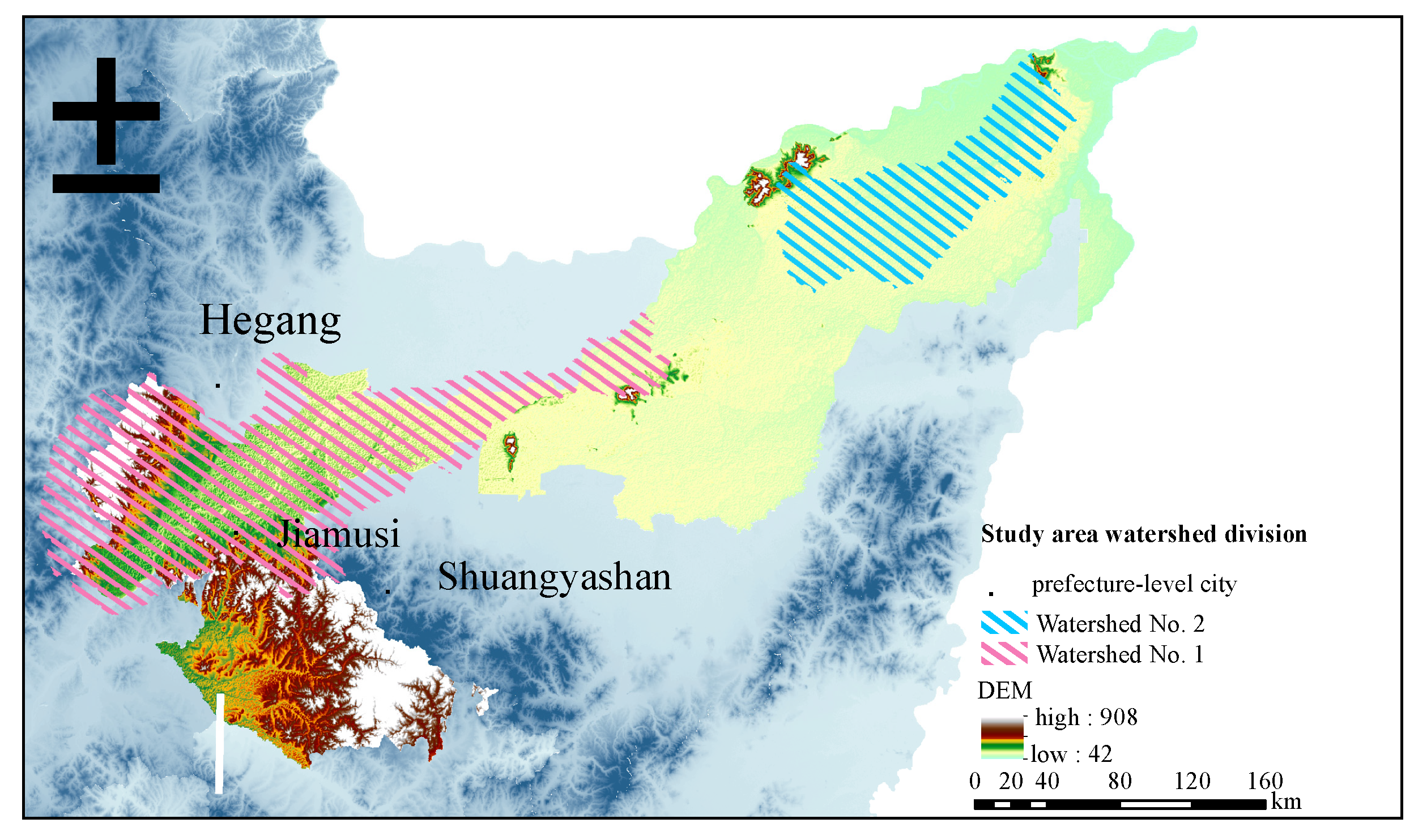
Jiamusi City is located in the hinterland of the Sanjiang Plain, which is formed by the confluence of the Songhua River, Heilongjiang River, and Ussuri River at the northeast border of China [14]. It faces Heilongjiang in the northeast, Russia in the east, and Raohe County and Fuyuan City in the east. Yilan and Boli Counties border the southwest border. It is adjacent to Qitaihe City and Shuangyashan City. Yichun City is connected with the northwest border. The city of Hegang is to the north [15]. The area is 388 km long from east to west and 150 km wide from north to south, both long and narrow. There are more than 130 large and small rivers in the area, and the main water systems are the Heilongjiang, Songhua, and Wusuli Rivers. These rivers are the Songhua River, the Black Dragon River, and the first and second tributaries of the Wusuli River, distributed in the county (city) of Jiamusi City. Its terrain slopes roughly from southwest to northeast, with the highest point in the southwest and the lowest point in the northeast. This area is mainly composed of three different types of landforms: accumulation plain, erosion accumulation front, erosion denudation low hills and hills [16]. Due to its complex geological structure, many factors affect the groundwater level, mainly the lateral replenishment of atmospheric precipitation and the Tongjiang–Fuyuan section of the Heilongjiang and the Jiamusi–Tongjiang section of the Songhua River. The average annual precipitation in this area is 540 mm, and atmospheric precipitation is the main source of groundwater recharge. The distribution of precipitation is uneven within the year, and the precipitation in July, August, and September accounts for about 59.5% of the annual precipitation, which is the main recharge period for groundwater. In addition, the groundwater extraction in Jiamusi area is large. According to the introduction of Yu Haijiang, director of the Jiamusi Water Bureau, the well irrigation area of the Jiamusi area reaches 5 million mu, accounting for more than 73.5% of the actual irrigation area of the whole area. According to the average annual water consumption of 750 cubic meters per mu, the annual demand for groundwater resources in the well irrigation area is 3.75 billion cubic meters, while the average annual groundwater resources are 3.307 billion cubic meters, and the groundwater over-extraction is more than 443 million cubic meters. A summary is shown in Figure 1 and Figure 2. Two basins were divided using the SWAT model, which served as the basis for subsequent simulation studies.

3. Materials and Methods

3.1. Sources of Data

3.1.1. Data on Elevation

According to certain research, the elevation map with a resolution of 20–150 m should be chosen when using SWAT to model runoff [17]. The digital elevation map (DEM) and elevation data, which were downloaded from the NASA Earth Science Data website at a resolution of 30 m, were utilized in this work to extract pertinent watershed metrics.

3.1.2. Data on Soil Type

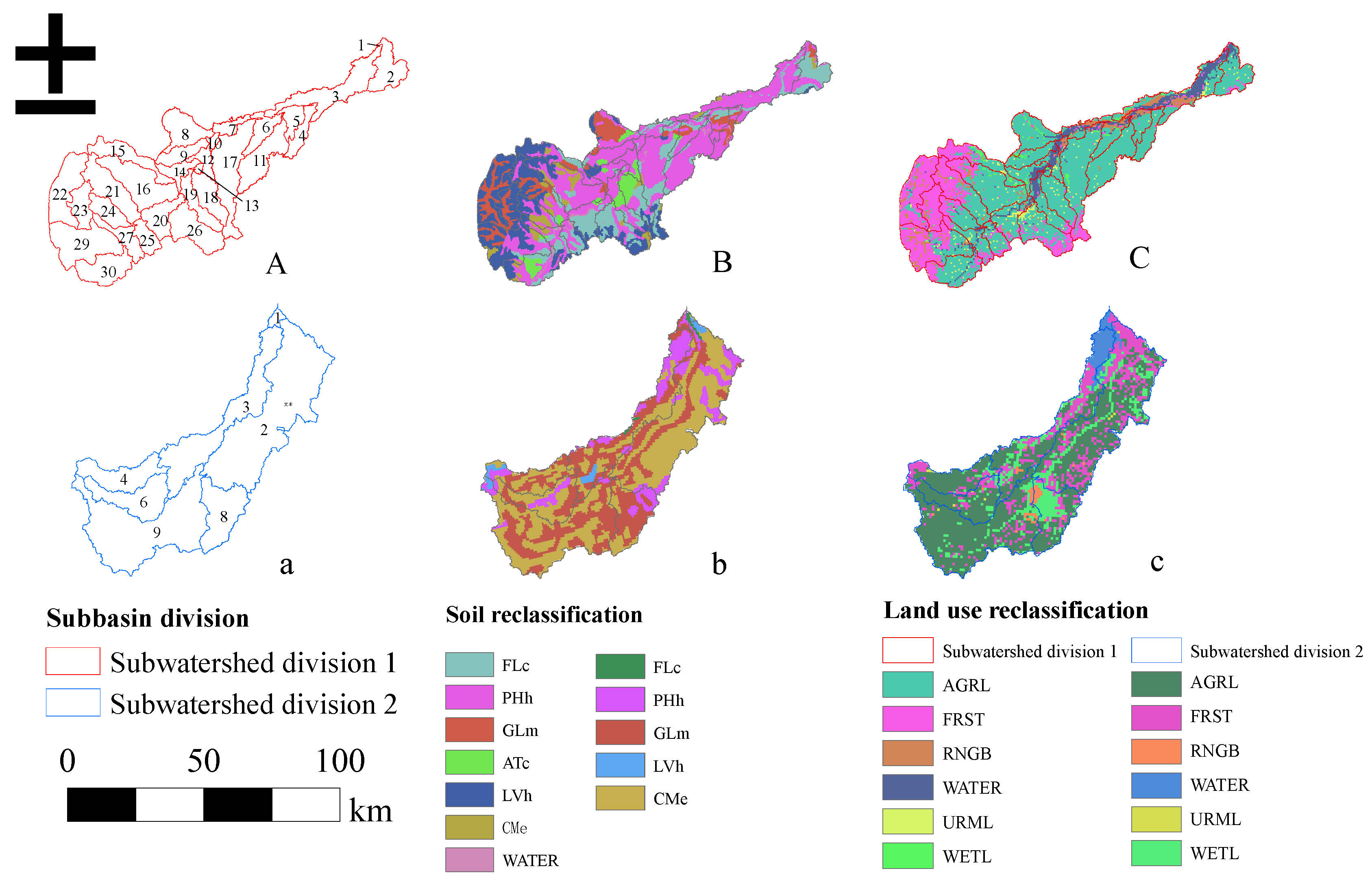
The physical characteristics and spatial distribution of various soil types in the study area are listed in the soil database. The 1:100,000 soil data used in this paper had a resolution of 1000 km2. According to the physical characteristics of the soil, the soil types of the two drainage basins were classified, and drainage basin No. 1 was divided into 6 soil groups, in which PHh soil accounted for 25.23% of the highest proportion, and Cme soil accounted for 0.35% of the lowest proportion. There are 5 different soil types in the No. 2 drainage basin, among which PHh is the highest (28.98%), and CMe is the lowest (0.44%). Compared with the soil type of the No. 1 watershed, the No. 2 watershed has no ATc soil type. See Table 1 below for details.
In this study, in order to calculate the soil data parameters of the SWAT model, it is necessary to convert the amount of carbon deposited in the soil layer into organic matter and then input the result into SPAW software (6.02.75 version) for calculation. The database also includes the amount of clay, clay loam, and gravel in the soil. In order to facilitate the calculation of USLE-K parameters in the model, Williams’s alternative [18] formula: R = n j = 1 ( 1.213 + 0.89 l o g 10 I j ) ( I j T j ) 173.6 × I 30 I j 1 T j 30 1 was adopted. Table 2 and Table 3 give the exact values for layers 1 and 2 of the final calculation results. In the calculation, the description of the correlation coefficient of each level of soil involved can be referred to in Table 4.

3.1.3. Type Data of Land Use

The land use data originate from the Chinese Academy of Sciences’ Academy of Aerospace Information Innovation’s 2022 global 30 m resolution land cover. Six categories were created from the reclassification of the land use types in the No. 1 and No. 2 watersheds (see Figure 3). These categories included cultivated land, forest land, grassland, water area, urban and rural areas, industrial and mining land, residential property, and unused land. Table 5 displays the related categories of model inputs.

3.1.4. Info about the Weather and Runoff

The observed meteorological data were entered into the SAWT model in the first stage, and the weather generator was then constructed based on the input model, which comprised the meteorological database component of the SWAT model. The primary daily meteorological data that were used were those related to temperature, relative humidity, solar radiation, wind speed, and precipitation. The National Tibetan Plateau Scientific Data Center provided the CMADSV1.1 meteorological data that were used in this work [19]. The time length was from 2008 to 2016, the spatial resolution was 0.25, and the time resolution was day by day. These parameters essentially satisfied the requirements of the experimental time scale. One of the most popular databases for SWAT model meteorological data is this one, and if the measured meteorological data are modified, the simulation accuracy will increase dramatically. The precipitation temperature, relative humidity, sun radiation, wind speed, and 60 meteorological stations in the study area were chosen as experimental meteorological data in this work based on the Jiamusi DEM data range. From 2008 to 2016, monthly runoff data from the Fuyuan Hydrology Station, which is located at the complete outlet of the No. 2 watershed, and the Tongjiang Hydrology Station, which is located at the total outlet of the No. 1 watershed, were chosen.

3.1.5. Data for the Water Balance Technique Using Remote Sensing

The Jiamusi hydrology station provided the majority of the data used in this computation approach. Among them were the precipitation, evapotranspiration, and regional average runoff depth, which were collected using TRMM [20] data, MOD16 software (MOD16A2GF V061 version) [21] synthesis, and GLADS-2.1 (Global Land Data Assimilation System) [22] model estimation, respectively, and used to compute groundwater recharge in the research area by remote sensing technology.
To sum up, details of all data studied in this paper are shown in Table 6.

3.2. Research Methods

3.2.1. Remote Sensing Water Balance Method

Groundwater recharge is defined as the difference between rainfall and evapotranspiration and runoff when employing the remote sensing water balance method. The following Formula (1) [23,24] was used to calculate groundwater recharge:
R = P S E T Δ S
where R is the groundwater recharge amount (mm); Rainfall (mm); S is the annual average runoff (mm); ET is the evapotranspiration (mm); Δ S is the store changes (mm) for soil water. Details of the method can be found in reference [25].

3.2.2. SWAT Model

The SWAT model (Soil and Water Assessment Tool) is a basin-scale semi-distributed hydrological model developed by the Agricultural Research Service (ARS) of the United States Department of Agriculture (USDA) with daily time steps. It mainly includes the hydrologic process, soil erosion, and pollution load sub-models. SWAT models can simulate surface water, soil water, and groundwater processes. The data can also be subdivided into multiple natural sub-basins based on the real topography of the basin, effectively reducing the impact of the spatiotemporal variation in natural factors on the simulation results and further dividing corresponding hydrological units within the scope of the sub-basin for collaborative change feature simulation [26].
Equation (2) displays the water balance formula based on the hydrological cycle process simulation of the SWAT model.
S W t = S W 0 + i = 1 t ( R d a y , i Q s u r f , i E a , i W s e e p , i Q g w , i )
where S W t is the soil water content at the end of the period, mm; S W 0 is the soil water content at the beginning of the period, mm; t is the calculation period; R d a y , i is the rainfall of day i, mm; S s u r f , i is the surface runoff of day i, mm; E a , i is the evaporation amount of day i, mm; W s e e p , i is the permeability of day i, mm; Q g w is the underground runoff on day i, mm.

3.2.3. Shallow Aquifer Reservoir Variable Calculation Method

Based on the calculation principle of groundwater balance, the calculation formula for shallow aquifer reservoir variables is as follows:
S g w = P E R C G W Q R E V A P D A R C
where Δ S g w is the shallow aquifer reservoir variable (mm); P E R C is the leakage water of the vadose zone (mm); R E V A P is the water quantity of aquifer regression vadage zone (mm); D A R C is the seepage volume of a deep aquifer (mm); G W Q is the contribution of underground runoff to the main river course (mm).
The groundwater runoff modulus method was used to calculate the natural supply of the basin, and the specific formula is as follows:
Q = M · F · t · 10 7
where Q is the natural supply amount (10,000 m3); M is the groundwater runoff modulus (L/(s·km2)); F is the catchment area (km2); t is time (s). The groundwater runoff modulus was calculated as follows:
M y e a r = W y e a r F × t × 1000
where W y e a r is the average under-land runoff in time step (m3); F is the catchment area (km2); t for time (s)
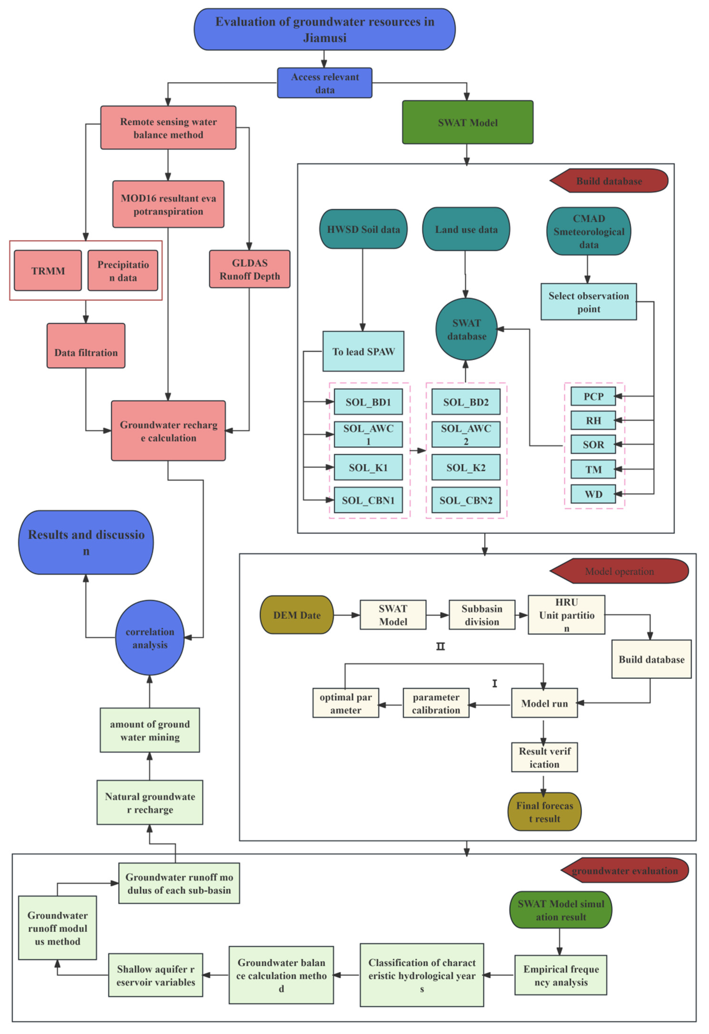
The data and research techniques used in this work are listed above. Two methods were used in this paper. First, groundwater recharge estimation and recoverable amount calculation were carried out using the remote sensing water balance method. The precipitation data are TRMM data after comparison with the rain measuring station. The evapotranspiration data were synthesized by mod16, and the net flow depth data were simulated and synthesized by GLADS-2.1 software and finally brought into the formula to obtain the results. Using the SWAT model for the laboratory, first, the HWSD soil database, CMADS meteorological database, and land use data were imported into the SWAT model for database construction. SPAW software (6.02.75 version) was used to calculate soil level in the construction of the soil type database. After running the model, parameter calibration was carried out, and the range of selected parameters was continuously reduced to adjust parameters, and finally, the optimal parameters were obtained. Then, the simulated results were substituted into the groundwater water balance and the groundwater runoff modulus calculation equations, and the groundwater runoff modulus and groundwater recharge were obtained, respectively. Then, the obtained results were compared with those obtained by the remote sensing water balance method, and the groundwater resources in the study area were comprehensively evaluated. The details are shown in Figure 4 below:

4. Results

4.1. From 2008 to 2016, Jiamusi’s Groundwater Recharge Was Calculated Using the Remote Sensing Water Balance Method

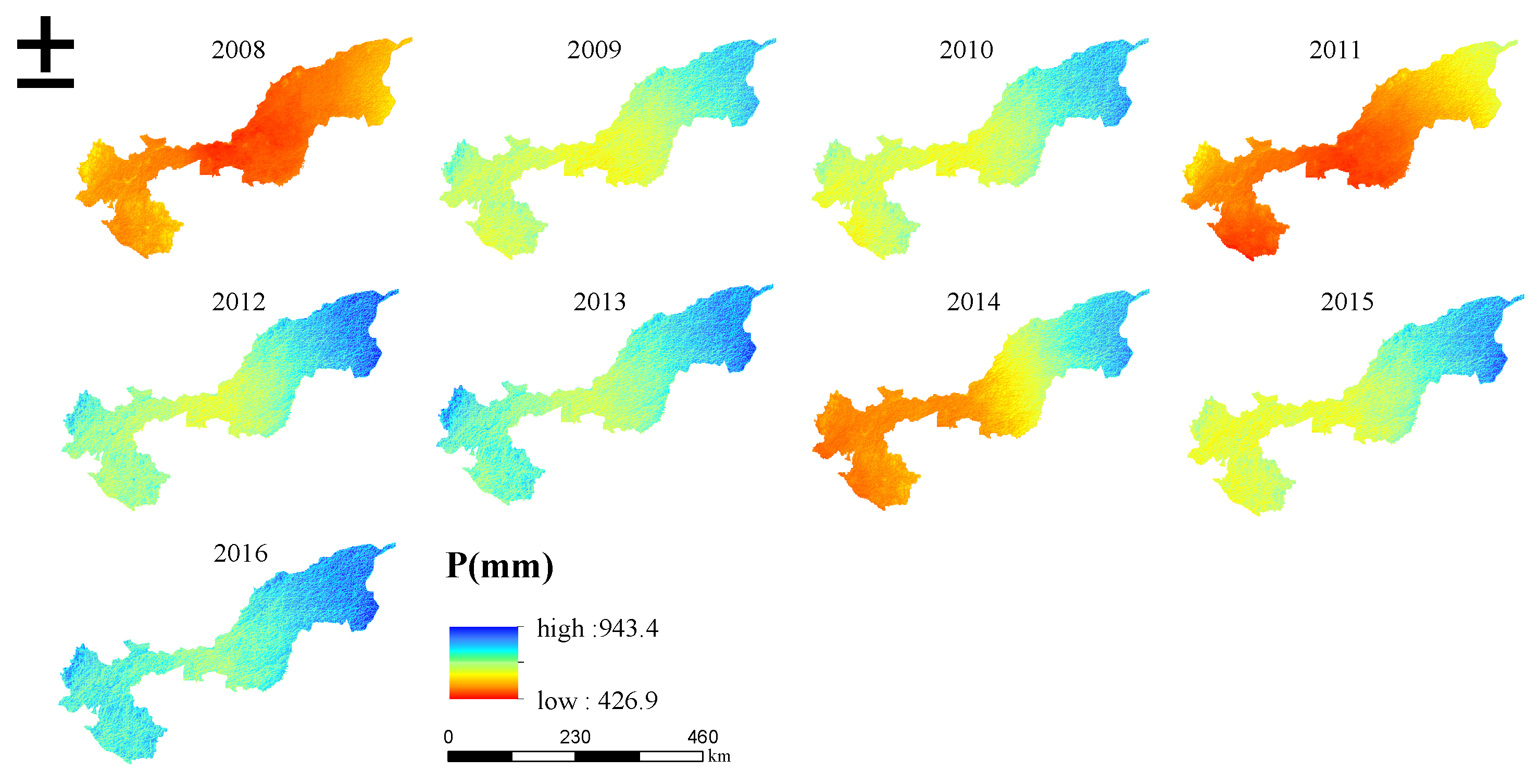
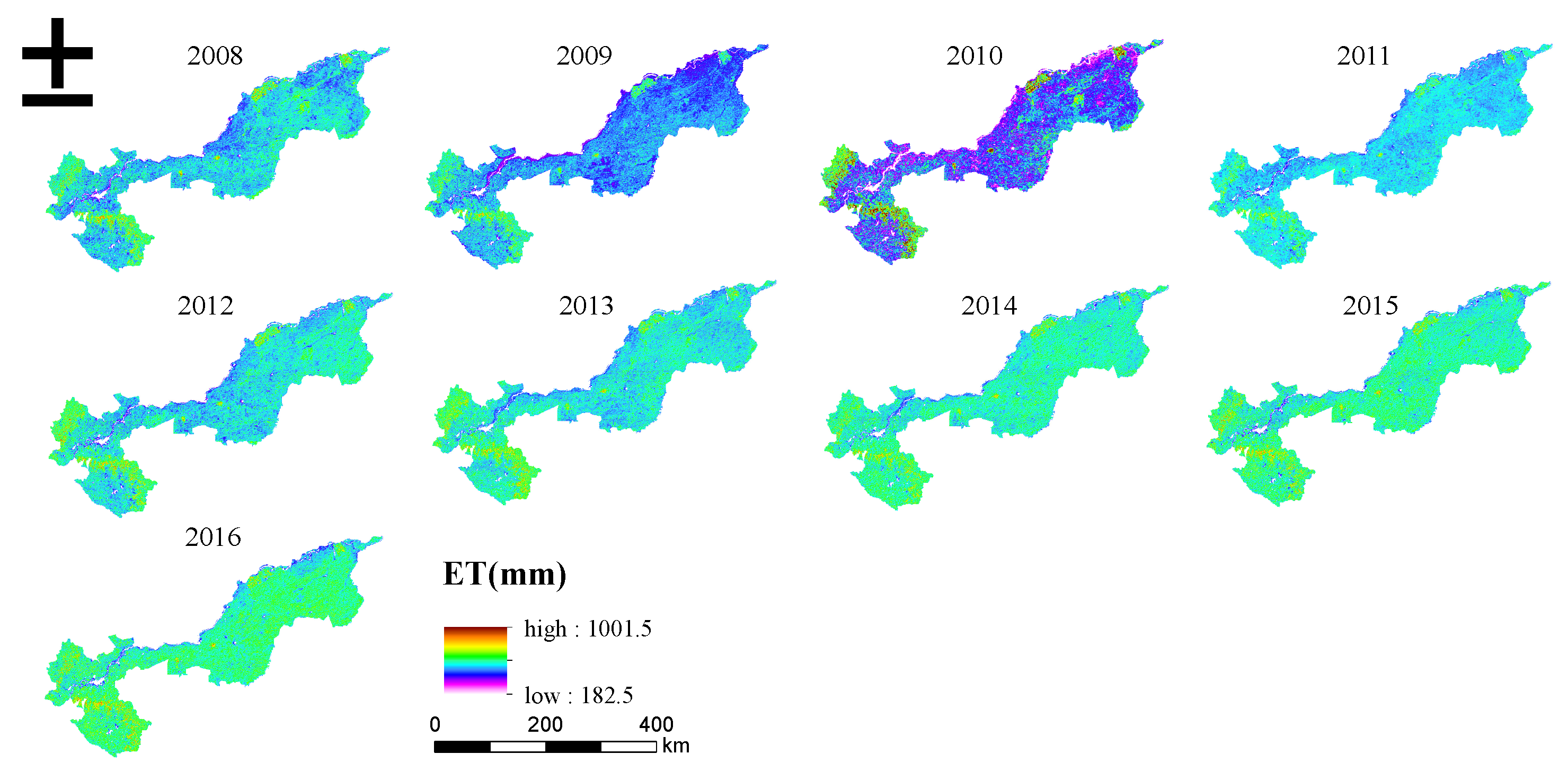
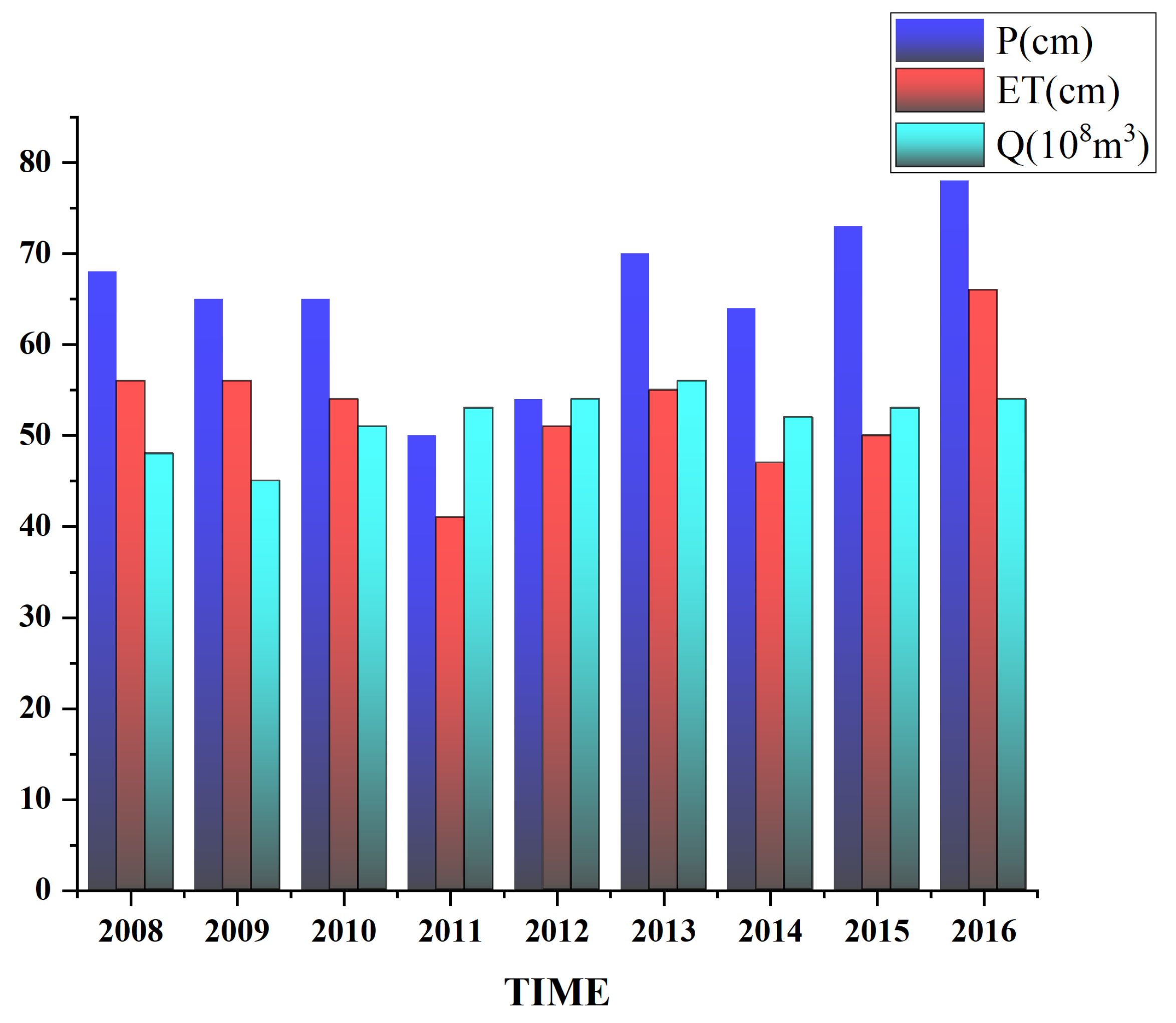
The groundwater recharge of the whole Jiamusi area from 2008 to 2016 was calculated by remote sensing, and the groundwater recoverable amount was calculated by using the average mining coefficient of different hydrogeological zones of Jiamusi City (ρ = 0.45), as shown in Table 7. The annual precipitation and evapotranspiration were obtained by TRMM and MOD16, and the detailed data are shown in Figure 5 and Figure 6: The average annual runoff depth was estimated by the GLDAS model, and the soil water storage in the research calculation area was = −1.5 mm. The relationship between groundwater recharge and precipitation evapotranspiration is shown in Figure 7.

4.2. Calculation of Groundwater Recharge in the Jiamusi Area by the SWAT Model

4.2.1. Sub-Watershed Division and HRU Unit

The sub-watershed division is a crucial component of the SWAT model’s simulation of surface runoff. The optimal water logging area threshold (22,579.14 Ha) was adopted in this link based on the imported DEM topographic map and the actual river system vector map. The entire outlet of the Tongjiang Hydrological Station in Tongjiang City and the Fuyuan Hydrological Station in Fuyuan City was selected automatically by the SWAT model. Subsequently, the No. 1 drainage basin was split into 31 sub-basins, and the No. 2 drainage basin was separated into 9 sub-basins via artificial adjustment. Every HRU constitutes the smallest underlying surface unit and is unique in terms of land use, soil composition, and slope division. The number of sub-basins, land use, soil type, topographic slope, and reclassification threshold value all affect the number of HRUs. In this work, the minimum area ratio of soil type and slope reclassification was 10%, and the land use of the two basins was established accordingly. Ultimately, 98 HRUs were created from the No. 1 basin and 31 HRUs from the No. 2 basin.

4.2.2. Parameter Calibration and Verification

Since the Jiamusi region is located in the cold temperate zone and the WAT model has many parameters, the parameters with the highest correlation sensitivity coefficient were chosen to modify the model’s parameters. The SWAT-CUP program was used to complete a sensitivity analysis of 22 parameters across two basins. Global sensitivity analysis was applied in this work. The model’s integrated SU-F2 sampling technique was used to perform 500 iterative calculations after the parameters and the initial range of selected parameters were established [27]. The model’s appropriateness was assessed using the Nash efficiency coefficient (NS) and determination coefficient (R2). Table 8 presents the ideal parameters.
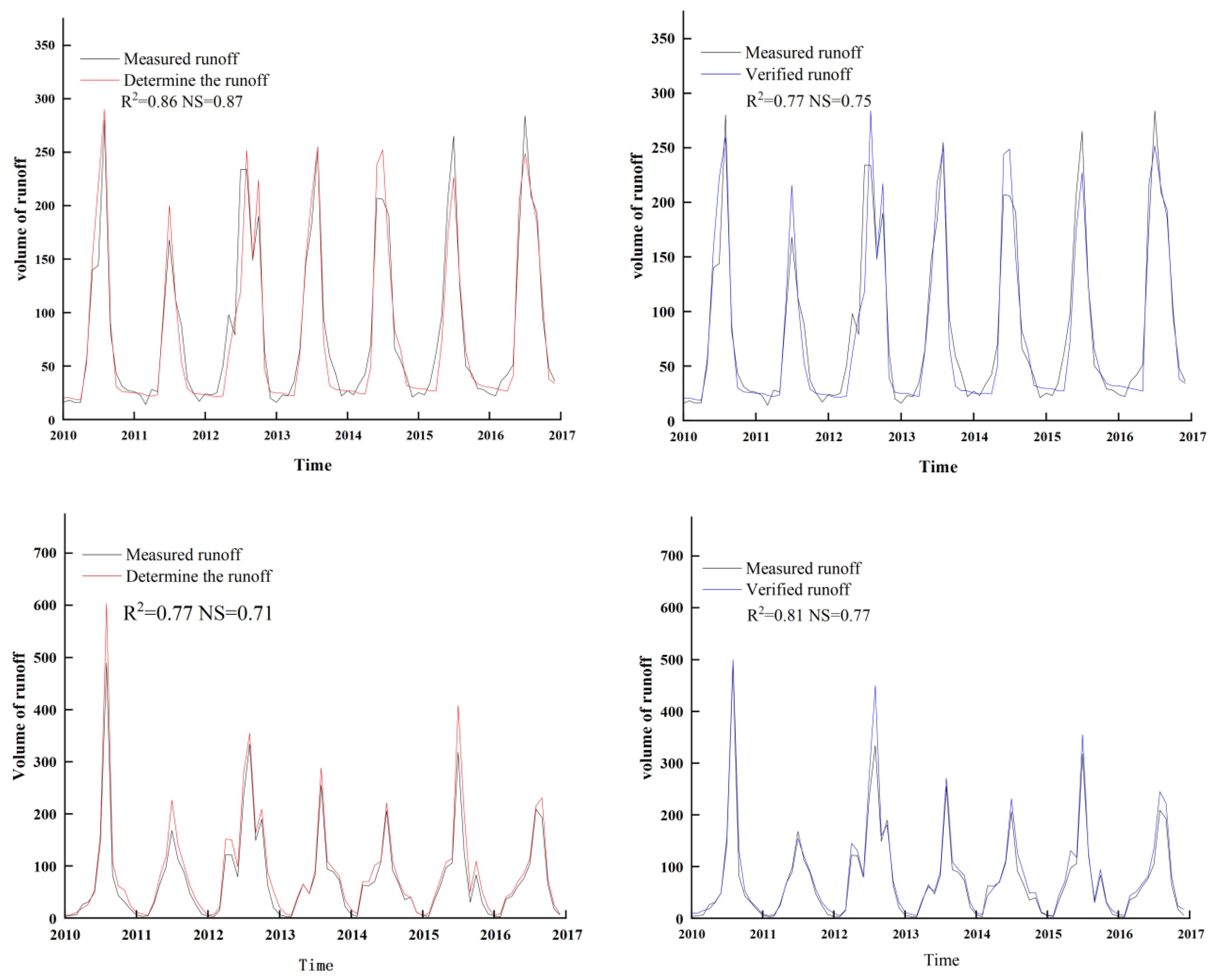
The spreadsheet was rewritten, and the validation was rerun after the corrected parameters were re-entered into the model. Figure 8 displays the findings of the verification and calculation of the runoff rate.
This time, the assessment parameters used were the Nash coefficient (NSE) and determination coefficient (R2), which are frequently employed in both local and international research. The better the effect, the closer the simulated value is to the observed value, the closer the secondary coefficient is to 1. Table 9 displays the reliability distribution under typical conditions.
According to the experimental findings, the runoff simulation at the Tongjiang Hydrological Station was optimal when R2 > 0.8 and NSE > 0.75. The runoff simulation’s R2 > 0.7 and NSE > 0.65 at the Fuyuan Hydrological Station were also good.

4.2.3. Calculation of Groundwater Resources Based on SWAT

The model’s simulation of the water reserves in the phreatic layer at the end of each year resulted in averages that were correlated with the sub-basins, as previously regionalized (refer to Figure 9). Overall, the groundwater reserves in the basin were distributed quite differently. Among these, Jiamusi City, the hub, showed the primary tendency of the No. 1 watershed, with the southeast direction rapidly falling. The primary cause is that agricultural planting occupies 75% of the area in the northeast and southeast, and a significant amount of irrigation water was required. Furthermore, the river’s main stem lies in the far southeast of the region; therefore, the available water supply is minimal. The primary trend of the No. 2 basin was declining from Fuyuan City in a southwesterly direction. This is primarily due to Fuyuan’s location in the basin’s entire exit, near Heilongjiang’s main river, which has a sizable lateral supply. The No. 1 basin’s southwest region is adjacent to Tongjiang City, and both have comparable groundwater storage capacities. Furthermore, the simulation findings’ net groundwater discharge trend was essentially in line with the real circumstances. As it moved from the center outward, drainage basin No. 1 gathers water in the southeast and northwest directions. The sub-drainage basins 1, 2, 3, and 5 of the Songhua River had very little water reserves in the phreatic layer, and the water resources were primarily surface water. Sub-basins No. 8 and No. 9 are situated in agricultural planting areas with significant groundwater withdrawals and are impacted by groundwater storage. Basin No. 2 diminishes from northeast to southwest.
Using groundwater balancing, groundwater storage characteristics in the Jiamusi area of the No. 1 and No. 2 watersheds were computed and summarized from 2010 to 2016 (two years of preheating) (see Table 10). It was evident that the Jiamusi area is over-exploited and that the average storage variable is −357 million m3/a. The biggest simulated runoff, with a storage variable of 1.416 billion m3/a, occurred in 2016. Positive equilibrium exists. Eighty-six percent of the groundwater in the drainage system comes from base flow recharged rivers. The lowest is the form loss of regression bag, which accounts for only 3.50%, and the second is approximately 13.85%, mostly because of the refilling of deep aquifers. Plant roots’ absorption of water from shallow water levels is the primary cause of water loss. The Jiamusi region has a wide yearly temperature variation and a temperate continental climate. Evapotranspiration and rainfall differ too much from one another. The Songhua River basin’s potential emission increase is expected to rise in the twenty-first century. The area is mostly renewed by atmospheric precipitation, although there are a number of surface-level variables that contribute to the inadequate replenishment. The principal causes are the extended duration of the winter season, the frozen river, and the substantial groundwater supply to the river.
Because of the intricate geology of the Jiamusi area and the disparate hydrogeological conditions of each molecular basin, the evaluation of water resources was based on the division of molecular basins and the characteristic hydrological year. Monthly measured runoff data from 2009 to 2018 were chosen from the Tongjiang Hydrology Station, which is the entire downstream of the No. 1 basin. The general dry year 2011 (p = 75%) was synthesized using the empirical frequency analysis approach, with an annual discharge of 662 million m3. The yearly runoff was 981 million m3 in 2014 (p = 50%) and 1.216 billion m3 in 2016 (p = 25%). The recoverable amount of groundwater was computed in average years. This paper computed the natural recharge of the groundwater system in the watershed using the groundwater runoff modulus approach. Prior to calculating the natural recharge of each sub-basin, the output of each sub-basin in a typical year that the model simulated was determined. The average runoff of each sub-basin was then translated into the groundwater runoff modulus of each sub-basin. Moreover, the groundwater exploitable amount in typical years of each sub-basin was estimated using the exploitable coefficient approach in order to determine the groundwater exploitable amount in the basin at the scale of the research region. The average mining coefficient (ρ = 0.45) of the several hydrogeological zones in Jiamusi City was calculated in order to increase the estimation’s accuracy. It can be seen from the calculation that the groundwater recharge in the No. 1 basin was about 384,925,200 cubic meters in the dry year, about 46,580,908,600 cubic meters in the normal year, and 4,801,663,100 cubic meters in the wet year; therefore, the groundwater recharge in the wet year was 1.25 times that in the dry year. The trend of groundwater recharge in the No. 2 basin was similar to that in the No. 1 basin. The groundwater recharge in the dry year was 841,353,600 cubic meters, the groundwater recharge in the normal year was about 1,883,781,800 cubic meters, and the groundwater recharge in the wet year was about 2,350,304 million cubic meters; therefore, the groundwater recharge in the wet year was about 2.54 times that in the dry year. Detailed results are shown in Table 11 and Table 12 and Figure 10.

5. Discussion

5.1. Applicability of SWAT Model and Remote Sensing Meteorology to Groundwater Recharge Calculation

At present, the groundwater dynamic balance, rainfall infiltration coefficient, and water balance methods are the three main methods for calculating groundwater recharge [28]. These technologies are well-developed and have been widely used in both practical work and scientific research. For the water balance and rainfall infiltration coefficient methods, the scope of application is wider, and the review process is more straightforward [29]. However, the traditional calculation formula relies on the field observation data. For example, the dynamic groundwater level method requires more field groundwater level observation well data, which requires huge manpower and time to obtain. However, the SWAT model is very effective in studying how people live, how the climate changes, and what surface runoff and groundwater look like [30]. In addition, the data required by this model are easy to obtain, and impact can also be eliminated by adjusting parameters for other environmental impact factors. In addition, the model further subdivides the geographical, meteorological, and hydrological data of each unit on the basis of the division of hydrological units. Local uniformity can be achieved through physical processes such as recharge, evaporation, throttling, and infiltration of water resources in the area. This can effectively solve the problem of insufficient accuracy in water resource calculations caused by hydrogeological differences [31].
Groundwater level observation wells and other nearly ideal water conservation facilities are the foundation of the dynamic technique of groundwater level [32]. It is expensive and labor-intensive. The remote sensing-based water balance approach offers several advantages over the dynamic groundwater level method, including the ability to integrate RS GIS and a worldwide road surface data assimilation system. In addition, these technical approaches represent current areas of interest for study and development [33]. Data capture is, therefore, quicker and more convenient. Remote sensing compensated for the absence of conventional monitoring stations in the mountainous regions, difficult topography, and significant data inaccuracies in the Jiamusi area. Furthermore, remote sensing has a low temporal precision and a large coverage area. The rainfall infiltration coefficient approach’s disregard for the balance method based on remote sensing significantly reduces the impact of these effects on geological water storage and runoff [34]. It significantly increased the accuracy of groundwater recharge in Jiamusi, a location with complicated geology and an intricate water infrastructure.

5.2. Current Deficiencies and Prospects for Future Improvement

The SWAT model has been developed over a considerable amount of time—more than 20 years from 1990 to the present. It is also semi-distributed, making it simpler to learn and comprehend than completely distributed models. Simultaneously, the rate of calculation is accelerated, and the accuracy is improved, better reflecting the physical mechanism of the water cycle than the conceptual model [35]. However, the model’s description of the water cycle mechanism—such as irrigation and submersible evaporation—is not as good as it may be when compared to other hydrological models. Furthermore, there is a low degree of modularity, a large number of input files that are difficult to handle, and a source program that is difficult to learn and alter (there are over 300 FORTRAN source programs). This paper’s research focus was northeast China, where four distinct seasons cause notable climate variations. The groundwater recharge and discharge relationship simulation findings in the winter have a wide range and poor precision. To lessen the impact of temperature on the coupling model, the SWAT and MODFLOW models should be coupled [36,37], the LU-SWAT-MODFLOW model should be created, and a range of data should be merged to calibrate and validate the coupling model. Additionally, dynamic land use input should be introduced to the model since dynamic updating of land use data is necessary to re-determine the threshold value during the simulation process, which is highly unfavorable in places with changeable soil.
In general, the hydrologic data required for it to work cannot be directly gathered; instead, inverse observation is required. Remote sensing observation is a type of indirect observation.
It is impossible to prevent errors in rededuction precision [38,39]. Remote sensing rainfall, in particular, is only more accurate on a monthly scale, with significant error on a day-by-day and hour-by-hour basis. Second, there is a significant inaccuracy in the predicted groundwater recharge because remote sensing is unable to monitor the evapotranspiration of inland water bodies. Future scientific research projects should include the relative error coefficient in the final calculation formula.

6. Conclusions

  • The HWSD World Soil Database and the CMADS meteorological data set, which serve as the model’s driving databases, simulated the study region well. With R2 and NS values of 0.81 and 0.77, respectively, Fuyuan Hydrology Station had the best simulation effect. Tongjiang Hydrology Station followed with R2 and NS values of 0.77 and 0.75, respectively, both of which meet the simulation requirements.
  • Examine the entire scene. In the Jiamusi area, groundwater phreatic-bed reserves are distributed very differently. The primary pattern is the progressive decrease in volume in Jiamusi city to the northeast and southeast. It falls to the southwest of Fuyuan City’s center. The trend of the simulated groundwater net discharge is essentially in line with reality. The Songhua River trunk area in Tongjiang City contains the Jiamusi groundwater storage area to the southeast and northwest. Surface water makes up the majority of the water resources here, with relatively little water reserves in the diving layer. Jiamusi’s northeast primarily diminishes to the southwest from Fuyuan City’s core.
  • The average groundwater recharge in the Jiamusi area between 2008 and 2016 was estimated by the remote sensing water balance method to be 53.2 × 10⁸ m3, while the average exploitable amount was found to be 23.94 × 10⁸ m3. The recoverable amount was 27.4 × 10⁸ m3, and the average groundwater recharge was 61.03 × 10⁸ m3, according to the SWAT model. Between 2010 and 2016, the No. 1 basin’s average groundwater runoff modulus was 0.89 L/(s·km2), total recharge was 31.522 billion m3, and total recoverable amount was 14.184 billion m3. In the No. 2 basin, the total recharge was 11.256 billion m3, the total recoverable amount was 5.065 billion m3, and the average groundwater runoff modulus was 1.113 L/(s·km2).
  • Given the restoration of Jiamusi’s groundwater level, it is recommended that flood waters be released in the upper reservoir of the Shidang River during dry years in order to maintain Songhua River’s water level stability and lessen groundwater reversal recharge while providing irrigation water for the Fujin Irrigation District. In rural regions, it is suggested that supervision over groundwater consumption for agriculture and irrigation is tightened, awareness is increased, and the bar for groundwater use is raised.

Author Contributions

Conceptualization, X.Y.; Methodology, X.Y.; Software, X.Y.; Validation, X.Y.; Formal analysis, X.Y.; Data curation, C.L.; Writing—original draft, X.Y.; Writing—review & editing, C.D. and G.L. All authors have read and agreed to the published version of the manuscript.

Funding

This research was funded by: (1) [Research and analysis of Sino-Russian glacial flow measurement technology in Heilongjiang (Amur River) and suggestions on survey schemes]. (2) [Yunnan Key Laboratory of International Rivers and Transboundary Eco-Security] grant number [2022KF03] and the APC was funded by [2022KF03].

Data Availability Statement

The original contributions presented in the study are included in the article, further inquiries can be directed to the corresponding author.

Conflicts of Interest

The author hereby declares no conflict of interest.

References

  1. Ning, L.; Pan, T.; Zhang, Q.; Zhang, M.; Li, Z.; Hou, Y. Differentiated Impacts of Land-Use Changes on Landscape and Ecosystem Services under Different Land Management System Regions in Sanjiang Plain of China from 1990 to 2020. Land 2024, 13, 437. [Google Scholar] [CrossRef]
  2. Kang, L.; Zhang, H.Q. Sensitivity Analysis of the Evaluation of Agricultural Drought Resistance Capacity in China’s Five Major Grain-Producing Regions. J. China Agric. Univ. 2015, 20, 214–224. [Google Scholar]
  3. Zhang, H.; Zhang, Y.D.; Huang, Y.; Wang, B. Study on Water Consumption Patterns and Growth Characteristics of Rice under Different Irrigation Modes. Water Sav. Irrig. 2023, 4, 25–31. [Google Scholar]
  4. Wu, W.J.; Xia, T.; Hu, Q. Pattern of Conversion between Paddy Fields and Dry Lands and Its Water Resource Effects in Heilongjiang from 1980 to 2015. China Agric. Resour. Reg. Plan. 2019, 40, 142–151. [Google Scholar]
  5. Zhang, M.N.; Cheng, X.X.; Li, Z.H.; Liu, W.P.; Cui, H.Q.; Wei, S.B.; Liu, W.P.; Liu, J.T.; Li, Y.L.; Chen, Z. Monitoring, Assessment, and Prediction of Ground Surface Deformation in the Groundwater Level Decline Area of Jiansanjiang in Sanjiang Plain. Geol. Bull. 2023, 42, 1211–1217. [Google Scholar]
  6. DeMille, M. Assessment and estimation of groundwater recharge for a catchment located in highland tropical climate in central Ethiopia using catchment soil–water balance (SWB) and chloride mass balance (CMB) techniques. Environ. Earth Sci. 2015, 74, 1137–1150. [Google Scholar] [CrossRef]
  7. Hornero, J.; Manzano, M.; Ortega, L.; Custodio, E. Integrating soil water and tracer balances, numerical modelling and GIS tools to estimate regional groundwater recharge: Application to the Alcadozo Aquifer System (SE Spain). Sci. Total Environ. 2016, 568, 415–432. [Google Scholar] [CrossRef]
  8. Yin, L. Study on Groundwater Recharge Based on Multiple Methods; China University of Geosciences: Beijing, China, 2011. [Google Scholar]
  9. Cheng, K. Regional Optimal Allocation of Land and Water Resources and Risk Analysis of Food Security Based on Complex Adaptive System Theory. Ph.D. Thesis, Northeast Agricultural University, Harbin, China, 2015. [Google Scholar]
  10. Zhao, Q.; Tang, J.; Yang, H.; Zhang, X.L.; Luo, L.J. The chronology and geochemical characteristics of Late Triassic Adakite in central Jimusi Block and its geological significance. J. Earth Sci. Environ. 2019, 45, 240–255. [Google Scholar]
  11. Liu, R. Study on the Comparative Advantages of Developing Modern Agriculture in Jiamusi City and Sanjiang Plain. Stat. Consult. 2015, 3, 24–26. [Google Scholar]
  12. Zhao, X.G. Prediction of Mine Water Inflow Based on Atmospheric Rainfall Infiltration Coefficient Method and Kosyakov Formula. Inn. Mong. Coal Econ. 2014, 137+141. [Google Scholar] [CrossRef]
  13. Yun, Z.D.; Hu, Q.F.; Wang, Y.T.; Wu, H.Y.; Wang, L.Z.; Shang, S.W. Accuracy Assessment of Remote Sensing and Reanalysis Evapotranspiration Data: A Comparative Study Based on GRACE and Basin Monthly Water Balance Model. J. Hydraul. Eng. 2023, 54, 117–127. [Google Scholar] [CrossRef]
  14. Liang, Z.M.; Zhao, J.F.; Duan, Y.N.; Huang, J.; Li, B.; Wang, J.; Hu, Y. Differential form New Anjiang model. Adv. Water Sci. 2024, 35, 374–386. [Google Scholar]
  15. Kong, C.; Zhang, H.Y.; Dai, J.F.; Lv, Y.J.; Li, Z.T.; Wan, Z.P. Runoff simulation of Musong River Basin in Huixian rock-soluble wetland based on tank model. Yellow River 2019, 46, 17–21+63. [Google Scholar]
  16. Zhu, C.H. Optimal Allocation of Water Resources in Jiamusi City Based on Multidimensional Critical Regulation Theory; Northeast Agricultural University: Harbin, China, 2015. [Google Scholar]
  17. Ridwansyah, I.; Yulianti, M.; Apip, O.S.I.; Shimizu, Y.; Wibowo, H.; Fakhrudin, M. The impact of land use and climate change on surface runoff and groundwater in Cimanuk watershed, Indonesia. Limnology 2020, 21, 487–498. [Google Scholar] [CrossRef]
  18. Zhu, Y.F. Study on Water Resource Vulnerability in Songhua River Basin under Changing Environment; Jilin University: Changchun, China, 2024. [Google Scholar]
  19. Chen, K.; Wang, L.Q.; Liu, Y.; Liu, J.X. Applicability evaluation of CMADS dataset in Hulan River Basin. J. Irrig. Drain. 2019, 43, 60–68. [Google Scholar]
  20. Aqnouy, M.; Ommane, Y.; Ouallali, A.; Gourfi, A.; Ayele, G.T.; El Yousfi, Y.; Bouizrou, I.; Stitou El Messari, J.E.; Zettam, A.; Melesse, A.M.; et al. Evaluation of TRMM 3B43 V7 precipitation data in varied Moroccan climatic and topographic zones. Mediterr. Geosci. Rev. 2024, 6, 159–175. [Google Scholar] [CrossRef]
  21. Abid, N.; Jaafar, B.A.; Bargaoui, Z.; Mannaerts, C.M. Assessment of long term MOD16 and LSA SAF actual evapotranspiration using Budyko curve. Remote Sens. Appl. Soc. Environ. 2024, 34, 101166. [Google Scholar]
  22. Gautam, K.P.; Chandra, S.; Henry, K.P. Monitoring of the Groundwater Level using GRACE with GLDAS Satellite Data in Ganga Plain, India to Understand the Challenges of Groundwater Depletion, Problems, and Strategies for Mitigation. Environ. Chall. 2024, 15, 100874. [Google Scholar] [CrossRef]
  23. Chen, Y.H.; Li, X.B.; Shi, P.J. The Remote Sensing Model for Regional Evapotranspiration Estimation over Heterogeneous Landscape. Acta Meteorol. Sin. 2002, 60, 508–512. (In Chinese) [Google Scholar]
  24. Zhang, W.M.; Dong, Z.C.; Qian, W.; Zhu, C.T. Advances in Applications of Remote Sensing Data to Hydrology and Water Resources. Water Sav. Irrig. 2007, 8, 24–32. (In Chinese) [Google Scholar]
  25. Zhao, X.L.; Yan, X.D. Study on the Change Trend of Soil Water Storage in Heilongjiang Province in the Past 20 Years. Geogr. Sci. 2006, 5, 5569–5573. [Google Scholar]
  26. Wang, Z.G.; Liu, C.M.; Huang, Y.B. Research on the principle, structure and application of SWAT model. Prog. Geogr. 2003, 1, 79–86. [Google Scholar]
  27. Saurette, D.D.; Biswas, A.; Gillespie, A.W. Determining minimum sample size for the conditioned Latin hypercube sampling algorithm. Pedosphere 2024, 34, 530–539. [Google Scholar] [CrossRef]
  28. Abdo, H.G.; Vishwakarma, D.K.; Alsafadi, K.; Bindajam, A.A.; Mallick, J.; Mallick, S.K.; Kumar, K.C.A.; Albanai, J.A.; Kuriqi, A.; Hysa, A. GIS-based multi-criteria decision making for delineation of potential groundwater recharge zones for sustainable resource management in the Eastern Mediterranean: A case study. Appl. Water Sci. 2024, 14, 160. [Google Scholar] [CrossRef]
  29. Zhang, J.Z.; Zhang, Z.Y.; Wang, Q.M. Study on rainfall infiltration recharge law of typical small watershed in Hebei Plain. J. China Inst. Water Resour. Hydropower Res. 2023, 21, 37–46. (In Chinese) [Google Scholar]
  30. Liu, K.; Li, M.J.; Mou, H.L.; Lv, Z.Y.; Liu, P.; Yin, Z.K.; Liu, Z.W.; Liang, L.L. Analysis of influential factors in large-scale runoff simulation by SWAT model: A case study of the upper Parana River Basin. J. Water Resour. Archit. Eng. 2019, 21, 191–198. [Google Scholar]
  31. Mebarki, H.; Maref, N.; Dris, A.E.M. Modelling the monthly hydrological balance using Soil and Water Assessment Tool (SWAT) model: A case study of the Wadi Mina upstream watershed. J. Groundw. Sci. Eng. 2019, 12, 161–177. [Google Scholar] [CrossRef]
  32. Zhu, Q.; Zhao, H.Y.; Wang, J.Y.; Liu, T.W. The underground water level dynamic change characteristics and influencing factors analysis. Water Beijing 2024, 3, 1–6. [Google Scholar] [CrossRef]
  33. Chen, J.M. An important shortcoming and improvement of evapotranspiration model in current remote sensing. Chin. Sci. Bull. 1988, 6, 454–457. [Google Scholar]
  34. Hinzer, I.; Altherr, M.; Christiansen, R.; Schreuer, J.; Wohnlich, S. Characterisation of an Artesian Groundwater System in the Valle de Iglesia in the Central Andes of Argentina. Int. J. Earth Sci. 2021, 110, 2559–2571. [Google Scholar] [CrossRef]
  35. Yao, R. Study on the Dynamics and Prediction of Groundwater Level in the Urban Area of Jiamusi City; Heilongjiang University: Harbin, China, 2024. [Google Scholar]
  36. Uwamahoro, S.; Liu, T.; Nzabarinda, V.; Muhigire, J.; Umugwaneza, A.; Maniraho, A.P.; Ingabire, D. Assessing hydrological interactions, soil erosion intensities, and vegetation dynamics in Nyabarongo River tributaries: A SWAT and RUSLE modeling approach. Model. Earth Syst. Environ. 2024, 10, 4317–4335. [Google Scholar] [CrossRef]
  37. Ayalew, B.Y.; Seoro, L.; Jae, K.L. Calibration and uncertainty analysis of integrated SWAT-MODFLOW model based on iterative ensemble smoother method for watershed scale river-aquifer interactions assessment. Earth Sci. Inform. 2023, 16, 3545–3561. [Google Scholar]
  38. Ji, X.Y.; Wei, Y.C.; Wang, W.Y.; Fang, H. Error Analysis of Surface Cover Change Detection in Urban Areas Using High-Resolution Remote Sensing Images. Remote Sens. Technol. Appl. 2018, 33, 932–941. [Google Scholar]
  39. Yu, Y. Study on the Impact of Water Resources Utilization on Aquatic Ecology in Jinxi Irrigation Area of Fujin City, Heilongjiang Province. Sci. Technol. Innov. 2020, 10, 118–119. [Google Scholar]
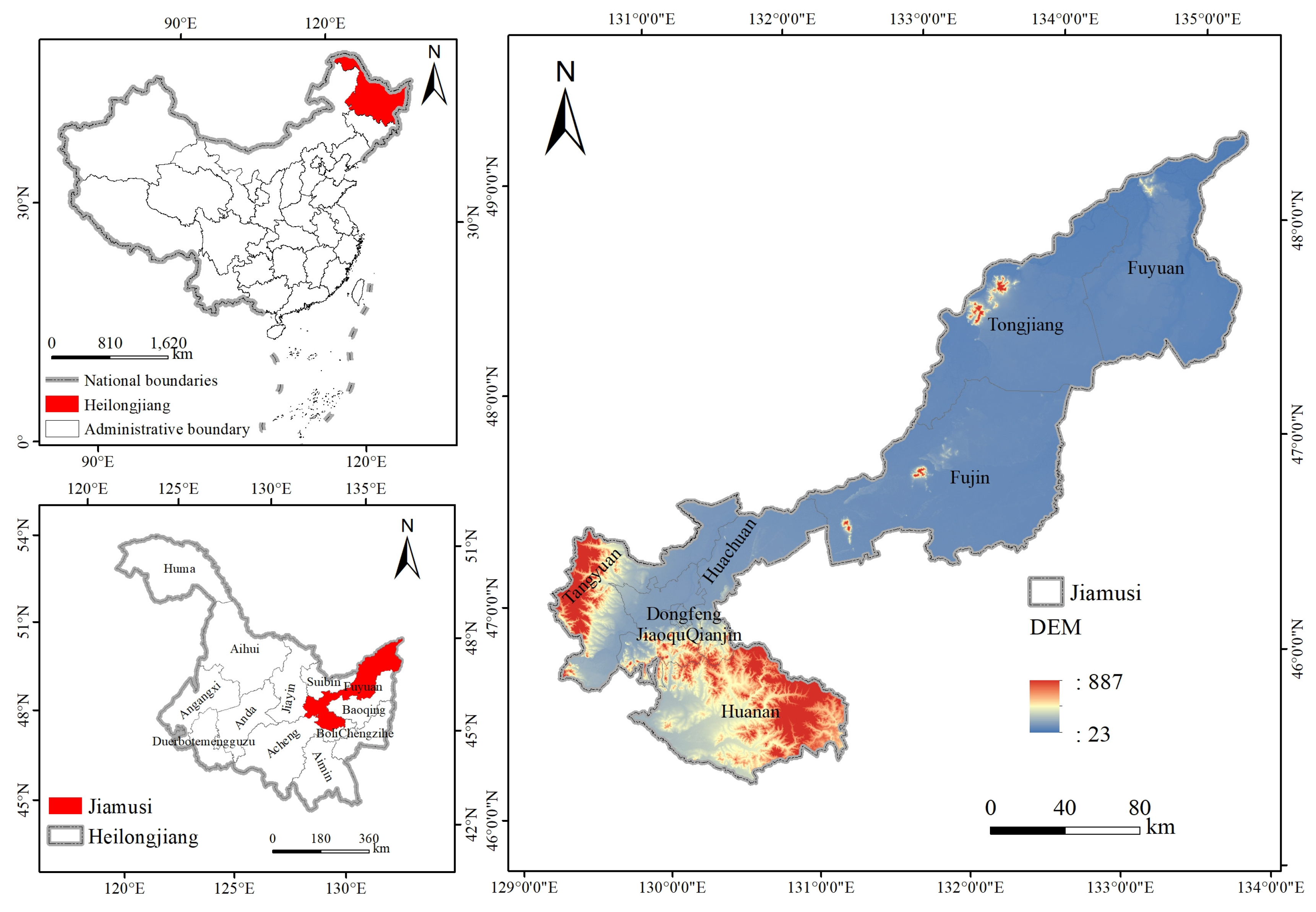
Figure 1. Jiamusi area geographic survey map.
Applsci 14 07220 g001
Figure 2. The basin’s geographical location.
Applsci 14 07220 g002
Figure 3. Schematic diagram of sub-watershed division, soil type reclassification, and land use reclassification in the calculation area (AC) represents No. 1 watershed, (ac) represents No. 2 watershed. (The numbers in (A) and (a) are the serial numbers of sub-basins divided by SWAT model).
Applsci 14 07220 g003
Figure 4. Technology roadmap. (I indicates the optimal parameter range for the first run of the model lock, II indicates that the parameter range is shortened for rerun).
Applsci 14 07220 g004
Figure 5. Precipitation distribution map of Jiamusi from 2008 to 2016 (P is precipitation Unit: mm).
Applsci 14 07220 g005
Figure 6. Evapotranspiration layout of Jiamusi from 2008 to 2016 (ET represents evapotranspiration Unit: mm).
Applsci 14 07220 g006
Figure 7. Relationship among groundwater recharge, precipitation and evapotranspiration. (ET represents annual average evapotranspiration, Q represents groundwater recharge, and P represents precipitation).
Applsci 14 07220 g007
Figure 8. Determination and verification of the runoff model (the above two pictures are the simulation results of Tongjiang Hydrology Station, and the next two pictures are the simulation results of Fuyuan Hydrology Station. The ordinate indicates the amount of runoff. Unit: m3, the horizontal coordinate is the year).
Applsci 14 07220 g008
Figure 9. Spatial distribution map of water volume in phreatic beds in sub-basins ((a) is basin No. 1, (b) is basin No. 2, Unit: 108 × m3).
Applsci 14 07220 g009
Figure 10. Groundwater recharge and recoverable amount in the basin (SUP is groundwater recharge amount, EXP is groundwater recoverable amount, Unit: 108 m3).
Applsci 14 07220 g010
Table 1. Main soil types as a percentage.
Soil TypeFLCPHhGLMATcLVhCMe
Watershed No. 12.1225.237.192.8815.170.35
Watershed No. 23.4428.988.71-16.560.44
Table 2. Soil coefficient and level calculated by SPAW (No. 1 watershed).
CoefficientSOL_BD1SOL_AWC1SOL_K1SOL_CBN1SOL_BD2SOL_AWC2SOL_K2SOL_CBN2Hierarchy
Soil Type
FLc1.520.149.320.631.470.1412.600.47L-L
PHh1.350.1414.211.901.590.138.210.67L-L
GLm1.490.1413.551.621.590.145.200.65L-CL
ATc0.970.1943.521.151.430.148.930.80SIL-L
LVh1.530.1310.330.701.620.134.140.35L-CL
CMe1.470.1410.211.111.510.125.730.31L-L
WATER1.70025800000-
Table 3. Soil coefficient and level calculated by SPAW (Basin No. 2).
CoefficientSOL_BD1SOL_AWC1SOL_K1SOL_CBN1SOL_BD2SOL_AWC2SOL_K2SOL_CBN2Hierarchy
Soil Type
FLc1.650.179.350.671.450.1412.570.41L-L
PHh1.370.1213.211.791.630.149.010.55L-L
GLm1.640.1413.511.281.620.145.550.54L-CL
LVh1.590.1310.490.771.590.134.270.57L-CL
CMe1.390.149.171.171.480.147.340.28L-L
WATER1.98028800000-
Table 4. Related descriptions of soil coefficients involved in the calculation of SPAW.
CoefficientDescriptionCoefficientDescription
SOL_BDweight of dried soil, comprising soil particles and intergranular pores, per unit volume. It stands for the moist bulk density of soil (SOILdensity).CLAYClay content, %wt, refers to soil particles <0.002 mm in diameter.
SOL_AWCIndicates the effective water content of the soil layer in mm/mm.SILTSilt refers to the loam content of the soil (%wt); that is, the percentage by weight of soil particles between 0.002 and 0.05 mm in diameter.
SOL_CBNOrganic carbon content (%wt) of the soil layer.SANDSand content, %wt, refers to particles with diameters between 0.05 and 2.0 mm.
SOL_KSaturated water conductivity/saturated hydraulic conductivity, mm/h.ROCKGravel content, %wt, refers to particles with a diameter greater than 2 mm;
SOL_ZMSRepresents the maximum root depth of the soil profile, mm.USLE_KErodibility factor
Table 5. SWAT code of land use.
Reclassification CodingNameSWAT Coding
1PlowlandAGRL
2Forest landFRST
3MeadowRNGB
4WaterWATR
5Urban and rural, industrial and mining, residential landURML
6Unused landWETL
Table 6. Basic geographic data required.
Data TypeData Source
Digital Elevation Model (DEM)NASA Earth Science data website (https://nasadaacs.eos.nasa.gov/) accessed on 15 June 2024
Soil type and attribute listHWSD data downloaded from the National Tibetan Plateau Scientific Data Center (World Soil Database) (https://data.tpdc.ac.cn/home) accessed on 15 June 2024
Land type use dataInstitute of Aerospace Information Innovation, Chinese Academy of Sciences
Meteorological dataCMADS (V1.1) downloaded from the National Tibetan Plateau Scientific Data Center (https://data.tpdc.ac.cn/home) accessed on 15 June 2024
Runoff dataTongjiang City Hydrology Station
Precipitation dataTRMM data
EvapotranspirationMOD16 software synthesis
Surface runoff depthGLDAS model estimation
Table 7. Groundwater recharge and extraction in the Jiamusi Area from 2008 to 2016, calculated by the remote sensing water balance method (108 m3).
A Given Year200820092010201120122013201420152016Mean Value
Supplemental amount56.354.555.840.551.856.745.550.567.7153.2
Recoverable amount25.324.525.118.223.325.520.422.730.423.94
Table 8. Sensitivity analysis table of parameters.
EncodingParameter NameParameter MeaningOptimal Parameter (Basin No. 1)Optimal Parameter (Basin No. 2)
1r__CN2.mgtSCS runoff curve value0.750.81
2v__GW_DELAY.gwGroundwater delay time784.90721.10
3v__GWQMN.gwLevel threshold of shallow aquifers when groundwater enters the main channel (mm)2.011.88
4v__REVAPMN.gwShallow groundwater evaporation depth threshold (mm)900.40855.50
5v__SOL_AWC().solSurface water availability (mm)−0.441.02
6v__CH_K2.rteEffective permeability coefficient (mm/h)695.11721.41
7v__RCHRG_DP.gwPermeability coefficient of deep aquifer0.550.53
8r__SOL_K().solSoil-saturated water conductivity (mm/h)1.601.45
9r__SOL_ALB().solMoist soil albedo0.310.35
10v__ALPHA_BNK.rteBase flow regression constant0.240.24
11v__SLSUBBSN.hruAverage slope length (m)1.952.11
12r__HRU_SLP.hruAverage slope (m/m)2.332.16
13v__CANMX.hruMaximum canopy water storage (mm)427.5455.4
14v__SFTMP.bsnAverage air temperature on snowfall days (°C)10.09.12
15v__SMTMP.bsnAverage temperature on snowfall days (°C)13.812.44
16v__SMFMX.bsnSnowmelt factor35.045.50
17v__TIMP.bsnTemperature lag coefficient of snow cover2.842.58
18v__SNOCOVMX.bsnSnow depth threshold/cm1002.29800.50
19v__TLAPS.subTemperature lapse rate (°C/km)4.443.58
20v__ESCO.hruSoil evaporation compensation coefficient1.532.00
21v__EPCO.hruPlant absorption compensation coefficient0.710.85
22v__ALPHA_BF.gwBase flow alpha factor (1/day)1.251.47
Table 9. R2 and NSE confidence comparison table.
Model ReliabilityR2NSE
equivalent to gold0.80 < R2 ≤ 1.000.75 < NSE ≤ 1.00
excellent0.70 < R2 ≤ 0.800.65 < NSE ≤ 0.75
typical0.50 < R2 ≤ 0.700.50 < NSE ≤ 0.65
Not happyR2 ≤ 0.50NSE ≤ 0.50
Table 10. Groundwater storage variables in Jiamusi area. Unit: 108 m3.
A Given YearSupply TermExcretion TermSubtotal∆Sgw
PERCREVAPGWQDARCHG
201035.703.626.1512.516.56−6.56
201126.403.4131.217.6125.82−25.82
201242.502.0730.411.528.58.5
201333.540.4235.642.004.34−4.34
201435.420.2339.091.835.73−5.73
201529.77033.081.755.13−5.13
201651.590.1135.761.5614.1614.16
Mean value36.411.4033.045.543.57−3.57
Excretion item percentage/%-3.5082.6413.85--
Table 11. Subsurface runoff modulus, recharge, and recoverable amount in the sub-basins of No. 1 basin.
SubcatchmentDry Year (2011)Normal Water Year (2014)Wet Year (2016)
Runoff Modulus (l·s−1·km2)Supply (104 m3·a−1)Recoverable Amount
(104 m3·a−1)
Runoff Modulus (l·s−1·km2)Supply (104 m3·a−1)Recoverable Amount
(104 m3·a−1)
Runoff Modulus (l·s−1·km2)Supply (104 m3·a−1)Recoverable Amount
(104 m3·a−1)
10.32738.89332.500.352878.461295.310.322864.861289.19
20.325001.232250.550.445124.132305.860.394639.692087.86
30.297324.103295.850.396956.443130.400.417357.463310.86
40.795135.032310.760.644921.602214.720.655677.382554.82
50.534408.691983.910.575307.092388.190.606025.342711.40
60.18582.45262.100.31819.46368.760.25772.87347.79
71.1820,504.179226.881.3926,464.7811,909.151.2025,084.8011,288.16
80.956765.133044.311.088005.843602.631.139033.714065.17
91.168058.633626.381.269011.324055.091.218980.724041.32
101.0719,627.648832.441.1013,622.536130.141.0914,704.896617.20
110.101227.11552.200.10787.08354.190.12815.17366.83
120.263222.561450.150.171160.80522.360.171225.64551.54
131.0318,993.388547.021.0415,421.416939.631.0417,147.587716.41
140.355539.7217.870.426738.713032.420.427169.693226.36
150.394000.181800.080.426738.713032.420.427169.693226.36
160.081248.72561.920.202211.69995.260.181604.62722.08
171.2085,096.9038,293.611.29101,863.3745,838.521.28110,336.7049,651.52
180.9215,048.286771.731.0318,687.938409.570.9518,368.968266.03
190.1392.7941.760.15107.7548.490.16119.9453.97
200.12446.01200.700.313056.161375.270.323169.521426.28
210.351052.07473.430.411274.18573.380.421402.29631.03
220.9257,196.0625,738.231.1265,089.9129,290.461.1568,030.4130,613.68
230.242688.071209.630.273262.561468.150.993592.441616.60
240.391280.56576.250.481512.85680.780.471535.84691.13
250.8725,076.7511,284.540.9730,075.7813,534.100.9633,043.8914,869.75
260.235775.522598.980.408236.073706.230.438826.073971.73
271.1423,876.8110,744.561.2125,737.7911,582.011.1323,683.2310,657.45
280.4813,511.606080.220.7919,511.938780.370.7219,146.638615.98
290.4311,758.905291.510.7515,138.606812.370.7013,377.216019.74
300.336701.983015.890.469354.134209.360.438663.023898.36
311.0728,442.5912,799.171.2836,532.7416,439.731.1831,865.5814,339.51
total-384,922.52173,215.13-465,890.86209,650.89-480,166.31216,074.84
Table 12. Subsurface runoff modulus, recharge, and exploitable amount in the sub-basins of No. 2 basin.
SubcatchmentDry Year (2011)Normal Water Year (2014)Wet Year (2016)
Runoff Modulus (l·s−1·km2)Supply (104 m3·a−1)Recoverable Amount
(104 m3·a−1)
Runoff Modulus (l·s−1·km2)Supply (104 m3·a−1)Recoverable Amount
(104 m3·a−1)
Runoff Modulus (l·s−1·km2)Supply (104 m3·a−1)Recoverable Amount
(104 m3·a−1)
10.441033.81465.210.541168.31525.730.581457.64655.93
20.435441.232448.550.536201.792790.800.627737.663481.94
31.137825.903521.651.3990,358.0540,661.121.61112,735.2250,730.84
41.0915,532.006989.41.3520,557.539250.881.4225,648.6011,541.87
50.888938.804022.461.0911,851.045332.961.0614,785.956653.67
61.247784.613503.071.5311,303.405086.531.6214,102.696346.210
71.2317,620.447929.191.5223,521.7110,584.761.6629,346.8613,206.08
81.059113.074100.881.3011,061.694977.761.3213,801.126210.50
91.5510,845.504880.471.9112,354.675559.601.9015,414.306936.43
total-84,135.3637,860.91-188,378.1984,770.18-235,030.04105,763.51
Disclaimer/Publisher’s Note: The statements, opinions and data contained in all publications are solely those of the individual author(s) and contributor(s) and not of MDPI and/or the editor(s). MDPI and/or the editor(s) disclaim responsibility for any injury to people or property resulting from any ideas, methods, instructions or products referred to in the content.