Abstract
Currently, several techniques based on probabilities and statistics, along with the rapid advancements in computational power, have deepened our understanding of a football match result, giving us the capability to estimate future matches’ results based on past performances. The ability to estimate the number of goals scored by each team in a football match has revolutionized the perspective of a match result for both betting market professionals and fans alike. The Poisson distribution has been widely used in a number of studies to model the number of goals a team is likely to score in a football match. Therefore, the match result can be estimated using a double Poisson regression model—one for each participating team. In this study, we propose an algorithm, which, by using Poisson distributions along with football teams’ historical performance, is able to predict future football matches’ results. This algorithm has been developed based on the Premier League’s—England’s top-flight football championship—results from the 2022–2023 season.
1. Introduction
The concept of producing predictions for football scores has been widely studied and researched during the past few decades, using the first statistical modeling approaches and insights. Current research has shown that the number of goals scored by a team in a football match can be modeled using a Poisson distribution. Specifically, the double Poisson model, which was initially developed in the 1980s, still remains a popular choice in such football scores’ predictions.
Therefore, the most notable attempts [1,2,3] use the Poisson distribution and, secondly, the Negative Binomial Distribution to model and calculate the probability of the number of goals scored in a football match by each team, based on previous scores. Additionally, these methods can also be used to estimate the outcome of the match based on the goals scored.
The purpose of this paper is to assess whether it is possible to predict the result of a football match, by estimating the number of goals scored by each team, using historical data of past matches’ results and Poisson distribution-based predictive models. A Poisson regression model is also utilized using a number of independent variables as predictors in order to estimate the expected number of goals scored for each team. Our methodology was applied to the Premier League’s results from the 2022–2023 season. We have chosen to work with the Premier League, which is the top tier of English football, because it is one of the most popular and competitive leagues globally. Renowned for its high-paced, intense matches and attracting top talent from around the world, the Premier League garners a massive international fan base and lucrative broadcasting deals, solidifying its position as a premier destination for football excellence.
The basic contribution of this work is the development of an algorithm of practical use, which, by using Poisson distributions along with football teams’ historical performance as stated above, will be able to predict future football games’ results. Although this algorithm has been developed based on the Premier League’s 2022–2023 season, it can be applied to any football league. More specifically, the algorithm estimates the number of goals scored by each team with high accuracy. The vast majority of the differences between the observed number of goals and those estimated by the algorithm are goal. Larger deviations have been observed in the results, which are considered as surprises, where a strong favorite side was not able to score against a weaker team.
2. Related Work
A plethora of studies related to the subject of either predicting scores or outcomes have been conducted throughout the last few decades and have influenced the current study.
Most notably, Lee [1] tried to predict the number of goals scored and the outcome in a football match with the Poisson distribution and a Poisson regression model. The study was based on the English Premier League for the 1995–1996 season. The home effect was constant across all teams in the league, while the offensive and defensive parameters varied between teams, based on their past performance—i.e., goals scored in previous matches, but constant between home and away matches. The results of that simplistic modeling approach were rather satisfactory, and the estimation by the model and the observed/actual results were close.
Maher [2] using data from three seasons (1973–1975) for the Four Top Divisions of the English Football League, resulting in a total of 12 league campaigns, tested a number of models—based on the principle that the goals scored follow a Poisson distribution. The results revealed that a single parameter is sufficient to describe the quality of attack and a single one for the quality of defense of a team, whether the team is playing at home or away, and a differentiation between home and away attacking or defensive quality for each team is not necessary, as it does not have any significant impact on the results produced.
In the work by Karlis and Ntzoufras [3], based on the 1997–1998 seasons of the English Premier League and Italian Serie A, the results indicated that the best fit model was the one with a constant home effect across all teams and, similar to Maher’s results, that one parameter is adequate to demonstrate a team’s attacking and defensive quality, whether playing home or away.
Other attempts with the purpose of estimating football match goals and final outcomes are presented in [4,5,6,7,8]. Notably, Penn and Donnelly [9] made predictions in the realm of national teams, where the number of matches is considerably fewer within a season compared to a national league.
3. Theoretical Framework
The Poisson distribution is a discrete probability distribution, which expresses the probability of a given number of events occurring in a fixed interval of time, provided that these events occur independently with a known constant rate.
The probability of k events, whose expectation is in a given time interval, is:
where k is the number of occurrences, is the expected number of occurrences, e is Euler’s number, and is the k factorial. The positive real number is equal to both the expected value of x and its variance.
The number of events k in our setting is the number of goals a particular team in a particular match scores.
Poisson regression is a generalized linear model (GLM) form of regression, which assumes that the response (or dependent) variable follows a Poisson distribution and also assumes that the logarithm of its expected value can be modeled by a linear combination of a number of unknown parameters, which play the role of the predictors. It is sometimes known as a log-linear model, as it uses the logarithm as the (canonical) link function, since logarithmic transformation can linearize the underlying distribution of the response, which in our case is the Poisson distribution.
Poisson regression is a statistical method used to model count data, and it is particularly useful when the dependent variable represents the number of times an event occurs within a specific interval. The Poisson distribution, the basis of this model, assumes that the mean and variance of the count data are equal.
The Poisson regression model is defined as follows:
where is the count of events for the i-th observation, is the expected count for the i-th observation, are the predictor variables for the i-th observation, and are the model parameters.
The dependent variable is a count representing the number of occurrences of an event within a specific interval. The mean and variance of the count data are equal (Poisson assumption). The events occur independently. Poisson regression parameters are typically estimated using maximum likelihood estimation (MLE).
Furthermore, following the above principles, in a given match between team A, which is the home team, and team B, which is the away team, the probability of the final score is given as the product of the probability that the home team scores k goals and the away team scores h goals, which obey a double Poisson distribution as follows:
To calculate the probability that the home team wins, we will have to sum all the probabilities of all combinations of scores where . To calculate the probability that the away team wins, we have to sum all the probabilities of all combinations of scores, where . For a draw, we sum the probabilities of combinations where .
We need to calculate and , which are the expected number of goals scored for the home and away team, respectively. Thus, we reflect the strength of the team, the defensive quality of the opposing team, as well as the home advantage where it should be applied.
The calculation of the above parameters can be modeled by fitting a statistical regression model that incorporates an intercept, a home team effect, and the attacking/defensive abilities of the teams [1,2,3]. Therefore, Equations (4) and (5) can be used in order to reflect the playing performance of the teams as discussed previously:
where is the log average of the away goals and can be interpreted as the expected number of goals an away team is likely to score.
Constant , which is fixed for all teams, expresses the home team advantage that can be attributed to, e.g., the crowd, the pitch, the distance the away team has to cover, etc., expressed as the difference between the log mean of the number of goals of home and away matches. and reflect the attacking and defensive quality, respectively, of the home and away teams, expressed as deviations from .
We note that , which is the potential home team advantage, is considered constant across all teams, as well as the attacking and defensive abilities of a team, which remain the same whether playing at home or away. Therefore, the attacking/defensive abilities do not distinguish home attacking/defensive ability and away attacking/defensive ability for each team. The above assumptions were made in order to have a simpler model structure, also considering the fact that those assumptions are backed up by previous studies [1,2,3], which follow a similar modeling approach. Lastly, it is obvious that the better the offensive parameter of a team, the higher the attacking quality of the team, and the better the defensive parameter of a team, the higher the defensive quality of the corresponding team.
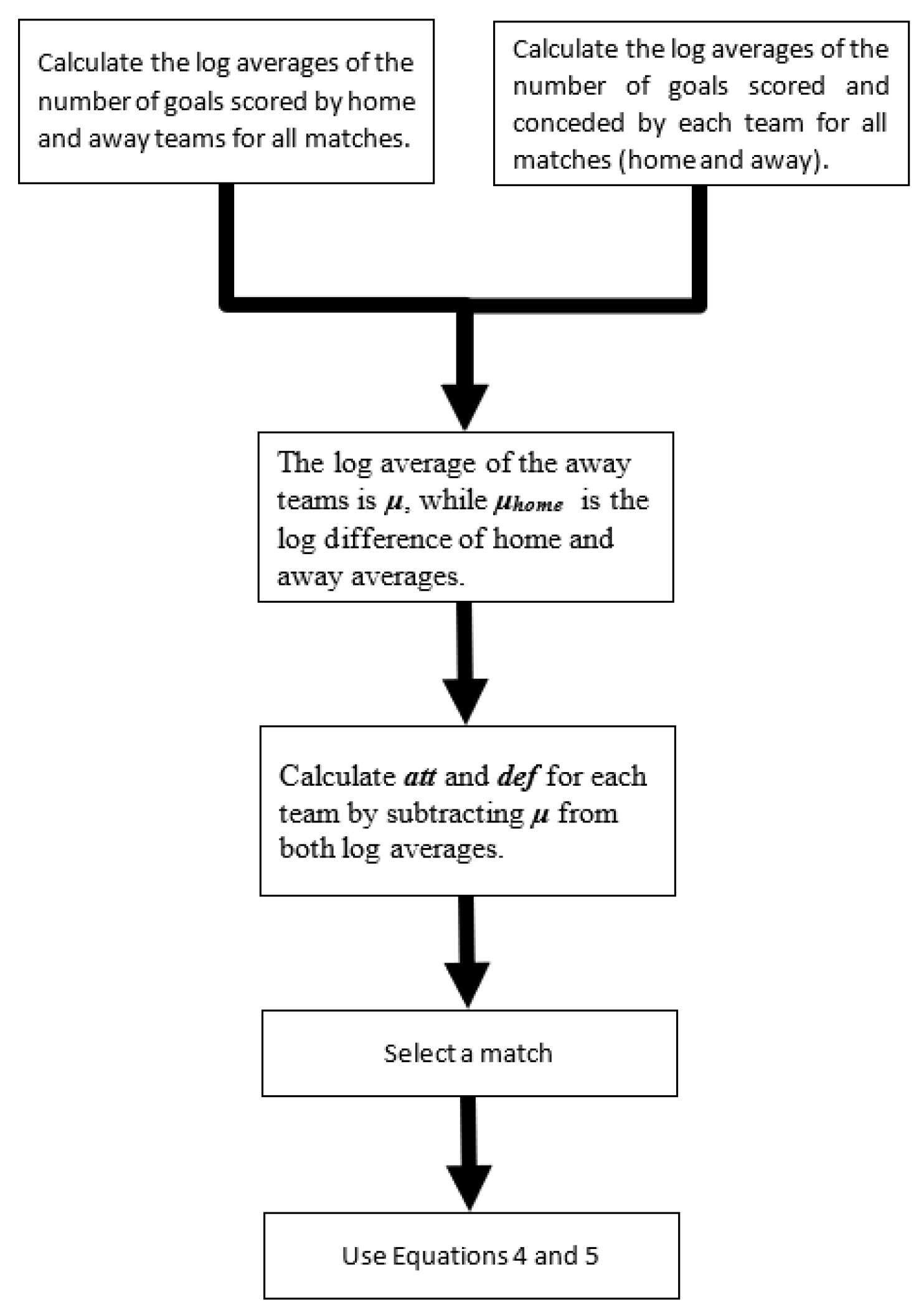
Equations (4) and (5), which are used to calculate the expected number of goals for the home and away team, are Poisson regression models and are considered generalized linear models (GLMs), and thus, we have achieved the modeling of the expected goals for a team using its playing performance. Figure 1 illustrates the steps of our proposed algorithm.
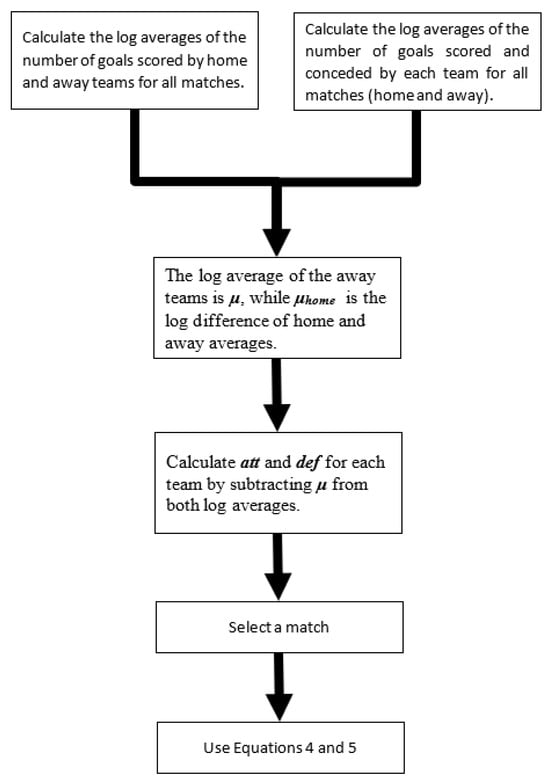
Figure 1.
The steps of our proposed algorithm.
Specifically, these steps are summarized below:
- Calculate the log averages of the number of goals scored by the home and away teams for all matches.
- For each team, calculate the log averages of the number of goals scored and conceded for all the matches (not distinguishing between home and away matches).
- The log average of the away teams is , while is the log difference of home and away averages.
- Calculate att and def for each team by subtracting from both log averages.
The running time of our algorithm is in the number n of the participating teams. We have developed our prototype using the Python programming language version 3.10.
An important aspect of our methodology is the assumption of independence between the goals scored in a match, that is the number of goals scored by the home team does not affect the distribution of the away team’s scores. We discuss this assumption in more detail in the next section.
4. Analysis of the Results
The data for conducting the analysis were retrieved from Kaggle, which include all the necessary information about the matches of the Premier League in the 2022–2023 season.
In the 2022–2023 Premier League’s season, a total of 1084 goals were scored, resulting in a goal average per match. Out of these, 621 were scored by the home sides with an average of goals per match. The remaining 463 goals were scored by the away teams with an average of goals per match. Therefore, home teams score approximately more goals on average compared to the away ones. Manchester City is the team with the most goals in the league followed by Arsenal , while Wolves had the worst attack of the league . Manchester City also had the best defense of the league, conceding 33 goals, which is the same performance as Newcastle.
Almost all teams—except for Everton and Leicester—scored more goals in home matches compared to away ones. Furthermore, all teams, except for Southampton, earned more points from home matches rather than away matches. More specifically, approximately of the total points were earned from home matches and only were earned from away matches. Lastly, out of the 380 total matches, 184 ended with a home win, which is approximately , as depicted in Table 1, compared to only of these matches that finished with an away win. These results, in addition to all the above ones, support the assumption of the methodology: that the home effect is present and should be appropriately quantified in the model.

Table 1.
The 2022–2023 Premier League season: home and away wins.
4.1. Assumption of Independence
We made the assumption that the number of goals scored by the home teams does not affect the distribution of the away teams’ scores. In order to examine whether that assumption is valid, the statistical test was used. Moreover, the cross-tabulation table between the home and away scores for all 380 matches of the 2022–2023 season is illustrated in Table 2, where scores with goals greater than 4 have been grouped as for simplicity.
Table 2.
Home goals’ vs. away goals’ distribution.
Table 3 depicts the results of the test. By taking into account the significance level, which has been set to , and the corresponding p-value, which is , we do not reject the null hypothesis of no relationship between the scores. Consequently, no evidence against the assumption of independence is presented. Thus, in the context of this work, we can assume the independence of the scores.
Table 3.
test results.
4.2. Experimental Results
In Equations (4) and (5), the value of is calculated as the logarithm of the average goals scored in away scores, which is equal to .
The constant for all teams’ home advantage is calculated as the difference of the logarithm of the home and away average goals scored, whose value is , quoted in Table 4.
Table 4.
Results for parameters.
So, a typical away team will score goals, while, on average, a home team is expected to score exp(0.290) = 133% of the goals scored from the away opposition. This result coincides with the observed values, since (average home goals scored) is of .
For the attacking and defensive quality for each team, we will need to calculate the average goals for and the average goals against each team for all the matches played. Table 5 presents those averages along with the attacking and defensive quality for each team.
Table 5.
Attacking (att) and defensive (def) parameters.
A more conservative approach for the calculation of the average goals for and against each team, from which the attacking and defensive parameters are measured, would be to cap match results where, for example, more than 5 goals were scored by a team to 5 (i.e., if a match ended 6-1 to be counted as 5-1). However, following the fact that the number of matches where more than 5 goals were scored by a team is very low (8 in total, and 6 of those refer to 6 goals by a team), no such management was applied as having no material impact on the results.
An indicative example for the calculation of the expected number of goals for each team is presented in Equations (6) and (7). The match selected for the demonstration is Manchester City vs.Liverpool, which was played on 1 April 2023, fixture 29. MC refers to Manchester City and LIV to Liverpool, while xG refers to the expected number of goals that will be scored, utilizing Equations (4) and (5).
The above means that, if Manchester City played Liverpool at home many times, Manchester City would on average score 3.4 goals, while Liverpool would score goals. The observed result of the match was Manchester City vs. Liverpool 4-1.
Furthermore, for this particular match, the probability of the final score being (meaning that Manchester City scores k goals and Liverpool scores h goals), follows a double Poisson distribution and is calculated as follows:
Table 6 presents the probabilities for all scores between the aforementioned teams of the above example using the above formula—the number of goals for home and away matches for each team, which has been capped at nine.
Table 6.
Score probabilities.
For example, the home team—Manchester City—has a probability of to score exactly three goals, while the away team—Liverpool—has a probability of to score exactly one goal. As a result the probability of the final score being 3-1 is (the value in bold in Table 6). The score of 3-1 is also the one with the highest probability of , followed by for a score of 2-1 and for a score of 4-1 (4-1 was the actual result of the match).
Using Table 6, we can also calculate the probability of home win, draw, and away win by taking the sum of the probabilities of that particular outcome. Table 7 illustrates the corresponding probabilities.
Table 7.
Win probabilities—Manchester City vs. Liverpool.
We observed that the probability of a home team win is considerably higher than that of a draw and an away team win, which is in alignment with the fact that Manchester City has the best attacking quality of the league.
In order to test the efficacy of the model, two initial tests were conducted, using all available matches of the season (total of 380) for the parameters estimation present in the model, as per the methodology presented in the previous section.
First, a random 20% sub-sample—i.e., 76 random matches—out of the total of 380 of the 2022–2023 Premier League’s season were randomly selected, and the model estimates were compared against the observed results.
As such, a sample of 76 random matches was created, and for each one, the model estimates were assessed and the difference between the model estimate and observed home and away goals was calculated. It should be noted that the difference between the model estimate and the observed value has been rounded to the nearest integer.
The distribution of differences between model estimates and the observed result for home and away goals for all 76 matches included in the random sub-sample are available in the following tables for home and away scores. As the tables below suggest, the differences range mostly from −2 (meaning the model estimated 2 less goals than actually scored) and 2 (the model estimated 2 goals more than the observed) for both home and away scores; however, a few cases in −3 and 3 were recorded, which mostly refer to unexpected results with a strong favorite side.
For the home scores, of the differences are between −1 and 1, while, in some cases, the model estimated 2 more goals than the actual scores (≈18%). Furthermore, for away scores, the percentage of differences between −1 and 1 rises to more than . That means that most of the scores predicted by the model are either equal to the observed or to a deviation of just one goal. Those results, which are shown in Table 8 and Table 9, are a strong indication that the selected model and methodology are robust and can accurately estimate the goals that a team is likely to score in a match.
Table 8.
Home team goals: model vs. observed.
Table 9.
Away team goals: model vs. observed.
Another examination of the accuracy of the model was conducted by simulating the entire league’s season matches—38 in total, 19 home and 19 away—for a number of teams. The teams selected were Manchester City, Fulham, and Southampton. The rationale behind the selection of those teams was to include teams with different qualities in the league for a more complete view. As such, Manchester City was selected as the champion, which ended the league in the number 1 spot, Fulham with a mid-table finish in league spot number 10, and finally, Southampton, which finished the league at the bottom of the table. For each of those three teams, the estimated goals for the total of 38 matches were calculated, and the aggregated results are available in Table 10. As before, the model results have been rounded to the nearest integer.
Table 10.
Entire league estimated goals simulations.
Following the fact that the above tests were conducted using all the available matches of the season for the calculation of the model parameters, another test was performed in order to have model results on an independent sample, i.e., data that were not used in the model parameters’ estimation. In that regard, in this test, the parameters of the model (, home advantage, att and def parameters for each team) were re-calculated based only on the first round of the league, i.e., the first 19 fixtures, and the matches of the next 5 fixtures were used for prediction accuracy, fixtures 20 to 24, resulting in a total of 50 matches (10 matches per fixture). The decision on selecting only the next five fixtures was reached:
- In order for the calculated parameters to be as relevant as possible, since, as the league progresses, the parameters need updating over time as new results are available, to reflect the overall performance of each team for added precision.
- In order to avoid late fixtures of the league, where many teams have no incentive and many surprise results are present, such as the 0-3 loss of Arsenal at home to Brighton at fixture 36, the loss of Manchester City to Brentford in the late fixtures, or the 4-4 match between Southampton and Liverpool at the last fixture of the league (fixture 38), to name a few.
Regarding the first point above, as hinted, a more optimal methodology would be to re-calculate the parameters in each fixture after each match as the league progresses and try to predict the matches of the next one for maximum precision. In the context of the present analysis and the test below, we made the assumption that, for five games, the parameters can be regarded as relevant and do not need updating.
The results of the 50 matches of the five selected fixtures (20 to 24) as mentioned above are presented in Table 11, where the results have been rounded as in the previous tests.
Table 11.
Differences (model vs. observed) in goals for fixtures 20–24 (50 games in total).
The model does a rather good job in estimating the goals for each team in those 50 matches as the differences were mostly in the range of 0 to 2 goals. Some deviations in the 3-goals difference refer to unanticipated results such as the the 1-1 draw of Manchester City at Nottingham Forest or the 1-0 loss of Manchester City to Tottenham. For both home and way goals, over of the differences range within to 1, indicating that, even on an independent sample, the model performs well in predicting the goals scored by a team.
Considering the above results, the model seemed to perform well in the simulation test. More specifically, for Manchester City, the goal difference between the total goals scored and those estimated by the model was 28 goals (94 to 122 by the model estimate)—where 15 were from home matches (60 observed against 75 estimated by the model) and 13 from the away scores (34 observed against 47 by the model estimate).
For Fulham, a team with a mid-table finish, the model estimate was even closer than that of Manchester City. The model estimated only 20 more total goals compared to the observed (55 versus 75 by the model estimate). From those 20, 11 originated from home scores (31 observed against 42 estimated) and 9 from away (24 observed versus 33 estimated).
Regarding the results for Southampton, the model was even closer for both home and away scores. The model estimated only 9 more goals for home matches (19 observed against 28 by the model estimate), and regarding away scores, the model almost exactly estimated the scores with only a 4-goal difference (17 goals versus the 21 of the model). Overall, the model estimated only 13 more goals for Southampton compared to the actual scores (36 observed versus 49 estimated).
In conclusion, as the above tests indicate, our model performs well in predicting the goals that a team is likely to score in a football match. More specifically, based on the first test, the model was deemed rather successful in estimating the scores of 76 random matches, based on the parameters calculated from all matches available , with differences in goals for both and away teams ranging mostly between and 1. Similar results of satisfactory performance were also observed in predicting the goals of the whole league campaign for the selected teams, as the second test presents. The estimated goals were not so far off the actual goals scored by the teams. Lastly, the results of the final test on an independent sample were also rather good, where the number of estimated goals and the observed ones were very close. Following its general simplicity in terms of application and the good performance of the algorithm, it could be a useful tool for football fans or an initial basis in formulating a betting strategy.
4.3. A Model Weakness
A disadvantage of the model is that it underestimates matches that ended 0-0. This is a common weakness in datasets where the number of zeros is greater than those expected from the Poisson distribution and are called zero-inflated. A football result dataset falls within that above category, following the fact that zero goals scored by a team in a football match is not such an uncommon event. An indication of the above weakness is also evident in the above example where the probability of a 0-0 result of the match between Manchester City and Liverpool is given only a 0.9% probability.
In total, 23 out of 380 matches of the 2022–2023 season ended in 0-0. However, even though the model underestimates all results that ended with no goals, cases where a strong favorite team is present in the match and ended 0-0 are more intensely underestimated.
5. Conclusions and Future Work
In this paper, we investigated whether it is possible to estimate the number of goals scored by a team in a football match based on a team’s past performance. The methodology used assumed that goals scored by a team follow a Poisson distribution, and as a result, the goals scored in a football match follow a double Poisson model—one Poisson distribution for each team. A Poisson regression model was used in order to calculate the expected number of goals for each team using a number of predictors, such as the attacking/defensive quality of the teams and the home team advantage.
Even though the proposed methodology was not complicated and followed a more simplistic form for the score estimation—for example, not accounting for differences in teams from match to match due to injuries, suspensions, and the fact that some teams tend to score more goals against weak opponents and, as such, a model based on goals scored overestimates those teams—the results are rather satisfactory.
More specifically, the model was able to estimate goals scored for each team with good accuracy. The vast majority of differences between the observed number of goals and those estimated by the model are in the range of one goal, and higher deviations occur in results that are considered ‘surprises’, where a strong favorite side was not able to score against a weaker team. On the other hand, a weakness of the model is the strong underestimation of scores that ended with no goals.
As future work, the following could be examined:
- Following the weakness of the model in estimating 0-0 results, an adjustment could be calculated and applied in order to augment the probability of those results estimated by the model, i.e., the use of a zero-inflated Poisson model by estimating a zero-inflation parameter in order to increase the number of zeroes estimated by the model.
- The most recent results of a team may be more representative of the estimation of the goals of that team in a future match than older ones, a fact that was not taken into account in the present study. As such, an adjustment could be performed in the model in order to reflect that fact (i.e., a weighting factor could be calculated in order for the recent games to be more impactful on the estimation results).
- Consider the fact that certain teams in the late fixtures and towards the end of the season have no interest, since they cannot achieve anything better in the remaining fixtures. For example, they are several points away from the fourth place, which leads to the UEFA Champions League, but those points cannot be obtained with the remaining matches. In those cases, the results are not completely representative of the team’s performance. This fact can impact the performance of a team in both ways: either playing worse due to the lack of an incentive or playing well, since there is no pressure for the result. The latter is especially true for young players.
- Check the performance of the model in non-national leagues, where the number of historical matches is not as high as national leagues. An example of this could be to use information from the UEFA Champions League’s results, where each team plays considerably lower matches compared to their national league.
Author Contributions
Conceptualization, K.L.; Software, K.L.; Formal analysis, D.K.; Investigation, K.L.; Writing—original draft, K.L.; Writing—review & editing, D.K., G.F. and V.S.V. All authors have read and agreed to the published version of the manuscript.
Funding
This research received no external funding.
Institutional Review Board Statement
Not applicable.
Informed Consent Statement
Not applicable.
Data Availability Statement
The original contributions presented in the study are included in the article, further inquiries can be directed to the corresponding author.
Conflicts of Interest
The authors declare no conflicts of interest.
References
- Lee, A.J. Modeling scores in the Premier League: Is Manchester United really the best? Chance 1997, 10, 15–19. [Google Scholar] [CrossRef]
- Maher, M.J. Modelling association football scores. Statist. Neerland. 1982, 36, 109–118. [Google Scholar] [CrossRef]
- Karlis, D.; Ntzoufras, I. On modeling Soccer Data. Student 2000, 3, 229–244. [Google Scholar]
- Karlis, D.; Ntzoufras, I. Analysis of sports data by using bivariate Poisson models. J. R. Stat. Soc. Ser. D (Stat.) 2003, 52, 381–393. [Google Scholar] [CrossRef]
- Dixon, M.J.; Robinson, M.E. A birth process model for association football matches. J. R. Stat. Soc. Ser. D (Stat.) 1998, 47, 523–538. [Google Scholar] [CrossRef]
- Karlis, D.; Ntzoufras, I. Statistical modeling for soccer games: The Greek League. In Proceedings of the Fourth Hellenic-European Conference on Computer Mathematics and Its Applications, Athens, Greece, 24–26 September 1998; Lipitakis, E.A., Ed.; LEA: Athens, Greece, 1998; pp. 541–548. [Google Scholar]
- Dixon, M.J.; Coles, S.G. Modelling association football scores and inefficiencies in the football betting market. J. R. Stat. Soc. Appl. Stat. 1997, 46, 265–280. [Google Scholar] [CrossRef]
- Rue, H.; Salvesen, Ø. Prediction and retrospective analysis of soccer matches in a league. J. R. Stat. Soc. Ser. D (Stat.) 2000, 49, 399–418. [Google Scholar] [CrossRef]
- Penn, M.; Donnelly, C.A. Analysis of a double Poisson model for predicting football results in Euro 2020. PLoS ONE 2022, 17, e0268511. [Google Scholar] [CrossRef] [PubMed]
Disclaimer/Publisher’s Note: The statements, opinions and data contained in all publications are solely those of the individual author(s) and contributor(s) and not of MDPI and/or the editor(s). MDPI and/or the editor(s) disclaim responsibility for any injury to people or property resulting from any ideas, methods, instructions or products referred to in the content. |
© 2024 by the authors. Licensee MDPI, Basel, Switzerland. This article is an open access article distributed under the terms and conditions of the Creative Commons Attribution (CC BY) license (https://creativecommons.org/licenses/by/4.0/).