Article

Studies of Fluorescence Lifetimes of Biological Warfare Agents Simulants and Interferers Using the Stroboscopic Method

by
Miron Kaliszewski
1,
Mirosław Kwaśny
1,
Aneta Bombalska
1,*,
Maksymilian Włodarski
1,
Elżbieta Anna Trafny
2 and
Krzysztof Kopczyński
1
1
Institute of Optoelectronics, Military University of Technology, Kaliskiego 2, 00-908 Warsaw, Poland
2
Biomedical Engineering Centre, Institute of Optoelectronics, Military University of Technology, Kaliskiego 2, 00-908 Warsaw, Poland
*
Author to whom correspondence should be addressed.
Appl. Sci. 2024, 14(16), 7332; https://doi.org/10.3390/app14167332
Submission received: 26 June 2024 / Revised: 14 August 2024 / Accepted: 16 August 2024 / Published: 20 August 2024

Abstract

:
The fluorescence decays (FDs) of 27 dried vegetative bacteria, bacterial endospores, fungi, and pollens were measured and determined using a stroboscopic technique. Pulsed nanosecond LED sources, emitting light at wavelengths of 280, 340, and 460 nm, were used for the excitation of biological samples. The implicit advantages of the stroboscopic method are high sensitivity, speed of a single measurement (10–60 s), miniaturization of the device, and relatively low price compared to the typical lifetime methods. The Principal Component Analysis (PCA) method was used for chemometric analysis. It was found that the excitation at 340, 460, and data merged from 340 and 460 nm effectively separate individual groups of biological substances. These findings provide evidence that fluorescence decay data may allow the classification of the biological samples, and the FDs measurement method can be complementary to the study of fluorescence spectra.

1. Introduction

The term “bio-aerosol” is used to describe various substances: microorganisms and their fragments, toxins, and particles originating from the decay of various living organisms. Bio-aerosol may contain live bacteria and their spores, viruses, fungi, leaf fragments, pollen, cellulose, humic and fulvic acids, chlorophyll, and dust [1]. In addition, aromatic hydrocarbons from industrial and engine exhaust appear in the air. We inhale and exhale air containing many such particles, which may affect human health [2,3].
Air monitoring has become an important element of civil protection. In addition to civilian applications for testing air purity in workspaces, public utilities, and residents, an early warning system against a potential bioterrorist activity is used. Of the thousands of bacteria, only a small percentage cause infection and disease [4]. However, only 45 are considered by CDC as potential bio-weapons [5].
The laser-induced fluorescence (LIF) method is used to build sensitive analyzers of biological agents in both civilian and military applications. This method is used for the detection and classification of biological material in water [6], in the air [7,8,9,10,11,12,13], and on the surface [14,15,16]. Fluorescence is the most sensitive spectroscopic method, and it has been used in many fields of research, including medicine [17,18,19]. The LIF methods are mainly based on the analysis of one or two emission bands. It has been shown that the fluorescence of a single particle excited with more than one wavelength can strongly improve the classification of bio-aerosols due to the involvement of emission from various fluorophores. The fluorescence spectra do not provide sufficient information for clear and reliable identification of air-borne species but allow rough, real-time discrimination of naturally or intentionally released biological warfare agents from interferents [20,21,22].
An important parameter of fluorescence, apart from spectra, is the fluorescence lifetime. Steady-state fluorescence spectra indicate that the emission phenomenon occurs at specific wavelengths of radiation, while the fluorescence lifetime indicates how this phenomenon occurs. The fluorescence lifetime of bio-fluorophores is very sensitive to their microenvironment in the protein and makes it possible to discriminate between different biological molecules.
The research aims to conduct a systematic study to create a lifetime domain database of dry biological samples for real-time detection and monitoring systems. Some reports on the time-resolved fluorescence of microorganisms were published. Usually, one or two decay time models have been applied to describe the decay kinetics of the samples [23,24,25,26]. James and Siemiarczuk used a stroboscopic technique for fluorescence decay analysis of albumin and found at least three lifetime components [27].
This article presents the basics of the method, the construction of the equipment, and techniques used for the measurement of fluorescence lifetimes. The aim of the current work was to determine a database of fluorescence lifetimes of biological substances that are simulants and interferents of biological warfare agents (BWAs). In addition to vegetative bacteria, their spore forms, plant pollen and fungi, and commercial bioinsecticides used in agriculture were also examined. At the Institute of Optoelectronics (IOE), many devices for BWA detection have been developed and implemented [13,28], including fluorescence lidars [9]. The developed database is the basis for the IOE engineers to build more advanced LIF analyzers based on a combination of spectra and fluorescence lifetime measurements, which allows improved classification selectivity.
A common, recommended method for testing lifetimes is Time-Correlated Single Photon Counting (TCSPC) [29]. For the analysis of small concentrations of biological substances, the method has many limitations. The measurement might take many hours, which, in the case of fluorescence excitation with UV radiation, often means photochemical decomposition of the substance or significant changes in its lifetime. Therefore, other fast and sensitive methods are being sought. These include, among others, the stroboscopic method. In the article [13], we showed an example of its use in the analysis of suspensions of several bacteria.
The stroboscopic method was introduced to the market in 1990 and allows the measurement of the fluorescence lifetime of bacteria and its biological interferents [14]. Its main advantage is high sensitivity and the short time of a single measurement at 10–60 s. The name characterizes the measurement method, which examines the fluorescence intensity in very short (relative to the fluorescence decay time) moments in time synchronized with the moment of excitation. The great advantage of the stroboscopic technique is its relatively low cost and high sensitivity, allowing measurement of low fluorescence signals. The classic method, Time-Correlated Single Photon Counting (TCSPC), is burdened by very long measurement times, up to several hours, and during the irradiation, the biological sample can be degraded.
Rapid progress in semiconductor technologies allowed the development and miniaturization of bio-analytical systems based on UV LED. For that reason, it is important to test the new light sources for their potential capabilities for the future development of new generations of detectors [30,31,32].
While the literature research concerning the fluorescence lifetimes of bacteria, spores, fungi, and pollens is broad, the data are strongly fragmented, and there is a lack of reliable comparison between different species. Moreover, experiments are conducted in different conditions, which makes them inconsistent. In our research, we examined 27 substances of biological origin under controlled and identical parameters. We believe that this approach will improve the comparability among the studies.
Bacteria, bacterial spores, fungi, pollens, and tissue are a combination of thousands of compounds. A number of them are fluorescent, which makes them suitable for investigation using UV sources. The main source of endogenous fluorescence in cells and biological tissues are aromatic amino acids used to build proteins. Of the 20 amino acids that are basic units of proteins, only tryptophan (Trp), tyrosine (Tyr), and phenylalanine (Phe) fluoresce under UV excitation [33]. Among these amino acids, tryptophan exhibits the strongest fluorescence with excitation and emission maxima of about 280 and 340 nm, respectively. In contrast, phenylalanine fluorescence is very short, and tyrosine fluorescence is usually quenched due to interactions with other protein chains [34]. Both the spectral shift and the fluorescence lifetime of tryptophan are highly sensitive to the ligand they are bound to, as well as to the polarity of the microenvironment of their occurrence [35,36].
While the fluorescence of proteins and amino acids is an indicator of the presence of biological material, the fluorescence of metabolic mediators such as reduced forms of nicotinamide adenine dinucleotide (NADH) and its phosphorylated form, NAD(P)H, flavin dinucleotide adenine (FAD) is considered an indicator of the activity of a microorganism. The maxima of excitation and emission of both NADH and NAD(P)H are about 350 and 450 nm, respectively. The free, unbounded NADH has about 0.4 ns lifetime, while bounded proteins present a lifetime of about 2–3 ns. The oxidized form NAD+ is non-fluorescent. The fluorescence lifetime of free and protein-bound FAD is less than 0.1 and 2.3–2.9 ns, respectively [33,37,38,39,40].
Table 1 contains the absorption and emission parameters of selected compounds contributing to the fluorescence of biological systems.
The current work concerns the analysis of dry samples of bacteria and their interferents (fungi, pollens), i.e., real situations with air pollution and contamination with biological materials. In addition to determining the fluorescence lifetimes, data analysis was carried out using PCA.

2. Materials and Methods

2.1. Measurement Setups

The measurements were performed using steady-state and lifetime fluorimeters:
(a) Fluorimeter FS 900 (Edinburgh Instr., Livingston, Scotland) allowing the measurement of excitation–emission matrices (EX-EMs);
(b) EasyLife System (Photon Technology International, Birmingham, NJ, USA) with LED excitation of 280, 340, and 460 nm for fluorescence measurements of suspensions and solid particles (Figure 1). Fluorescence excitation was performed using nanosecond pulse LEDs.

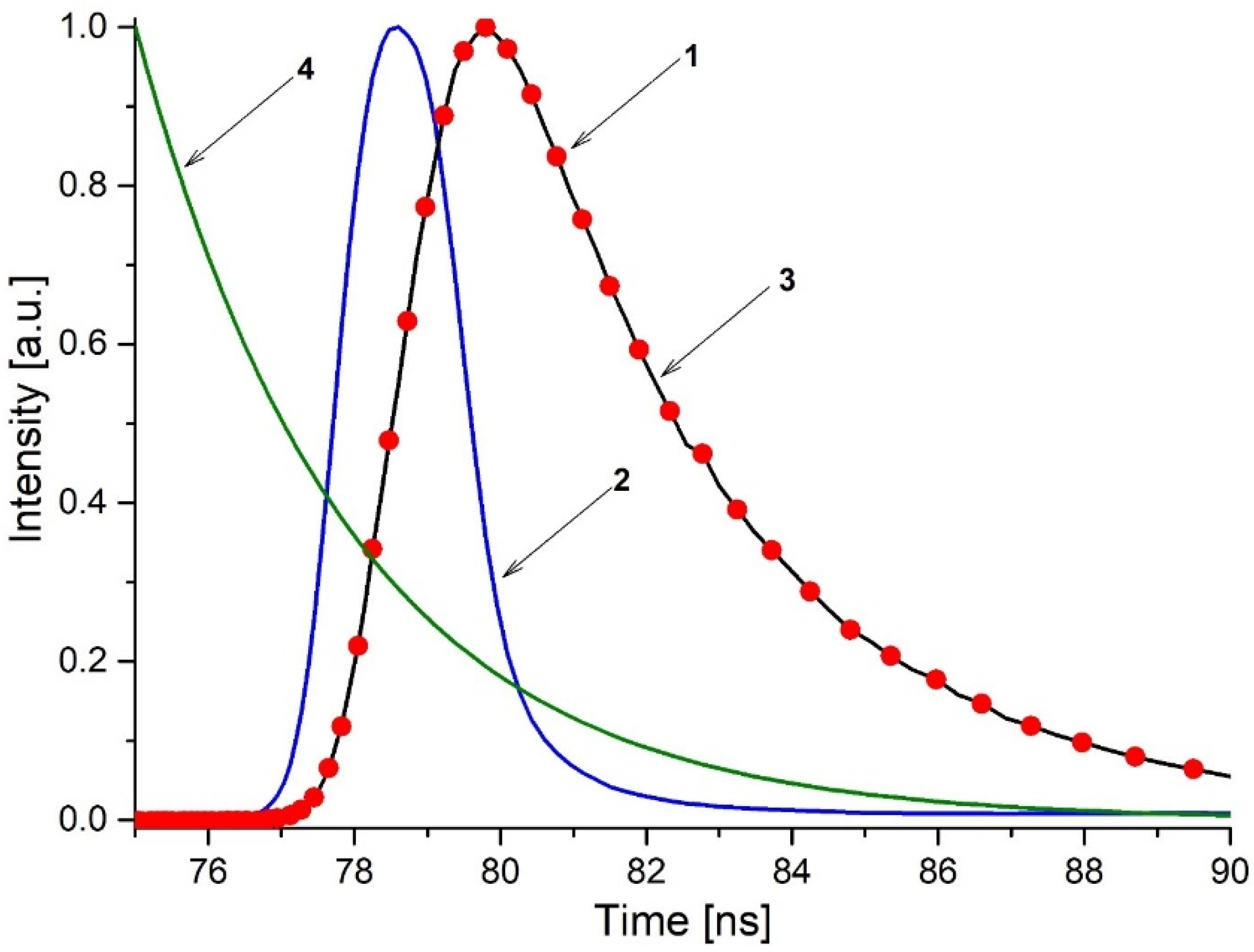
2.2. Fluorescence Lifetime Measurements

Fluorescence decays of biological samples were measured using a stroboscopic technique using the EasyLife LS system. Three LED modules generating radiation with wavelengths 280 nm, 340 nm, and 460 nm of nanosecond pulses were used for sample excitation. Wide spectral characteristics of diodes were corrected with bandpass filters (Semrock, Rochester, NY, USA) FF-280/20, FF-340/26, and FF-447/60, respectively. Long-pass filters for cutting off excitation bands on the emission path were used as follows: FF-300LP, LP-355, and F514R for 280 nm, 340 nm, and 460 nm excitation, respectively. Measurements were carried out at room temperature, and all decay data were recorded using 10 averages to obtain a smooth decay curve. Solid samples were fixed with an aluminum holder with a Suprasil quartz window. The holder allowed the collection of the fluorescence signal from the surface of the sample. The averages of fluorescence lifetimes were calculated using Formula (1):
τav = (∑(ai τi)/(∑ai)
where τi is the fluorescence lifetimes of various fluorescent forms and ai is the corresponding pre-exponential factors.

2.3. Data Analysis

The fluorescence lifetimes were estimated using Felix32 (version 1.10) software dedicated to an EasyLife fluorimeter. For the deconvolution of the sample, the decay signal from the excitation pulse was corrected using the instrument response function (IRF), which was measured using dry Syloid. This compound does not exhibit fluorescence.
A fluorescence decay D(t) of a single fluorophore in a homogeneous solution can usually be described as a single-exponential function (2):
D(t) = aexp(−t/τ)
where τ is the fluorescence lifetime and a is the pre-exponential factor.
If the sample contains more than one fluorophore or its environment is heterogeneous, the fluorescence decay is described as a sum of exponential functions:
D(t) = ∑_(i = 1)^n[a_i exp](−t/τi)
where τi is the fluorescence lifetimes of various fluorescent forms and ai is the corresponding pre-exponential factors [48].
The decay curves described by Equations (2) and (3) will only be observed if the sample is excited by an infinitely narrow pulse. Usually, the excitation pulse width affects the observed decay Dobs(t). Therefore, deconvolution, using instrument response function (IRF) L(t), is necessary (4) [48]:
Dobs (t) = ∫_0^t L(t − s)D(s)ds
Figure 2 shows an example of the traces obtained in a typical fluorescence experiment.
Once the Dobs(t) and L(t) have been measured, the analysis software performs iterative reconvolution according to Equation (4), varying the fit parameter ai and ti until the best fit to the experimental decay is obtained [49].
For statistical analysis, the Principal Component Analysis (PCA) was performed with the SIMCA-P program from Umetrics AB, Umea, Sweden. The data analyzed were mean-centered and scaled to the unit variance.

2.4. Microorganisms

The reference materials used throughout this study (Table 1) were prepared by the Military Institute of Hygiene and Epidemiology (MIHE) in Warsaw.
The preparation procedure of bacterial spores, vegetative bacteria, and fungi, including lyophilizes, was as follows: Vegetative cells of five Bacillus strains and Escherichia coli and Micrococcus luteus were used. The working cultures of these strains were prepared from the reference stock and were grown on the appropriate liquid media for 18 h at 37 °C. The endospores were stored in 50% ethyl alcohol at a temperature of 4 °C. Endospores in ethyl alcohol or a suspension of endospores prepared in sterile deionized water (SDW) were used for experiments. Candida albicans and four strains of filamentous fungi were also used. The Candida albicans strain was grown in a liquid YPD medium, and filamentous fungi were cultured in an MEA medium. The samples of fungi used in experiments were suspended in sterile saline.
Bacterial lyophilizates obtained from BG endospores and Micrococcus luteus or Penicillium chrysogenum vegetative cells were used in this study. BG strain ATCC 9372 was grown on a solid 2 SG endosporulation medium. BG endospores suspended in SDW and M. luteus or P. chrysogenum cells suspended in sterile saline solution were freeze-dried in a Lyovac GT2 (Leybold GmbH, Cologne, Germany) at maximum vacuum 6 × 10⁻¹ mbar for 24 h. Before each experiment, the bacterial lyophilizates were placed in a glove box (Model 830-ABB/Spz800-HEPA/D, Plas-Labs, Inc., Lansing, MI, USA). The bacterial lyophilizates were then scraped from the bottom of the flasks using a 28 cm Cell Scraper (Greiner Bio-One GmbH, Kremsmünster, Austria) and were hand-crushed in mortars. Small amounts of biological material were placed on the surface of the aluminum holder and covered with a Suprasil quartz plate. The sample list and abbreviations used in the article are shown in Table 2.
Technical spores were prepared in order to simulate data also in field conditions. Their composition, as in the case of possible BWs, includes auxiliary substances that stabilize the aerosol.

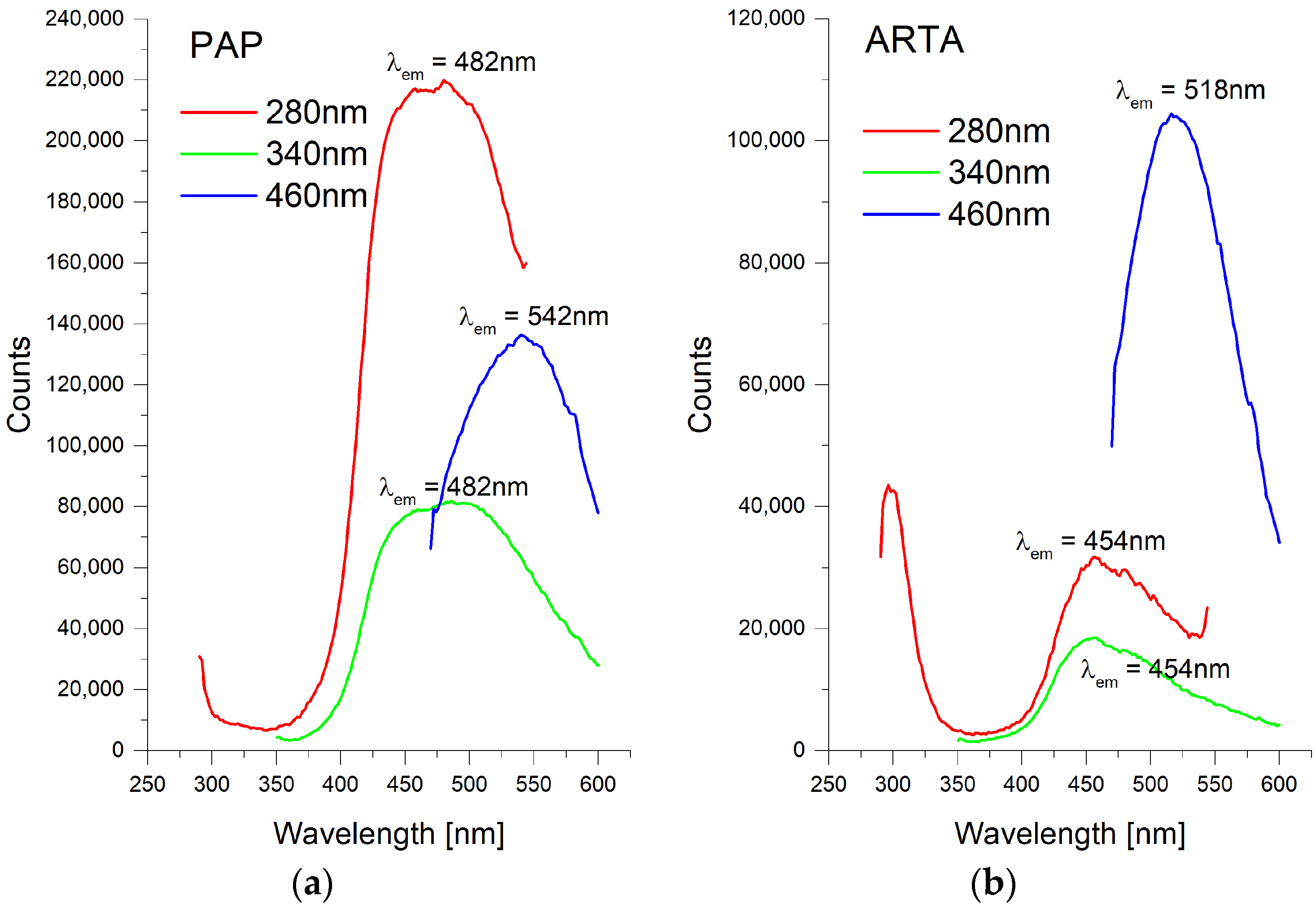
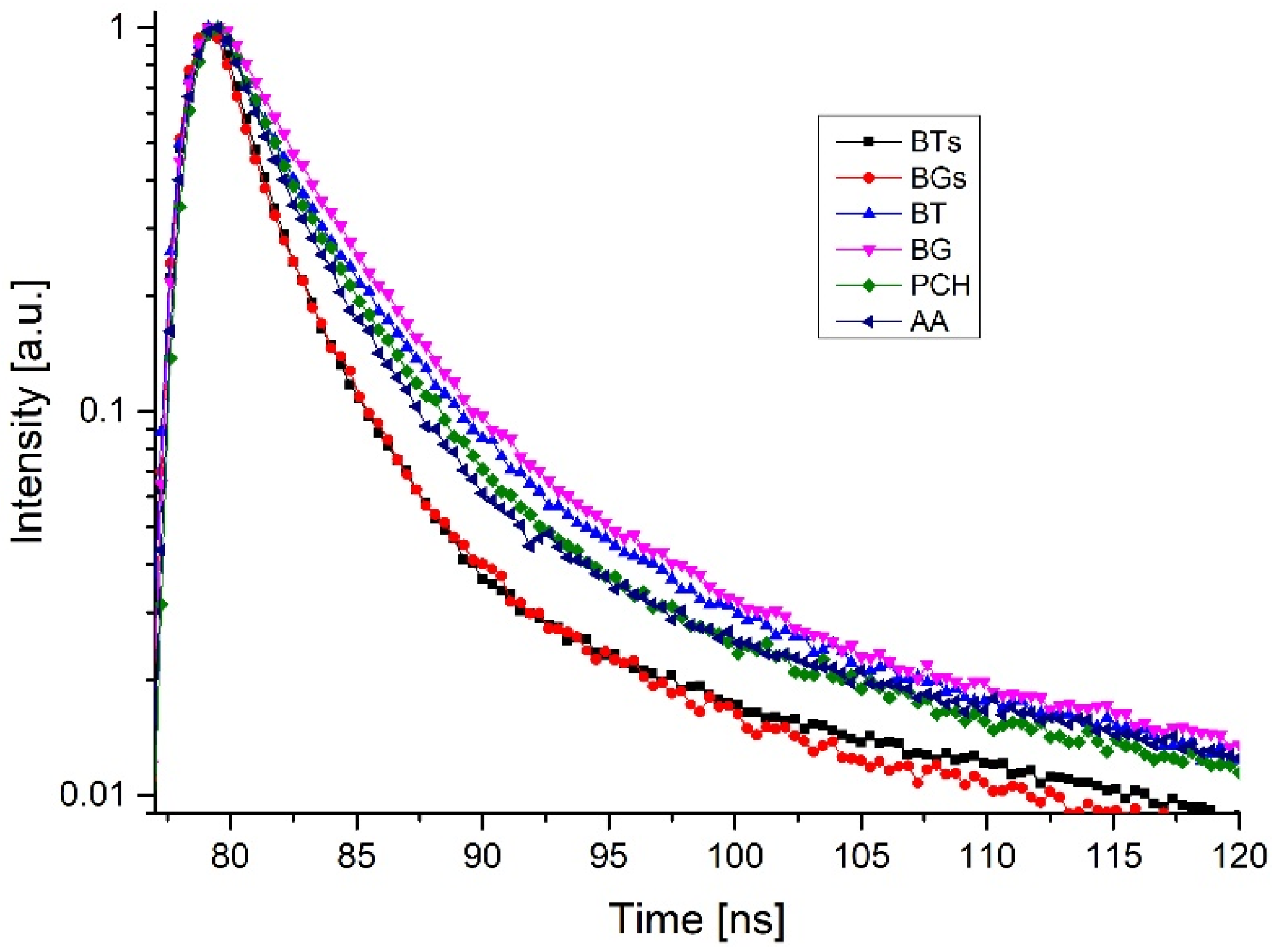
3. Results and Discussion

The main absorption bands of materials of biological origin, such as living bacteria, spores, and fungi, occur around 280 and 340 nm. They cover a wide range of excitation and emission, including protein and NADH bands. The pollens additionally display a strong band allowing excitation in visible blue light ranging from 400 nm to 470 nm. Examples of emission characteristics of plant pollens excited with 280, 340, and 460 nm, respectively, are shown in Figure 3.
Therefore, the use of 460 nm excitation can improve the discrimination of pollens from other species. The excitation and emission peaks at 460 nm and 520 nm, respectively, are attributed to the carotenoids that are present in pollens.
Emission spectra of aqueous solutions/suspensions of biological agents differ from those of dehydrated ones, as shown in the example of pure tryptophan (Figure 4).
Additional emission modes are generated in the solid phase, and therefore, decay measurements are also possible for fluorescence excitation at 460 nm. The fluorescence lifetime data of the samples analyzed are presented in Table S1 in Supplementary Materials.
Each group exhibited its best fit when using a three-component equation at an excitation of 280 nm. The three-exponential fit was observed for pollens at each examined excitation wavelength, which was also reported by O’Connor et al. [50].
Several vegetative bacteria (EC—excited at 280 nm; BC, BS, ML, PA—excited at 340 nm; and BG, BS, BT—excited at 460 nm) showed two- or three-component fluorescence lifetimes reaching the same or similar Chi2 values.
Due to the complex composition of biological samples, at least two-component fitting produces satisfactory results. Awad et al. [51] also obtained a three-exponential decay for pathogenic bacteria, although they calculated lifetimes about two times shorter for fast and intermediate components.
Figure 5 shows fluorescence decays obtained at 280 nm excitation. The bacterial endospores presented more rapid decay than the vegetative bacteria and fungi.
A comparison of the ranges of average fluorescence lifetime of the analyzed substances at excitations of 280, 340, and 460 nm is shown in Figure 6.
Figure 6 shows that the smallest variation in average fluorescence lifetimes occurs in the case of excitation at a wavelength of 280 nm. This is understandable because proteins responsible for this excitation consist, among others, of three fluorescent amino acids, of which the fluorescence of phenylalanine can be neglected, and tryptophan and tyrosine have similar emission decay times.
However, the excitation wavelength at about 280 nm is universal for all biological materials and is often used in early BWA detection devices. It should be emphasized that the analysis of fluorescence decay characteristics at this excitation wavelength should be used to detect the presence of biological agents and not to classify them. Excitation wavelengths at 340 and 460 nm are more usable for classification purposes. Lifetimes of vegetative bacteria, pollen, and spores are best separated at 340 nm excitation, while fungi are clearly distinguished at 460 nm. This is primarily due to the large variety of different fluorophores, excited at these wavelengths, contained in these materials.
The averaged parameter represents the relationship between the samples more uniformly when compared to the two or three lifetime components. It appears that at each excitation wavelength, the pollens display the shortest mean lifetimes, while the fungi display the longest. It can be concluded that fluorescence lifetimes vary from group to group depending on the excitation wavelength. Those differences suggest that fluorescence decay times could potentially be used to distinguish between various groups of microorganisms. However, the lifetimes and the number of components can vary depending on the fitting procedure, which points to quite an arbitrary character of lifetime data analysis. The results can also depend on excitation and emission wavelength [26,52].
It can be observed that pollens display shorter lifetimes than other considered groups. The first two components exhibit a lifetime of 1–2 ns at each of the excitation wavelengths. However, at 280 nm and 460 nm, the percentage contributions of the first and the second components are similar. The third component displays a short lifetime value at excitation at 280 nm, whereas at 340 and 460 nm excitation wavelengths, it was shifted to longer times around 6–7 ns. The contribution of the third lifetime component at each excitation wavelength is relatively constant and reaches about 10%. The bacterial spores are characterized by a 90% contribution (0.5–1.5 ns) for the first component at all excitation wavelengths examined. This is a significant feature as compared to other biological materials due to the absence of the third component for 340 nm and 460 nm excitation. Fungi display a relatively long lifetime at all examined excitation wavelengths, and individual results are rather diverse, especially at 340 nm and 460 nm excitation. An example of the percentage of individual fluorescence decay times for 340 nm excitation is shown in Figure 7.
The difficulties in FD time comparison can be avoided by a different analytical approach—Principal Component Analysis (PCA). This allows results to be obtained that are reliable and independent of the operator.
It has been demonstrated that clustering methods in spectroscopy are suitable for the classification of biological material. The great advantage of PCA is its ability to produce real-time data analysis based on the spectral characteristics of the sample [28,53]. Additionally, results are independent of the curve fitting procedure.
The PCA score plots of fluorescence decays of four groups of biological samples are shown in Figure 8 and Figure 9. All variants of single-, double-, and triple-wavelength excitation data were also examined. The decay data obtained at 280 nm did not produce satisfactory discrimination of any group of biological samples. It may be due to relatively similar fluorescence decay patterns of proteins that are ubiquitous in all biological samples. More effective discrimination occurs for 340 nm excitation because the vegetative bacteria could be noticeably distinguished from other groups (Figure 8). The 460 nm excitation delivers a clear distinction of bacterial spores from other groups (Figure 9).
Using 340 and 460 nm wavelengths (Figure 10) for joined decay data in the PCA yielded slightly better classification results compared to the merged three wavelengths’ data. This suggests that the additional information at 280 nm may not be informative for differentiating the biological samples within this specific context. Fungi are characterized by the greatest differences in the composition of fluorophores; hence, they are located in a large range of positions on the PCA chart.

4. Conclusions

The results presented show the potential for discrimination between the species examined. Two different approaches were compared for biological sample classification based on their fluorescence decays. The first one applied fluorescence lifetimes, which were determined using a fitting procedure. The second one employed PCA of decay curves data. The PCA method allowed sample classification using a combination of multiple excitation wavelengths. The 280 nm excitation did not produce satisfactory discrimination. The best results were obtained for the combination of the 340 nm and 460 nm excitations. The data presented above were completed using a low-power LED, although laser diodes available on the market can be successfully applied in low-cost single particle detectors using fluorescence decay measurements. The results and an approach to the data analysis using PCA show the possibility of the development of an environmental sensor for fast and reliable discrimination of biological samples.
In the article [13], we presented the results of PCA analysis of the same materials based on the designated EX-EM matrices. To obtain such a matrix, approximately 30 spectra with different excitations must be performed, which takes over 30 min, and much higher concentrations of the substance are required. In the stroboscopic method, it is enough to determine the lifetime with excitation of 340 nm (or 280, 340, and 460 nm) to achieve the same result. The stroboscopic method with excitation by the above-mentioned sources is universal for practically all fluorescent compounds because it is difficult to find substances with absorption bands outside the range of the above-mentioned wavelengths. In addition to its simplicity, the stroboscopic method is characterized by high speed, precision (the measurement can be repeated many times to increase the signal/noise ratio), and an accuracy of up to 0.1 ns. The results of the lifetimes of fluorescence patterns showing mono-exponential decay, such as NATA and NADH, perfectly match the data obtained using other methods.

Supplementary Materials

The following supporting information can be downloaded at https://www.mdpi.com/article/10.3390/app14167332/s1, Table S1: Fluorescence lifetime values and their contribution calculated for dry microorganisms for 280 nm, 340 nm, and 460 nm excitation.

Author Contributions

Conceptualization, M.K. (Mirosław Kwaśny), M.K. (Miron Kaliszewski) and M.W.; methodology, M.K. (Miron Kaliszewski), M.W. and M.K. (Mirosław Kwaśny); formal analysis, M.K. (Mirosław Kwaśny) and M.K. (Miron Kaliszewski); investigation, M.K. (Miron Kaliszewski), M.W., A.B. and E.A.T.; data curation, M.K. (Miron Kaliszewski); writing—original draft preparation, M.K. (Miron Kaliszewski) and M.K. (Mirosław Kwaśny); writing—review and editing, M.K. (Miron Kaliszewski) and A.B.; visualization, M.K. (Miron Kaliszewski), M.W. and M.K. (Mirosław Kwaśny); supervision, M.K. (Miron Kaliszewski), K.K. and M.K. (Miron Kaliszewski); project administration, M.K. (Miron Kaliszewski) and M.K. (Mirosław Kwaśny); funding acquisition, M.K. (Mirosław Kwaśny). All authors have read and agreed to the published version of the manuscript.

Funding

This work was supported by The National Centre for Research and Development grant NO. “O N507 418840”.

Institutional Review Board Statement

Not applicable.

Informed Consent Statement

Not applicable.

Data Availability Statement

On request.

Conflicts of Interest

The authors declare no conflicts of interest.

References

  1. Després, V.R.; Alex Huffman, J.; Burrows, S.M.; Hoose, C.; Safatov, A.S.; Buryak, G.; Fröhlich-Nowoisky, J.; Elbert, W.; Andreae, M.O.; Pöschl, U.; et al. Primary biological aerosol particles in the atmosphere: A review. Tellus Ser. B Chem. Phys. Meteorol. 2012, 64, 15598. [Google Scholar] [CrossRef]
  2. Blais-Lecours, P.; Perrott, P.; Duchaine, C. Non-culturable bioaerosols in indoor settings: Impact on health and molecular approaches for detection. Atmos. Environ. 2015, 110, 45–53. [Google Scholar] [CrossRef] [PubMed]
  3. Fröhlich-Nowoisky, J.; Kampf, C.J.; Weber, B.; Huffman, J.A.; Pöhlker, C.; Andreae, M.O.; Lang-Yona, N.; Burrows, S.M.; Gunthe, S.S.; Elbert, W.; et al. Bioaerosols in the Earth system: Climate, health, and ecosystem interactions. Atmos. Res. 2016, 182, 346–376. [Google Scholar] [CrossRef]
  4. Doron, S.; Gorbach, S.L. Bacterial Infections: Overview. Int. Encycl. Public Health 2008, 273–282. [Google Scholar] [CrossRef]
  5. CDC. Bioterrorism Agents/Diseases. Available online: https://emergency.cdc.gov/agent/agentlist-category.asp (accessed on 22 December 2023).
  6. Gabbarini, V.; Rossi, R.; Ciparisse, J.F.; Malizia, A.; Divizia, A.; De Filippis, P.; Anselmi, M.; Carestia, M.; Palombi, L.; Divizia, M.; et al. Laser-induced fluorescence (LIF) as a smart method for fast environmental virological analyses: Validation on Picornaviruses. Sci. Rep. 2019, 9, 12598. [Google Scholar] [CrossRef]
  7. Savage, N.J.; Krentz, C.E.; Könemann, T.; Han, T.T.; Mainelis, G.; Pöhlker, C.; Alex Huffman, J. Systematic characterization and fluorescence threshold strategies for the wideband integrated bioaerosol sensor (WIBS) using size-resolved biological and interfering particles. Atmos. Meas. Tech. 2017, 10, 4279–4302. [Google Scholar] [CrossRef]
  8. Huffman, J.A.; Treutlein, B.; Pöschl, U. Fluorescent biological aerosol particle concentrations and size distributions measured with an Ultraviolet Aerodynamic Particle Sizer (UV-APS) in Central Europe. Atmos. Chem. Phys. 2010, 10, 3215–3233. [Google Scholar] [CrossRef]
  9. Wojtanowski, J.; Zygmunt, M.; Muzal, M.; Knysak, P.; Młodzianko, A.; Gawlikowski, A.; Drozd, T.; Kopczyński, K.; Mierczyk, Z.; Kaszczuk, M.; et al. Performance verification of a LIF-LIDAR technique for stand-off detection and classification of biological agents. Opt. Laser Technol. 2015, 67, 25–32. [Google Scholar] [CrossRef]
  10. Hernandez, M.; Perring, A.E.; McCabe, K.; Kok, G.; Granger, G.; Baumgardner, D. Chamber catalogues of optical and fluorescent signatures distinguish bioaerosol classes. Atmos. Meas. Tech. 2016, 9, 3283–3292. [Google Scholar] [CrossRef]
  11. Duschek, F.; Fellner, L.; Gebert, F.; Grünewald, K.; Köhntopp, A.; Kraus, M.; Mahnke, P.; Pargmann, C.; Tomaso, H.; Walter, A. Standoff detection and classification of bacteria by multispectral laser-induced fluorescence. Adv. Opt. Technol. 2017, 6, 75–83. [Google Scholar] [CrossRef]
  12. Taketani, F.; Kanaya, Y.; Nakamura, T.; Koizumi, K.; Moteki, N.; Takegawa, N. Measurement of fluorescence spectra from atmospheric single submicron particle using laser-induced fluorescence technique. J. Aerosol Sci. 2013, 58, 1–8. [Google Scholar] [CrossRef]
  13. Kwaśny, M.; Bombalska, A.; Kaliszewski, M.; Włodarski, M.; Kopczyński, K. Fluorescence Methods for the Detection of Bioaerosols in Their Civil and Military Applications. Sensors 2023, 23, 3339. [Google Scholar] [CrossRef] [PubMed]
  14. Włodarski, M.; Kaliszewski, M.; Trafny, E.A.; Szpakowska, M.; Lewandowski, R.; Bombalska, A.; Kwaśny, M.; Kopczyński, K.; Mularczyk-Oliwa, M. Fast, reagentless and reliable screening of “white powders” during the bioterrorism hoaxes. Forensic Sci. Int. 2015, 248, 71–77. [Google Scholar] [CrossRef]
  15. Trafny, E.A.; Lewandowski, R.; Stȩpińska, M.; Kaliszewski, M. Biological threat detection in the air and on the surface: How to define the risk. Arch. Immunol. Ther. Exp. 2014, 62, 253–261. [Google Scholar] [CrossRef] [PubMed]
  16. Babichenko, S.; Bentahir, M.; Piette, A.S.; Poryvkina, L.; Rebane, O.; Smits, B.; Sobolev, I.; Soboleva, N.; Gala, J.L. Non-Contact, Real-Time Laser-Induced Fluorescence Detection and Monitoring of Microbial Contaminants on Solid Surfaces Before, During and After Decontamination. J. Biosens. Bioelectron. 2018, 2, 255. [Google Scholar]
  17. Walczak, W.R. Lab-on-a-chip fluorescence detection with image sensor and software-based image conditioning. Bull. Polish Acad. Sci. Tech. Sci. 2011, 59, 157–165. [Google Scholar] [CrossRef]
  18. Rennie, M.Y.; Dunham, D.; Lindvere-Teene, L.; Raizman, R.; Hill, R.; Linden, R. Understanding real-time fluorescence signals from bacteria and wound tissues observed with the MolecuLight i:XTM. Diagnostics 2019, 9, 22. [Google Scholar] [CrossRef] [PubMed]
  19. Kwaśny, M.; Bombalska, A. Applications of Laser-Induced Fluorescence in Medicine. Sensors 2022, 22, 2956. [Google Scholar] [CrossRef] [PubMed]
  20. Sivaprakasam, V.; Huston, A.L.; Scotto, C.; Eversole, J.D. Multiple UV wavelength excitation and fluorescence of bioaerosols. Opt. Express 2004, 12, 4457. [Google Scholar] [CrossRef]
  21. Pan, Y.-L.; Hill, S.C.; Pinnick, R.G.; Huang, H.; Bottiger, J.R.; Chang, R.K. Fluorescence spectra of atmospheric aerosol particles measured using one or two excitation wavelengths: Comparison of classification schemes employing different emission and scattering results. Opt. Express 2010, 18, 12436–12457. [Google Scholar] [CrossRef] [PubMed]
  22. Pan, Y.-L. Detection and characterization of biological and other organic-carbon aerosol particles in atmosphere using fluorescence. J. Quant. Spectrosc. Radiat. Transf. 2015, 150, 12–35. [Google Scholar] [CrossRef]
  23. Feugnet, G.; Lallier, E.; Grisard, A.; McIntosh, L.; Hellström, J.E.; Jelger, P.; Laurell, F.; Albano, C.; Kaliszewski, M.; Wlodarski, M.; et al. Improved laser-induced fluorescence method for bio-attack early warning detection system. In Proceedings of the SPIE—The International Society for Optical Engineering, San Diego, CA, USA, 1–4 August 2008; Volume 7116. [Google Scholar]
  24. Žukauskas, A.; Vitta, P.; Kurilčik, N.; Juršenas, S.; Bakiene, E. Characterization of biological materials by frequency-domain fluorescence lifetime measurements using ultraviolet light-emitting diodes. Opt. Mater. 2008, 30, 800–805. [Google Scholar] [CrossRef]
  25. Kurilcik, N.; Vitta, P.; Zukauskas, A.; Gaska, R.; Ramanavicius, A.; Kausaite, A.; Jursenas, S. Fluorescence detection of biological objects with ultraviolet and visible light-emitting diodes. Opt. Appl. 2006, XXXVI, 193–198. [Google Scholar]
  26. Thomas, A.; Sands, D.; Baum, D.; To, L.; Rubel, G.O. Emission wavelength dependence of fluorescence lifetimes of bacteriological spores and pollens. Appl. Opt. 2006, 45, 6634–6639. [Google Scholar] [CrossRef]
  27. James, D.R.; Siemiarczuk, A.; Ware, W.R. Stroboscopic optical boxcar technique for the determination of fluorescence lifetimes. Rev. Sci. Instrum. 1992, 63, 1710–1716. [Google Scholar] [CrossRef]
  28. Kaliszewski, M.; Włodarski, M.; Młyńczak, J.; Leśkiewicz, M.; Bombalska, A.; Mularczyk-Oliwa, M.; Kwaśny, M.; Buliński, D.; Kopczyński, K. A new real-time bio-aerosol fluorescence detector based on semiconductor CW excitation UV laser. J. Aerosol Sci. 2016, 100, 14–25. [Google Scholar] [CrossRef]
  29. Eaton, D.F. Recommended methods for fluorescence decay analysis. Pure Appl. Chem. 1990, 62, 1631–1648. [Google Scholar] [CrossRef]
  30. Zhang, P.; Zhao, Y.; Liao, X.; Yang, W.; Zhu, Y.; Huang, H. Development and calibration of a single UV LED based bioaerosol monitor. Opt. Express 2013, 21, 26303–26310. [Google Scholar] [CrossRef] [PubMed]
  31. Davitt, K.; Song, Y.K.; Nurmikko, A.V.; Pan, Y.L.; Chang, R.K.; Ren, Z.; Jeon, S.R.; Gherasimova, M.; Han, J. UV-LEDs and linear arrays at 340 nm and 280 nm for fluorescence detection of bioaerosols. In Proceedings of the Photonic Applications Systems Technologies Conference, Baltimore, MD, USA, 23–28 May 2005; ISBN 1-55752-770-9. [Google Scholar]
  32. Kneissl, M.; Seong, T.Y.; Han, J.; Amano, H. The emergence and prospects of deep-ultraviolet light-emitting diode technologies. Nat. Photonics 2019, 13, 233–244. [Google Scholar] [CrossRef]
  33. Lakowicz, J.R. Principles of Fluorescence Spectroscopy; Springer: New York, NY, USA, 2007; ISBN 9780387463124. [Google Scholar]
  34. Ghisaidoobe, A.B.T.; Chung, S.J. Intrinsic tryptophan fluorescence in the detection and analysis of proteins: A focus on förster resonance energy transfer techniques. Int. J. Mol. Sci. 2014, 15, 22518–22538. [Google Scholar] [CrossRef]
  35. Pan, C.P.; Muiño, P.L.; Barkley, M.D.; Callis, P.R. Correlation of tryptophan fluorescence spectral shifts and lifetimes arising directly from heterogeneous environment. J. Phys. Chem. B 2011, 115, 3245–3253. [Google Scholar] [CrossRef]
  36. Demchenko, A. Ultraviolet Spectroscopy of Proteins, 1st ed.; Springer: Berlin/Heidelberg, Germany, 1986; ISBN 9783642708497. [Google Scholar]
  37. Pöhlker, C.; Huffman, J.A.; Pöschl, U. Autofluorescence of atmospheric bioaerosols—Fluorescent biomolecules and potential interferences. Atmos. Meas. Tech. 2012, 5, 37–71. [Google Scholar] [CrossRef]
  38. Cannon, T.M.; Lagarto, J.L.; Dyer, B.T.; Garcia, E.; Kelly, D.J.; Peters, N.S.; Lyon, A.R.; French, P.M.W.; Dunsby, C. Characterization of NADH fluorescence properties under one-photon excitation with respect to temperature, pH, and binding to lactate dehydrogenase. OSA Contin. 2021, 4, 1610. [Google Scholar] [CrossRef]
  39. Gonnella, T.P.; Leedahl, T.S.; Karlstad, J.P.; Picklo, M.J. NADH fluorescence lifetime analysis of the effect of magnesium ions on ALDH2. Chem. Biol. Interact. 2011, 191, 147–152. [Google Scholar] [CrossRef] [PubMed]
  40. Berezin, M.M.Y.; Achilefu, S. Fluorescence Lifetime Measurements and Biological Imaging. Chem. Rev. 2011, 110, 2641–2684. [Google Scholar] [CrossRef] [PubMed]
  41. Drössler, P.; Holzer, W.; Penzkofer, A.; Hegemann, P. Fluoresence quenching of riboflavin in aqueous solution by methionin and cystein. Chem. Phys. 2003, 286, 409–420. [Google Scholar] [CrossRef]
  42. Thomas, A.H.; Lorente, C.; Capparelli, A.L.; Pokhrel, M.R.; Braun, A.M.; Oliveros, E. Fluorescence of pterin, 6-formylpterin, 6-carboxypterin and folic acid in aqueous solution: Pp effects. Photochem. Photobiol. Sci. 2002, 1, 421–426. [Google Scholar] [CrossRef] [PubMed]
  43. Dalterio, R.A.; Nelson, W.H.; Britt, D.; Sperry, J.F.; Tanguay, J.F.; Suib, S.L. The Steady-State and Decay Characteristics of Primary Fluorescence from Live Bacteria. Appl. Spectrosc. 1987, 41, 234–241. [Google Scholar] [CrossRef]
  44. Lee, J.; Song, J.; Lee, D.; Pang, Y. Metal-enhanced fluorescence and excited state dynamics of carotenoids in thin polymer films. Sci. Rep. 2019, 9, 3551. [Google Scholar] [CrossRef]
  45. Feirer, N.; Fuqua, C. Pterin function in bacteria. Pteridines 2017, 28, 23–36. [Google Scholar] [CrossRef]
  46. Donaldson, L. Autofluorescence in Plants. Molecules 2020, 25, 2393. [Google Scholar] [CrossRef]
  47. Díez-Pascual, A.M.; García-García, D.; San Andrés, M.P.; Vera, S. Determination of riboflavin based on fluorescence quenching by graphene dispersions in polyethylene glycol. RSC Adv. 2016, 6, 19686–19699. [Google Scholar] [CrossRef]
  48. Davies Matthew Lloyd. Photophysical Studies of Triarylamine Dyes and an Investigation into Polyelectrolyte-DNA Interactions; Swansea University: Wales, UK, 2010. [Google Scholar]
  49. EasyLife X User’s Manual. 2015. Available online: https://www.chem.purdue.edu/ric/docs/EasyLife-X-Users-Manual.pdf (accessed on 22 December 2023).
  50. O’Connor, D.J.; Lovera, P.; Iacopino, D.; O’Riordan, A.; Healy, D.A.; Sodeau, J.R. Using spectral analysis and fluorescence lifetimes to discriminate between grass and tree pollen for aerobiological applications. Anal. Methods 2014, 6, 1633–1639. [Google Scholar] [CrossRef]
  51. Awad, F.; Ramprasath, C.; Mathivanan, N.; Aruna, P.R.; Ganesan, S. Optical Fiber-Based Steady State and Fluorescence Lifetime Spectroscopy for Rapid Identification and Classification of Bacterial Pathogens Directly from Colonies on Agar Plates. Int. Sch. Res. Not. 2014, 2014, 430412. [Google Scholar] [CrossRef]
  52. Boens, N.; Qin, W.; Basarić, N.; Hofkens, J.; Ameloot, M.; Pouget, J.; Lefèvre, J.P.; Valeur, B.; Gratton, E.; VandeVen, M.; et al. Fluorescence lifetime standards for time and frequency domain fluorescence spectroscopy. Anal. Chem. 2007, 79, 2137–2149. [Google Scholar] [CrossRef]
  53. Jošth, R.; Antikainen, J.; Havel, J.; Herout, A.; Zemčík, P.; Hauta-Kasari, M. Real-time PCA calculation for spectral imaging (using SIMD and GP-GPU). J. Real-Time Image Process. 2012, 7, 97–103. [Google Scholar] [CrossRef]
Figure 1. EasyLife LS fluorimeter with pulse UV LED module (left) and schematic diagram of the experimental setup (right).
Applsci 14 07332 g001
Figure 2. Stages of convolution process: 1—experimental decay Dobs(t), 2—IRF L(t), 3—the best fit to experimental decay, 4—final exponential decay D(t). Data prepared based on own recorded decays.
Applsci 14 07332 g002
Figure 3. Emission spectra of pollens: paper mulberry (a) and Artemisia absinthium (b). Excitation wavelengths 280, 340, and 460 nm.
Applsci 14 07332 g003
Figure 4. Fluorescence spectrum of tryptophan in solid (1) and in solution (2).
Applsci 14 07332 g004
Figure 5. Decay characteristics of vegetative bacteria, bacterial spores, and fungi excited at wavelength 280 nm using the stroboscopic technique.
Applsci 14 07332 g005
Figure 6. Ranges and frequency of occurrence of mean fluorescence times at 280, 340, and 460 nm excitations.
Applsci 14 07332 g006
Figure 7. Fluorescence lifetimes and component contribution of bacteria, spores, fungi, and pollens excited at 340 nm.
Applsci 14 07332 g007
Figure 8. Classification of biological samples using PCA for decay data at 340 nm excitation.
Applsci 14 07332 g008
Figure 9. Classification of biological samples using PCA for decay data at 460 nm excitation.
Applsci 14 07332 g009
Figure 10. Classification of biological samples using PCA for decay data at 340 + 460 nm excitation.
Applsci 14 07332 g010
Table 1. Lifetimes of biological fluorophores [33,34,37,38,39,40,41,42,43,44,45,46,47].
CompoundEX [nm]Em [nm]Lifetime [ns]Reference
Phe257–2602826.4−6.8[33,34]
Tyr274−275303−3043.6[33,34]
Trp280−295348−3533.1[33,34]
NADH3464570.48[33,37,38,39,40]
FAD4505202.3−2.9[40]
Riboflavin370, 4505185.06[20,41,47]
Folic acid361442t1 = 1.6 (12%)
t2 = 4.78 (88%)
[42]
FMN4515204.66[40,43]
B-Carotene471, 498568t1 = 0.16 (75%)
t2 = 1.07 (25%)
[44,46]
Pterine353440−4505.0−7.6[45]
Table 2. Biological samples and list of their abbreviations.
Biological SampleSourceAbbrev.
Bacillus cereusATCC 14579BC
Bacillus cereus sporesATCC 14579BCs
Bacillus atrophaeus var. globibiiATCC 9372BG
Bacillus atrophaeus var. globigi sporesATCC 9372BGs
Bacillus atrophaeus spores technicalMIHE (Warsaw, Poland)BGst
Bacillus megateriumPCM (Wrocław, Poland) 2006BM
Bacillus megaterium sporesPCM (Wrocław, Poland) 2006BMs
Bacillus subtilisATCC 6633BS
Bacillus subtilis sporesATCC 6633BSs
Bacillus thuringiensisATCC 10792BT
Bacillus thuringiensis sporesATCC 10792BTs
Bacillus thuringiensis spores technicalMIHE (Warsaw, Poland)BTst
Testing sporesMIHE (Warsaw, Poland)Sporal S
Micrococcus luteusATCC 4698ML
Escherichia coliATCC 25922EC
Alternaria alternataATCC 6663AA
Candida albicansATCC 18804CA
Cladosporum herbarumATCC 28987CLH
Penicillium chrysogenumATCC 9197PCH
Penicillium brevicompactumATCC 9056PBC
Bermuda grass pollenDuke Scientific Corp. (Palo Alto, CA, USA)BER
Corn pollenDuke Scientific Corp. (Palo Alto, CA, USA)COR
Ragweed pollenDuke Scientific Corp. (Palo Alto, CA, USA)RAG
Secale cereale pollenSigma-Aldrich (St. Louis, MO, USA)SEC
Paper mulberry pollenDuke Scientific Corp. (Palo Alto, CA, USA)PAP
Artemisia tridentata pollenSigma-Aldrich (St. Louis, MO, USA)ARTT
Artemisia absinthium pollenSigma-Aldrich (St. Louis, MO, USA)ARTA
Disclaimer/Publisher’s Note: The statements, opinions and data contained in all publications are solely those of the individual author(s) and contributor(s) and not of MDPI and/or the editor(s). MDPI and/or the editor(s) disclaim responsibility for any injury to people or property resulting from any ideas, methods, instructions or products referred to in the content.

