Abstract
It is of paramount importance to accurately predict the maintenance demands of vehicles in order to guarantee their sustainable use. Nevertheless, the current methodologies merely predict a partial aspect of a vehicle’s maintenance demands, rather than the comprehensive maintenance demands. Moreover, the process of predicting vehicle maintenance demands must give due consideration to the influence of mileage on such demands. In light of the aforementioned considerations, we put forth a vehicle overall maintenance demand prediction method that incorporates vehicle mileage awareness. In order to address the discrepancy between the vector space of mileage and that of the project, we put forth a mileage representation method for the maintenance demand prediction task. To capture the significant impact of key mileage and projects on future demand, we propose a learning module for key temporal information using a fusion of Long Short-Term Memory (LSTM) networks and attention mechanism. Moreover, to integrate maintenance mileage and projects, we propose a fusion method based on a gated unit. The experimental results obtained from real datasets demonstrate that the proposed model exhibits a superior performance compared to existing methods.
1. Introduction
With the rapid development of the vehicle industry, vehicles have become indispensable tools in modern life, significantly affecting people’s quality of life. Maintenance is an essential component of a vehicle’s life cycle. It is vital for ensuring the sustainable use and operation of a vehicle. Accurately predicting maintenance demands can significantly reduce costs and downtime, while improving safety and service life. However, current methods predict only part of the maintenance demands, indicating room for improvement. It is important to note that, in real-life scenarios, maintenance predictions are often clustered by the mileage of return trips, which can limit the practical application of even highly accurate prediction models.
In the development of vehicle maintenance demand, vehicle mileage significantly impacts maintenance demands. Generally, increased mileage exacerbates the wear and aging of vehicle components. As mileage increases, frequently active components such as the engine, suspension, and braking systems are subjected to greater strain, fatigue, and potential damage. Additionally, long journeys may lead to increased fuel consumption, deterioration in lubricant quality, and related complications, thus increasing the maintenance risk factor. Consequently, vehicles require more frequent and varied maintenance as mileage increases.
In recent years, artificial intelligence techniques have increasingly been employed for real-time fault diagnosis, predictive maintenance, and sensor data processing in vehicles. Studies such as those by Chen et al. [1] and Hu et al. [2] demonstrate the effectiveness of artificial intelligence for maintenance prediction using the deep learning and health monitoring of automotive suspensions, respectively. Moreover, Begni et al. [3] highlighted the use of LSTM networks for estimating the remaining useful life of Li-ion batteries, while Dini et al. [4] developed a real-time monitoring and aging detection algorithm for SiC-based automotive power drive systems, further emphasizing the pivotal role of artificial intelligence in vehicle technology advancements.
Based on the aforementioned research background, this study proposes an artificial intelligence model that accounts for the impact of mileage on vehicle maintenance demand. The primary contributions of this study are as follows:
- Given that mileage is not in the same vector space as maintenance projects, we propose a mileage representation tailored to maintenance demand prediction.
- To fully leverage the impact of key temporal information on maintenance demand prediction, we introduce a key temporal information learning module that combines LSTM with attention mechanism.
- To enhance the deep integration of mileage and maintenance projects, we propose an information fusion module based on gated unit.
- Extensive experiments with real-world data demonstrate the superior performance of our model compared to contemporary baselines.
2. Related Work
With the continuous development of the vehicle industry, methods for predicting vehicle maintenance demand are evolving and can be categorized based on the data source into single data-based and combined data-based vehicle maintenance demand predictions.
2.1. Single Data-Based Vehicle Maintenance Demand Prediction
Single data-based vehicle maintenance demand prediction primarily includes predictions based on operational statistics and sensor data. Zhao et al. [5] employed statistical methods to analyze electric vehicle battery failures, applying the 3-sigma rule to estimate failure probabilities and integrating neural network technology to handle large datasets in fault detection. Wang et al. [6] introduced ENN-1, a neural network for engine fault diagnosis featuring a simple architecture and rapid training, effectively handling noise. Jeong and Choi [7] demonstrated SVM’s capabilities in vehicle model residual diagnosis without empirical thresholds. Vasavi et al. [8] developed a health monitoring system combining ANN and k-NN to enhance predictive precision. Ma et al. [9] devised a statistical analysis method to detect faults in electric vehicle lithium-ion batteries, utilizing voltage and temperature data to provide early warnings. Zhou et al. [10] proposed a straightforward fault diagnosis method that combines domain knowledge with neural networks for real-time vehicle state monitoring and early warning. Shen et al. [11] introduced a prediction method for the remaining life of lithium-ion batteries, incorporating an unscented Kalman filter for real-time updates, achieving accuracy and robustness despite fluctuations in discharge currents. Aye and Heyns [12] employed GPR to precisely predict the service life of low-speed bearings by optimizing parameters. Hu et al. [2] validated that LSTM networks can monitor vehicle suspension health, indicating their capacity to predict residual fatigue life.
2.2. Combined Data-Based Vehicle Maintenance Demand Prediction
This category covers methods that integrate multiple types of data, such as sensor data, maintenance records, and environmental data, to enhance the accuracy and reliability of maintenance demand prediction. Chen et al. [1] utilized GIS data to predict the remaining useful life (RUL) of automotive components, emphasizing environmental impacts on automotive health and combining AI with a health index and Cox-PHM for a robust prognostic model. Revanur et al. [13] introduced a parallel stack autoencoder proficient in feature extraction for large dataset fault correlation analysis. Khoshkangini et al. [14] integrated operational and archival data to rapidly identify vehicle quality issues, enhancing predictions. Tessaro et al. [15] evaluated machine learning methods such as random forest, SVM, ANN, and Gaussian process for engine parts maintenance, while Biddle and Fallah [16] employed an SVM-based approach for sensor system multi-fault diagnostics in autonomous vehicles, a crucial aspect for their reliability. This reflects machine learning’s transformative role in automotive maintenance, prognostics, and diagnostics, propelling the industry towards greater automation. Al-Zeyadi et al. [17] explored the application of deep learning in vehicle fault diagnosis, with their Deep-SBM showing excellent performance and enhancing real-time fault prediction in IoT frameworks. Guo et al. [18] combined sparse autoencoder error fusions with LSTMs, developing a time-series prediction approach for mechanical failure tracking. Safavi et al. [19] examined fault detection and prediction in autonomous vehicle sensors, demonstrating how integrating data-driven methods with deep learning enhances security and reliability. Xu et al. [20] employed uncertainty mathematics and deep confidence networks for accurate sensor system health prognostics, highlighting the promise of deep learning in these technologies.
Although existing research has demonstrated proficiency in predicting maintenance demands for specific vehicle components, a substantial proportion of these studies focuses on fault diagnosis and the prediction of individual systems or components, thereby revealing a gap in providing a holistic prediction of overall vehicle maintenance demands. In contrast, the methodology presented herein aims to predict the comprehensive maintenance demands of a vehicle, thereby improving the safety and usability of vehicles, and ensuring increased operational efficiency and prolonged service life.
3. Method
3.1. Notations
To facilitate a comprehensive depiction of the maintenance demands prediction task at hand, we provide a set of notations in Table 1 for our model. During the vehicle maintenance process, numerous maintenance projects are required. All maintenance projects are systematically encoded, forming the set of project codes denoted by , comprising different project types. Each vehicle possesses multiple maintenance records, which encapsulate two essential pieces of information: the maintenance projects and the corresponding mileage. The maintenance projects in the t-th maintenance are defined as a multi-hot column vector , where indicates that the maintenance project was carried out during the t-th maintenance, with and . The mileage is denoted by , with representing the mileage at the t-th maintenance, where T is the number of maintenance records. In this study, maintenance demand prediction is based on the historical maintenance projects and mileage . The objective is to predict the maintenance projects for ()-th maintenance.
3.2. Framework
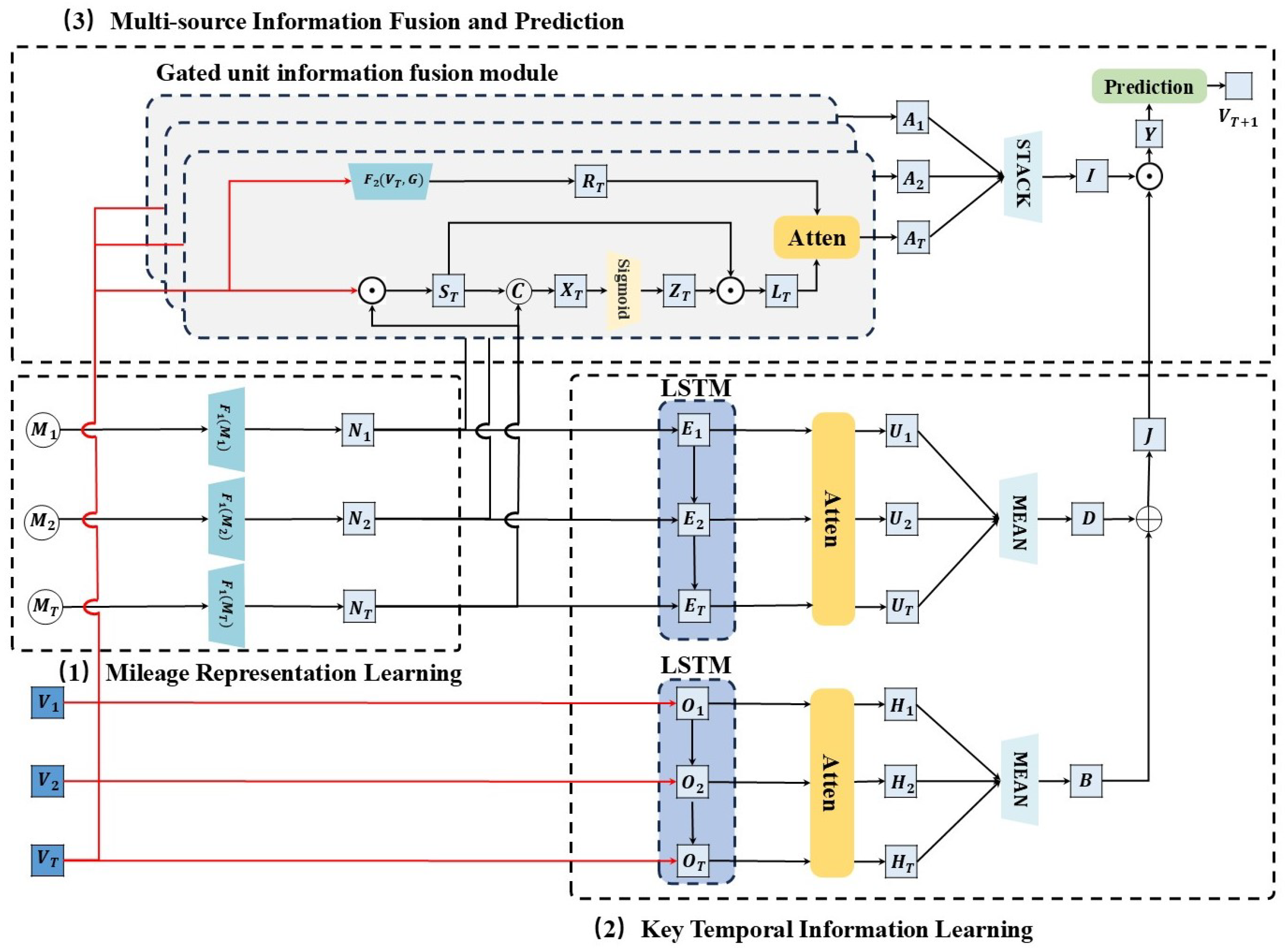
The framework of the proposed Mileage-aware (Mila) model for vehicle maintenance demand prediction is presented in Figure 1. The framework consists of three key modules:
(1) Mileage Representation Learning: We propose a mileage representation approach oriented towards maintenance demand prediction, which aligns mileage in the same vector space as maintenance projects.
(2) Key Temporal Information Learning: A key temporal information extraction module is proposed, combining a long short-term memory (LSTM) network with an attention mechanism to extract key temporal information from historical maintenance projects and mileages.
(3) Multi-source Information Fusion and Prediction: We propose a module for integrating mileage and maintenance projects based on a gated unit to enhance the deep integration. The key temporal information learning outcomes and integrated results are combined to obtain the mileage-aware modeling results, which predict the upcoming maintenance demands.

Table 1.
Notations and descriptions.
Table 1.
Notations and descriptions.
| Notation | Description |
|---|---|
| Set of all maintenance project codes | |
| The maintenance projects for a vehicle | |
| The maintenance projects for t-th maintenance | |
| The maintenance mileages for a vehicle | |
| The representation learning function of | |
| Co-occurrence matrix for all maintenance projects | |
| The correlation-aware learning function of | |
| The correlation-aware learning result of and | |
| The representation learning result of | |
| The hidden state of after LSTM | |
| The hidden state of after LSTM | |
| The key temporal information learning result of | |
| The key temporal information learning result of | |
| B | The comprehensive key temporal information learning result of |
| D | The comprehensive key temporal information learning result of |
| J | The comprehensive key temporal information learning result of and |
| The Hadamard product result of and | |
| The concatenate result of and | |
| The activation result of | |
| The Hadamard product result of and | |
| The fusion result of and | |
| I | The comprehensive fusion result of and |
| Y | The fusion result of I and J |
| Maintenance projects for the ()-th maintenance |
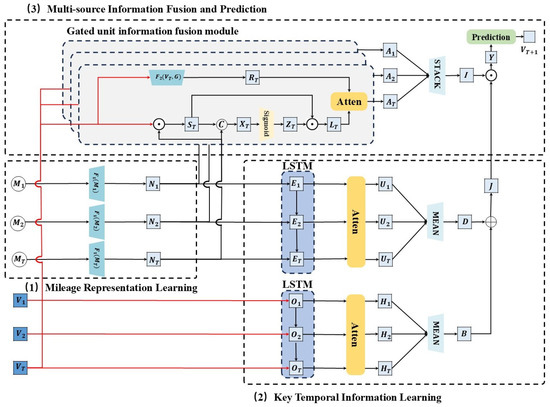
Figure 1.
An overview of the Mila model. It is mainly composed of three modules: (1) mileage representation learning; (2) key temporal information learning; (3) multi-source information fusion and prediction.
Figure 1.
An overview of the Mila model. It is mainly composed of three modules: (1) mileage representation learning; (2) key temporal information learning; (3) multi-source information fusion and prediction.
3.3. Mileage Representation Learning
Mileage is a crucial indicator of vehicle condition. Generally, higher mileage correlates with an increased type and frequency of the required maintenance projects.
In evaluating vehicle maintenance tasks, it is essential for maintenance personnel to first understand the current state of the vehicle, including its historical maintenance projects and mileages. Using this information, maintenance staff can make initial inferences about the ongoing maintenance projects required for the vehicle.
Notably, the raw mileage and the maintenance projects do not reside in the same feature space, necessitating the mapping of to the same feature space as to obtain the transformed result . This mapping is achieved by , as illustrated in Equation(1).
where , , , and are parameters. A common assumption in vehicle maintenance demand prediction is that more recent mileage is more important. Therefore, mileages closer to the most recent one should be emphasized. To achieve this, we use the Sigmoid activation function, which ensures that more recent mileages are more significantly activated.
3.4. Key Temporal Information Learning
In the realm of vehicle maintenance, specific critical projects and mileages significantly affect future maintenance demands. To more effectively capture key temporal information from historical maintenance records, we propose a key temporal information learning method that combines a long short-term memory network (LSTM) [2] with an attention mechanism. Initially, the historical maintenance projects and mileages are processed using the LSTM to derive the hidden states and as delineated in Equation (2).
where the LSTM computation process of Equation (2) is shown in Equation (3), where and denote the weights and biases, denote the hidden state.
Following this procedure, the sequences , and encapsulate the original and cumulative information from successive maintenance records, capturing the long-term dependencies within the historical maintenance sequence. Subsequently, these sequences and are processed with the attention mechanism [21], and the specific implementation process is detailed in Equation (4).
where and . The realization of the above attention mechanism is shown in Equation (5).
where d is the attention dimension and denote the attention weights.
Through this process, the interactions between historical maintenance records are enhanced, and the sequences and acquire essential temporal information that impacts future maintenance demand. The comprehensive essential temporal information learning result J is obtained by summation, as shown in Equation (6).
3.5. Multi-Source Information Fusion and Prediction
During vehicle maintenance, a single session often involves executing multiple distinct projects simultaneously. For instance, activities such as oil change and air filter replacement often occur concurrently, indicating an interdependence among various maintenance projects. To fully utilize the correlations between maintenance projects, we propose a representation based on the co-occurrence matrix.
We create a global co-occurrence graph for all maintenance projects with weighted edges, each node serving as a representation of a maintenance project sourced from the set P. If a pair co-occurs in a vehicle’s maintenance record, two equal weights and are integrated into G. We then count the total co-occurrence frequency of in all vehicle maintenance records for further calculation of edge weights. Additionally, we aim to identify important and common project pairs. Consequently, we define a threshold to filter out combinations with low frequency, resulting in a qualified set for . Let represent the total frequency of qualified projects co-occurring with . We used an adjacency matrix to represent the co-occurrence graph as defined in Equation (7).
Note that G is designed to be symmetric, representing the influence of two maintenance projects. As a static matrix, G quantifies the frequency of global maintenance project co-occurrence. However, the occurrence and disappearance of various maintenance projects happen at different stages. Even if a specific maintenance project is absent from current records, a related project may emerge in the future due to correlations among various projects. Consequently, to account for the correlations among maintenance projects, the correlation representation of each project is derived from each vehicle’s historical maintenance projects , utilizing . The definition of is provided in Equation (8).
By the operation of , contains not only the information of the original maintenance projects, but also implies the information on the previous related maintenance projects.
To better integrate historical maintenance projects and mileage data, we propose an information fusion module based on a gated unit [22] to achieve a more comprehensive integration of projects and mileages on an item-by-item basis. First, we perform a matrix dot product on and to obtain . Then, we subtract from to obtain . Next, is activated by a Sigmoid function to yield . Finally, and are multiplied to produce . The detailed computational procedure is illustrated in Equation (9).
where and denote the weights and biases, respectively. The integration of project and mileage information learned through gated unit enhances the model’s representation. Subsequently, and are fused using the attention mechanism outlined in Equation (5), as demonstrated in Equation (10).
The impact of the project relevance representation on the current gated unit fusion results is dynamically adjusted through an attention mechanism. A weighted representation is generated by calculating the relationships among queries, keys, and values, enabling the model to learn the information embedded in more relevant historical records.
After obtaining the successive projects and mileages fusion results , the combined fusion result is defined as . Element-wise multiplication is employed to enhance the integration of the comprehensive fusion result I and the comprehensive key temporal information learning result J, thereby deriving the fusion result Y, as illustrated in Equation (11).
The maintenance projects of the ()-th maintenance are obtained based on the fusion result Y. The specific realization of the process is shown in Equation (12).
where and are parameters, and is the dimension of Y. To increase the robustness of the model, a dropout operation is performed before Y makes the prediction.
3.6. Model Optimization
We train the Mila model to predict the ()-th maintenance project for each vehicle, with a binary cross-entropy loss function for the global objective function, as shown in Equation (13):
where represents the predicted results of the maintenance project and represents the true label of the maintenance project .
4. Experiment Result and Analysis
4.1. Dataset Description
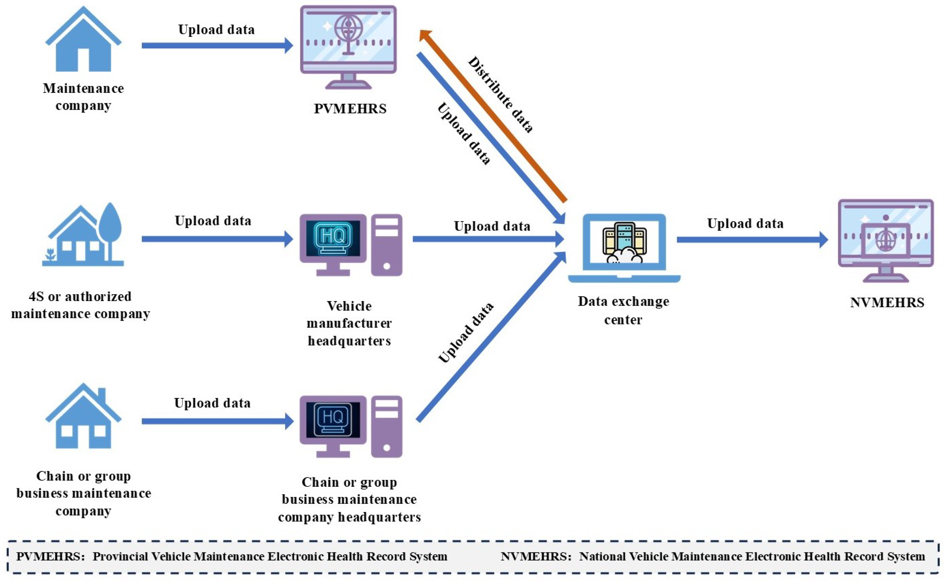
According to the “Provisions on the Administration of Motor Vehicle Maintenance” [23] issued by the Ministry of Transport of China, all vehicle maintenance companies must upload complete maintenance record data of vehicles to the Vehicle Maintenance Electronic Health Record System, as illustrated in Figure 2. Maintenance companies, 4S or authorized maintenance companies and chain or group business maintenance companies individually upload their vehicles’ maintenance record data to the Provincial Vehicle Maintenance Electronic Health Record System, vehicle manufacturer headquarters, and chain or group business maintenance companies’ headquarters. Subsequently, the Provincial Vehicle Maintenance Electronic Health Record System, vehicle manufacturer headquarters, and chain or group business maintenance company headquarters upload the data to the data exchange center. The data exchange center distributes data from each province’s 4S or authorized maintenance companies and chain or group business maintenance companies to the respective provincial systems, concurrently uploading the data to the National Vehicle Maintenance Electronic Health Record System.

Figure 2.
Vehicle maintenance record data collection process.
To evaluate the effectiveness of our proposed method, we randomly selected all maintenance record data of some passenger vehicles from a specific brand from the National Vehicle Maintenance Electronic Health Record System, including the unique identification number of each vehicle, all maintenance projects performed, maintenance time, and mileage. During data preprocessing, we excluded vehicles with fewer than two maintenance records and coded all maintenance projects. The detailed preprocessing steps are as follows:
- Data cleaning: Removed duplicate records;
- Data normalization: Categorized the maintenance projects and coded them into a uniform format;
- Data filtering: Excluded vehicles with incorrect maintenance records and those with fewer than two maintenance records.
The resulting dataset comprises maintenance records for 10,252 vehicles serviced between August 2015 and April 2023 by 35 maintenance companies. The detailed statistics of the dataset are provided in Table 2, and the distributions of the vehicle maintenance records are depicted in Figure 3. To optimize the experimental procedure, the dataset was randomly partitioned into training, validation, and test subsets. The training subset comprises 6000 vehicles, the validation subset includes 3252 vehicles, and the test subset consists of 1000 vehicles. In our methodology, the most recent maintenance projects are designated as the label, while all prior maintenance projects and mileage serve as input features.
Table 2.
Experimental dataset statistics.
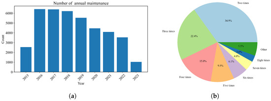
Figure 3.
The distributions of the vehicle maintenance record. (a) The distribution of vehicle maintenance record by the number of annual maintenance projects. (b) The distribution of vehicles by the number of maintenance projects.
4.2. Inputs and Outputs
To train the model, the inputs include all historical maintenance projects and mileages for each vehicle. Specifically, the data include the maintenance projects performed historically and the corresponding mileage when these projects occurred. At runtime, the model requires similar inputs: all historical maintenance projects and their corresponding mileages. This information is used to predict the next maintenance demands of the vehicle.
Regarding the output of the model, the predicted maintenance projects indicate the necessary maintenance operations that should be performed at the next maintenance. These predictions are essential for vehicle maintenance planning to ensure that the necessary interventions are taken in a timely manner to maintain the health and performance of the vehicle. The model outputs are closely related to the dynamics of the vehicle, and the maintenance projects that need to be performed on each system of the vehicle reflect the necessary operations, highlighting potential risks in each area that can affect handling, stability, and vehicle dynamics. Timely maintenance ensures that the systems are functioning properly, thus guaranteeing the dynamics of the vehicle during driving.
In practice, the driver receives information about the necessary maintenance projects for the next maintenance. This information, available through the vehicle’s on-board diagnostic system or maintenance scheduling application, provides clear guidance on necessary maintenance actions, helping to proactively maintain the vehicle and prevent potential problems.
4.3. Baseline Models and Evaluation Metrics
The principal objective of this experiment is to predict the ()-th maintenance projects by leveraging the preceding T maintenance projects and mileages of the vehicle, thereby presenting a multi-label classification challenge. To this end, the evaluation metrics utilized are the weighted F1 score (w-F1) [24] and R@k [24]. The w-F1 score calculates the F1 score for each project code and provides its weighted average, while R@k measures the average ratio of desired project codes among the top k predictions relative to the total desired project codes in each maintenance operation. This metric quantifies prediction accuracy.
To validate the effectiveness of our proposed method, we conducted comparative analyses against several well-established machine learning and deep learning time series prediction techniques, including MLP [25], CNN [26], RNN [27], LSTM [2], and GRU [28]. In addition, we compared our approach with typical existing methods for predicting vehicle maintenance demand, such as SLFN [15], DBN [20], and EFMSAE-LSTM [18]. Furthermore, we evaluated our method against leading approaches in the field of medical diagnosis prediction, which share similarities with maintenance demand prediction, specifically RETAIN [29], Dipole [30], and Chet [24].
4.4. Implementation Details
The principal objective of the experiment was to predict the ()-th maintenance projects using the previous T records. The model parameters were initialized randomly, and hyperparameters, along with activation functions, were calibrated based on the verification set as before. The batch size was maintained at 32 for consistency. During training, the model underwent 100 epochs using Adam optimization algorithms, with the learning rate set at 0.001. The computational tasks were performed using Python 3.12.3 and PyTorch version 2.3.1+cu121. The hardware devices was equipped with 64 GB of memory and NVIDIA GeForce RTX 3090 GPUs (Nvidia, Santa Clara, CA, USA). To maintain robustness and replicability, the experiment was repeated five times, each with a different random seed.
The NVIDIA GeForce RTX 3090 GPU used for the experiments is for model training purposes. In the actual deployment and application of the model, the on-board ECU typically does not possess such high-performance computing resources. Instead, the model inference can be accomplished using lighter embedded computing resources, such as the Cortex-M4/M7 architecture. Techniques such as model quantization, pruning, and edge cloud computing deployment strategies will be explored to ensure the feasibility and efficiency of the model in real vehicle applications. Model quantization reduces the model size and computational load by decreasing the precision of the weights. Pruning involves removing redundant parameters, which helps in reducing the model complexity. Edge cloud computing can offload some computational tasks to nearby cloud servers, balancing the load between the vehicle’s ECU and the cloud.
4.5. Prediction Performance
As demonstrated by the experimental results presented in Table 3, the Mila model significantly outperforms comparative models in maintenance project prediction. Given that the average number of maintenance projects per instance is 5.21, this study defines multiple values of k = ([5,10,15,20,25,30,35]) to thoroughly assess the performance of R@k. The results indicate that the Mila model surpasses all referenced baseline models across both shorter and longer prediction lists. Regarding the w-F1 metric, the Mila model registers a leading score of 40.99 ± 0.21%, surpassing the highest-performing Chet model by 3.56%. Generally, a higher w-F1 score indicates a better balance between precision and recall achieved by the model. Consequently, the Mila model effectively predicts a higher number of accurate maintenance projects while minimizing incorrect predictions, which is critical in practical scenarios. Moreover, the Mila model demonstrates significant advantages across multiple R@k metrics. In summary, the Mila model not only demonstrates high accuracy and generalization capabilities in predicting maintenance projects but also reinforces its utility through consistent performance across various prediction list lengths, establishing a solid foundation for future research and practical applications.
Table 3.
Maintenance project prediction results using w-F1(%) and R@k (%) (the best is in red).
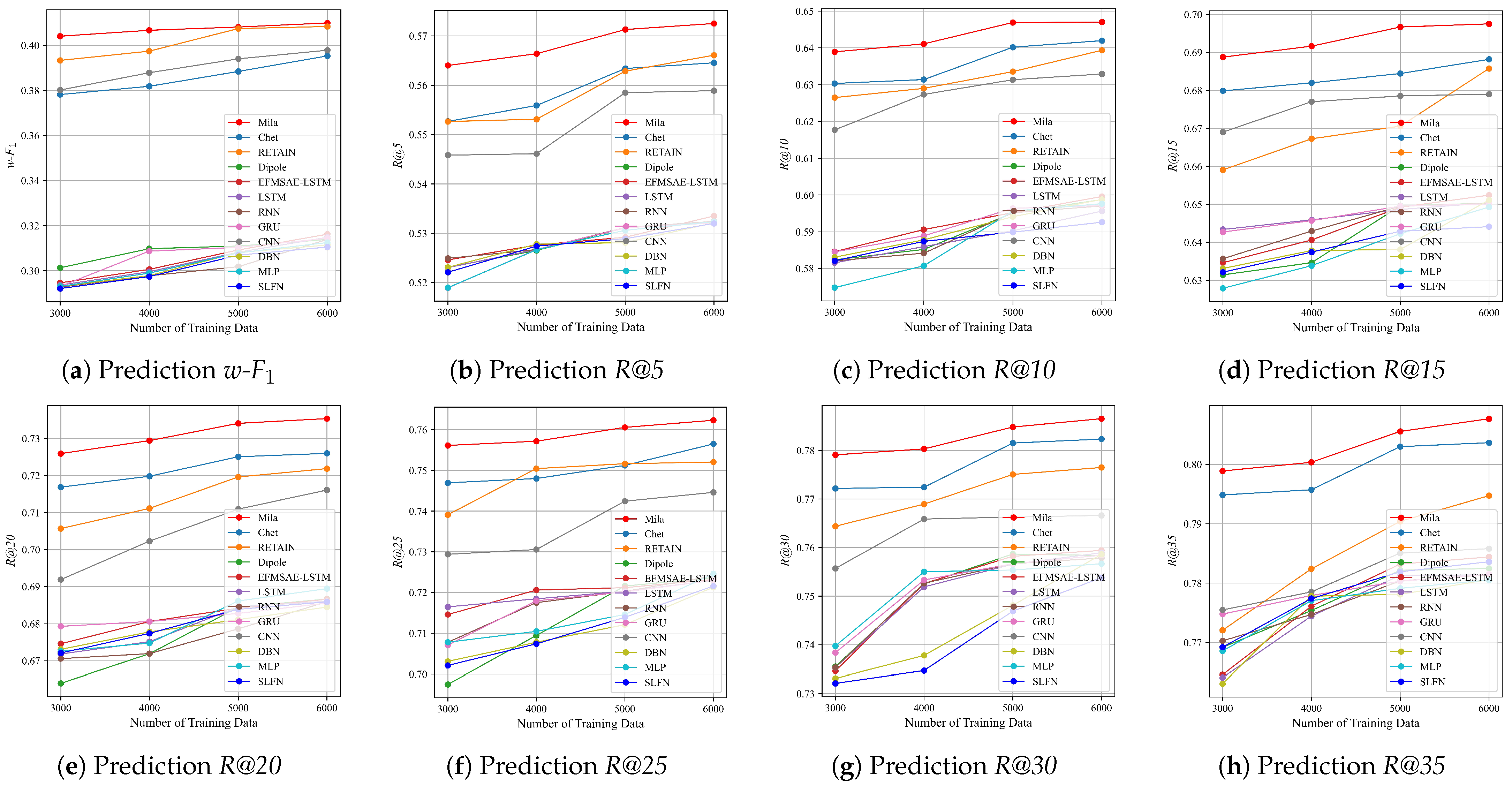
4.6. Performance Evaluation on Data Sufficiency
To assess the impact of data sufficiency on predictive accuracy, we maintain the size of the validation set constant at 3252 entries. We varied the size of the training sets to 3000; 4000; 5000; and 6000, respectively, and utilized the remaining data for the test set. The superior performance of Mila relative to other baseline models, even with limited data, is demonstrated in Figure 4.
4.7. Ablation Study
In order to conduct a thorough analysis of each module’s effectiveness in our proposed model, we compared three ablation variants of the model, each with distinct settings. These variants are as follows:
- Mila-mileage: This variant attempts to elucidate the role of mileage in the model by omitting the input of mileage from the model such that , J = D.
- Mila-atten: This variant attempts to elucidate the role of the attention mechanism by omitting inputs to the attention mechanism from the learning module of key temporal information such that , .
- Mila-gated: This variant accounts for its role in the model by omitting the gated unit information fusion module, making .
The outcomes of the ablation studies, presented in Table 4, reveal several critical conclusions. Initially, each model variant shows a reduced performance compared to the complete Mila model, indicating that mileage, key temporal information learning, and gated unit information fusion are all critical components. The Mila model outperforms the other three variants across all evaluation metrics, notably in w-F1 scores and R@k performance, signifying that each component is crucial for enhancing overall performance.
Table 4.
Ablation study of vehicle maintenance project prediction results using w-F1(%) and R@k (%) (the best is in red).
Several key conclusions can be drawn from the results:
- Overall performance: The complete Mila model demonstrates the highest performance across all evaluation metrics. This indicates that each component (mileage input, key temporal information learning, and gated unit information fusion) is crucial for improving overall performance.
- Component importance: The results for Mila-atten and Mila-gated are comparable; however, Mila-gated marginally outperforms the former in most metrics, suggesting that the attention mechanism might be slightly more crucial than the gated unit information fusion module. Moreover, the performance of Mila-mileage lags behind the other two ablation variants, indicating that mileage plays a significant role in forecasting vehicle maintenance demand.
These findings demonstrate that each module in our proposed model contributes indispensably to the overall performance enhancement.
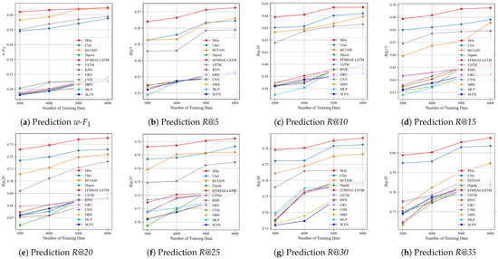
Figure 4.
Accuracy of predictions of Mila and baseline with varying training data.
Figure 4.
Accuracy of predictions of Mila and baseline with varying training data.
4.8. New Maintenance Projects Prediction
In this study, new maintenance projects are defined as those not present in the vehicle’s previous maintenance history. Such predictions are crucial for identifying potential vehicle issues and improving service coverage. Considering the dependency among maintenance projects over mileage, our proposed model is anticipated to exhibit a superior performance in predicting new maintenance projects.
Experimental results for each model’s predictive accuracy in the new maintenance projects are detailed in Table 5. Mila significantly outperforms all baseline models in w-F1 scores, with Chet, the nearest competitor, lagging by approximately three percentage points. Furthermore, Mila demonstrates proficiency in the R@k metric, the proportion of new maintenance projects accurately predicted within the first k predictions, especially at higher k values. For instance, at R@35, Mila surpasses its nearest rival, Chet, by approximately 0.45 percentage points, further underscoring Mila’s efficacy and superiority in predicting new maintenance projects.
From the results, several key conclusions can be drawn:
- Predictive accuracy: The Mila model significantly outperforms all baseline models across all evaluation metrics, demonstrating superior accuracy in predicting new maintenance projects.
- Performance at higher k values: The Mila model exhibits an exceptional performance at higher k values, indicating its ability to more accurately predict new maintenance projects. This is crucial for improving service coverage and identifying potential vehicle issues.
These results demonstrate that the Mila model significantly enhances the predictive accuracy of new maintenance projects by leveraging the dependencies between maintenance projects and mileage within maintenance records. Compared to traditional machine learning methods and basic deep learning frameworks, the Mila model adeptly identifies subtle patterns in maintenance projects and mileage, effectively using this information to predict new maintenance projects.
Table 5.
New maintenance project prediction results using w-F1(%) and R@k (%) (the best is in red).
Table 5.
New maintenance project prediction results using w-F1(%) and R@k (%) (the best is in red).
| Model | w-F1 | R@5 | R@10 | R@15 | R@20 | R@25 | R@30 | R@35 |
|---|---|---|---|---|---|---|---|---|
| SLFN | 13.08 ± 0.16 | 22.12 ± 0.13 | 33.63 ± 0.12 | 36.31 ± 0.13 | 46.25 ± 0.11 | 52.11 ± 0.12 | 53.75 ± 0.22 | 55.53 ± 0.32 |
| MLP | 13.06 ± 0.29 | 22.03 ± 0.19 | 33.29 ± 0.42 | 36.96 ± 0.11 | 46.19 ± 0.36 | 52.13 ± 0.23 | 53.46 ± 0.19 | 55.96 ± 0.24 |
| DBN | 13.04 ± 0.21 | 22.21 ± 0.23 | 33.68 ± 0.12 | 36.61 ± 0.22 | 46.49 ± 0.25 | 52.23 ± 0.27 | 53.86 ± 0.21 | 55.66 ± 0.13 |
| CNN | 17.98 ± 0.54 | 23.96 ± 0.46 | 33.76 ± 0.55 | 40.68 ± 0.50 | 46.23 ± 0.29 | 51.09 ± 0.27 | 55.70 ± 0.33 | 58.99 ± 0.10 |
| GRU | 15.52 ± 0.41 | 21.88 ± 0.45 | 31.68 ± 0.19 | 36.81 ± 0.56 | 43.20 ± 0.64 | 50.28 ± 0.31 | 56.29 ± 0.66 | 58.78 ± 0.48 |
| RNN | 16.85 ± 0.28 | 21.92 ± 0.07 | 29.97 ± 0.16 | 36.86 ± 0.19 | 44.34 ± 0.24 | 51.40 ± 0.39 | 54.02 ± 0.31 | 58.79 ± 0.17 |
| LSTM | 13.35 ± 0.17 | 23.94 ± 0.18 | 30.96 ± 0.20 | 38.27 ± 0.14 | 45.15 ± 0.20 | 49.99 ± 0.13 | 53.82 ± 0.32 | 56.04 ± 0.34 |
| EFMSAE-LSTM | 13.74 ± 0.21 | 23.13 ± 0.12 | 30.68 ± 0.12 | 38.24 ± 0.26 | 45.65 ± 0.23 | 49.36 ± 0.14 | 53.54 ± 0.13 | 56.62 ± 0.22 |
| Dipole | 14.89 ± 0.31 | 23.43 ± 0.00 | 32.94 ± 0.28 | 37.35 ± 0.18 | 45.83 ± 0.17 | 49.21 ± 0.48 | 53.80 ± 0.41 | 59.71 ± 0.31 |
| RETAIN | 18.91 ± 0.50 | 25.02 ± 0.57 | 34.97 ± 0.24 | 41.81 ± 0.37 | 46.10 ± 0.50 | 53.75 ± 0.39 | 56.00 ± 0.42 | 59.73 ± 0.63 |
| Chet | 19.24 ± 0.33 | 26.06 ± 0.33 | 34.24 ± 0.26 | 42.11 ± 0.21 | 46.69 ± 0.21 | 55.23 ± 0.34 | 55.54 ± 0.41 | 62.96 ± 0.56 |
| Mila | 21.97 ± 0.04 | 27.36 ± 0.11 | 37.31 ± 0.06 | 42.97 ± 0.09 | 49.13 ± 0.15 | 56.05 ± 0.22 | 59.52 ± 0.15 | 63.41 ± 0.20 |
4.9. Parameter Sensitivity Analysis
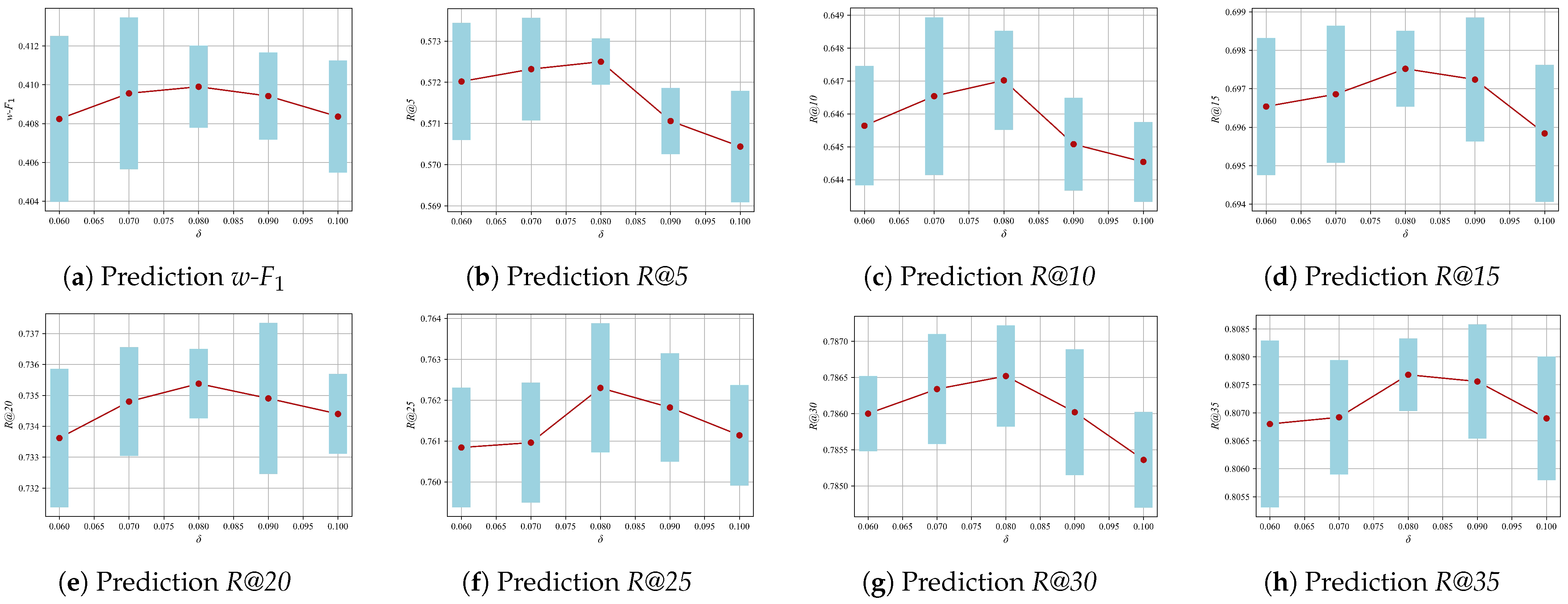
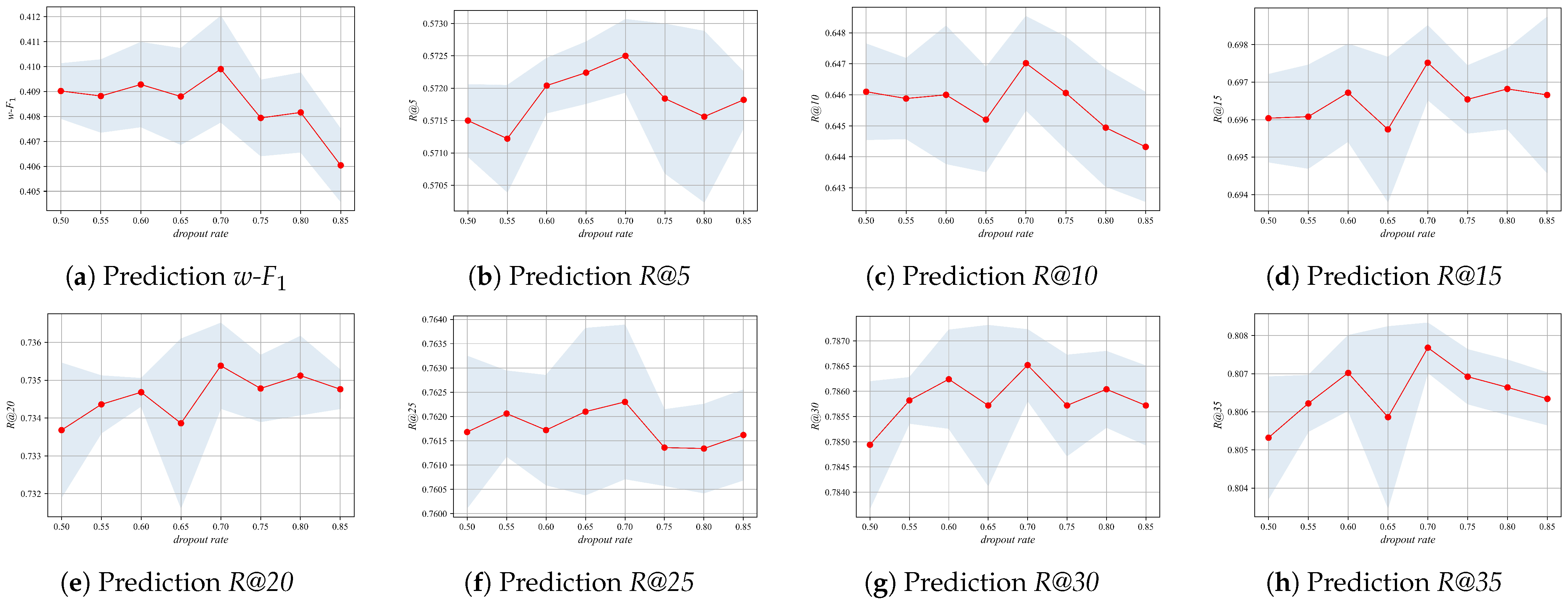
To investigate the influence of Mila’s key hyperparameters on its performance, we examined the impact of the co-occurrence matrix threshold, denoted as , and the dropout rate in Equation (12) on the experimental results. This was achieved by considering thresholds of 0.06, 0.07, 0.08, 0.09, 0.10. As illustrated in Figure 5, the optimal performance is observed at a threshold of 0.08. The dropout rate was set within the range of 0.50–0.85, and the results, as shown in Figure 6, indicate that the optimal performance is achieved at a dropout rate of 0.70.
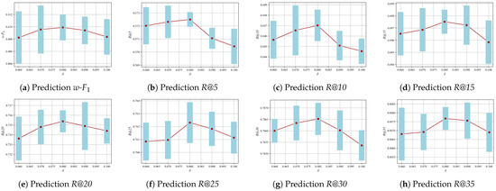
Figure 5.
Parameter sensitivity analysis of .
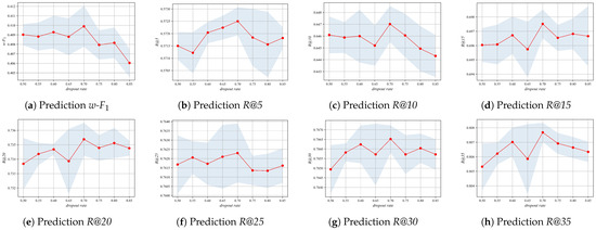
Figure 6.
Parameter sensitivity analysis of dropout rate.
5. Conclusions
To address the limitations of existing methods, which are restricted to partial predictions of vehicle maintenance demand, this paper introduces a mileage-aware model designed to predict the full scope of vehicle maintenance demands. To tackle the issue of significant mileage disparities, we propose a mileage representation method for the maintenance demand prediction task. To capture the substantial impact of key mileage and maintenance projects on future demand, we propose a learning module for key temporal information using a combination of LSTM and attention mechanism. Furthermore, to integrate maintenance projects and mileages, we propose a fusion module using a gated unit. Experimental validation using actual vehicle maintenance records demonstrates that the proposed model outperforms existing techniques, thereby affirming its effectiveness and utility in predicting vehicle maintenance demand.
Although our model shows a superior performance in predicting maintenance demands, it is important to consider that, in real-world applications, these predictions may be clustered by return trip mileage, potentially limiting their practical implementation. in addition, the model is limited to historical vehicle maintenance records, which provide relatively limited information. In future studies, we intend to develop a dynamic adjustment mechanism that accounts for the clustering of predictions by return trip mileage and incorporate explicit vehicle maintenance technology information into the prediction task. This will improve the adaptability and interpretability of our model and further advance the field.
Author Contributions
F.C. contributed to the data analysis, algorithm construction, and writing and editing of the manuscript. D.S., G.Z. and F.R. reviewed and edited the manuscript. K.Y. proposed the idea and contributed to the data acquisition, performed supervision, and project administration, and reviewed and edited the manuscript. All authors have read and agreed to the published version of the manuscript.
Funding
This research received no external funding.
Data Availability Statement
The data presented in this study are available upon request from the corresponding author due to privacy.
Conflicts of Interest
The authors declare no conflicts of interest.
References
- Chen, C.; Liu, Y.; Sun, X.; Di Cairano-Gilfedder, C.; Titmus, S. Vehicle maintenance prediction using deep learning with GIS data. In Procedia CIRP; Elsevier: Amsterdam, The Netherlands, 2019; Volume 81, pp. 447–452. [Google Scholar]
- Hu, H.; Luo, H.; Deng, X. Health monitoring of automotive suspensions: A lstm network approach. Shock Vib. 2021, 2021, 6626024. [Google Scholar] [CrossRef]
- Begni, A.; Dini, P.; Saponara, S. Design and test of an lstm-based algorithm for li-ion batteries remaining useful life estimation. In Proceedings of the International Conference on Applications in Electronics Pervading Industry, Environment and Society, Genoa, Italy, 26–27 September 2022; Springer: Berlin/Heidelberg, Germany, 2022; pp. 373–379. [Google Scholar]
- Dini, P.; Basso, G.; Saponara, S.; Romano, C. Real-time monitoring and ageing detection algorithm design with application on SiC-based automotive power drive system. IET Power Electron. 2024, 17, 690–710. [Google Scholar] [CrossRef]
- Zhao, Y.; Liu, P.; Wang, Z.; Hong, J. Electric vehicle battery fault diagnosis based on statistical method. Energy Procedia 2017, 105, 2366–2371. [Google Scholar] [CrossRef]
- Wang, M.-H.; Chao, K.-H.; Sung, W.-T.; Huang, G.-J. Using ENN-1 for fault recognition of automotive engine. In Expert Systems with Applications; Elsevier: Amsterdam, The Netherlands, 2010; Volume 37, pp. 2943–2947. [Google Scholar]
- Jeong, K.; Choi, S. Model-based Sensor Fault Diagnosis of Vehicle Suspensions with a Support Vector Machine. Int. J. Automot. Technol. 2019, 20, 961–970. [Google Scholar] [CrossRef]
- Vasavi, S.; Aswarth, K.; Pavan, T.S.D.; Gokhale, A.A. Predictive analytics as a service for vehicle health monitoring using edge computing and AK-NN algorithm. Mater. Today Proc. 2021, 46, 8645–8654. [Google Scholar]
- Ma, M.; Wang, Y.; Duan, Q.; Wu, T.; Wang, Q. Fault detection of the connection of lithium-ion power batteries in series for electric vehicles based on statistical analysis. Energy 2018, 164, 745–756. [Google Scholar] [CrossRef]
- Zhou, Y.; Zhu, L.; Yi, J.; Luan, T.H.; Li, C. On Vehicle Fault Diagnosis: A Low Complexity Onboard Method. In Proceedings of the GLOBECOM 2020—2020 IEEE Global Communications Conference, Taipei, Taiwan, 7–11 December 2020; IEEE: Piscataway, NJ, USA, 2020. [Google Scholar]
- Shen, D.; Wu, L.; Kang, G.; Guan, Y.; Peng, Z. A novel online method for predicting the remaining useful life of lithium-ion batteries considering random variable discharge current. Energy 2021, 218, 119490. [Google Scholar] [CrossRef]
- Aye, S.A.; Heyns, P.S. An integrated Gaussian process regression for prediction of remaining useful life of slow speed bearings based on acoustic emission. Mech. Syst. Signal Process. 2017, 84 Pt A, 485–498. [Google Scholar] [CrossRef]
- Revanur, V.; Ayibiowu, A.; Rahat, M.; Khoshkangini, R. Embeddings based parallel stacked autoencoder approach for dimensionality reduction and predictive maintenance of vehicles. In IoT Streams for Data-Driven Predictive Maintenance and IoT, Edge, and Mobile for Embedded Machine Learning: Second International Workshop, IoT Streams 2020, and First International Workshop, ITEM 2020, Co-Located with ECML/PKDD 2020, Ghent, Belgium, September 14–18, 2020, Revised Selected Papers 2; Springer: Berlin/Heidelberg, Germany, 2020; pp. 127–141. [Google Scholar]
- Khoshkangini, R.; Sheikholharam Mashhadi, P.; Berck, P.; Gholami Shahbandi, S.; Pashami, S.; Nowaczyk, S.; Niklasson, T. Early prediction of quality issues in automotive modern industry. Information 2020, 11, 354. [Google Scholar] [CrossRef]
- Tessaro, I.; Mariani, V.C.; Coelho, L.S. Machine learning models applied to predictive maintenance in automotive engine components. Proceedings 2020, 64, 26. [Google Scholar] [CrossRef]
- Biddle, L.; Fallah, S. A novel fault detection, identification and prediction approach for autonomous vehicle controllers using SVM. In Automotive Innovation; Springer: Berlin/Heidelberg, Germany, 2021; Volume 4, pp. 301–314. [Google Scholar]
- Al-Zeyadi, M.; Andreu-Perez, J.; Hagras, H.; Royce, C.; Smith, D.; Rzonsowski, P.; Malik, A. Deep learning towards intelligent vehicle fault diagnosis. In Proceedings of the 2020 International Joint Conference on Neural Networks (IJCNN), Glasgow, UK, 19–24 July 2020; IEEE: Piscataway, NJ, USA, 2020; pp. 1–7. [Google Scholar]
- Guo, J.; Lao, Z.; Hou, M.; Li, C.; Zhang, S. Mechanical fault time series prediction by using EFMSAE-LSTM neural network. Measurement 2021, 173, 108566. [Google Scholar] [CrossRef]
- Safavi, S.; Safavi, M.A.; Hamid, H.; Fallah, S. Multi-sensor fault detection, identification, isolation and health forecasting for autonomous vehicles. Sensors 2021, 21, 2547. [Google Scholar] [CrossRef] [PubMed]
- Xu, P.; Wei, G.; Song, K.; Chen, Y. High-accuracy health prediction of sensor systems using improved relevant vector-machine ensemble regression. Knowl.-Based Syst. 2021, 212, 106555. [Google Scholar]
- Vaswani, A.; Shazeer, N.; Parmar, N.; Uszkoreit, J.; Jones, L.; Gomez, A.N.; Kaiser, L.; Polosukhin, I. Attention is all you need. In Proceedings of the Advances in Neural Information Processing Systems 30 (NIPS 2017), Long Beach, CA, USA, 4–9 December 2017; pp. 6000–6010. [Google Scholar]
- Dauphin, Y.N.; Fan, A.; Auli, M.; Grangier, D. Language modeling with gated convolutional networks. In Proceedings of the 34th International Conference on Machine Learning, Sydney, Australia, 6–11 August 2017; pp. 933–941. [Google Scholar]
- Ministry of Transport of the People’s Republic of China. Decision on Amending the Provisions on the Administration of Motor Vehicle Maintenance. Order No. 14 [2023], 10 November 2023. Available online: https://www.gov.cn/gongbao/2024/issue_11146/202402/content_6930538.html (accessed on 20 February 2024).
- Lu, C.; Han, T.; Ning, Y. Context-aware Health Event Prediction via Transition Functions on Dynamic Disease Graphs. In Proceedings of the AAAI Conference on Artificial Intelligence, Online, 22 February–1 March 2022; pp. 2982–2989. [Google Scholar]
- Rumelhart, D.E.; Hinton, G.E.; Williams, R.J. Learning representations by back-propagating errors. Nature 1986, 323, 533–536. [Google Scholar] [CrossRef]
- Krizhevsky, A.; Sutskever, I.; Hinton, G.E. ImageNet classification with deep convolutional neural networks. In Proceedings of the Advances in Neural Information Processing Systems 25 (NIPS 2012), Lake Tahoe, NV, USA, 3–6 December 2012; pp. 1097–1105. [Google Scholar]
- Elman, J.L. Finding structure in time. Cogn. Sci. 1990, 14, 179–211. [Google Scholar] [CrossRef]
- Cho, K.; Van Merriënboer, B.; Gulcehre, C.; Bahdanau, D.; Bougares, F.; Schwenk, H.; Bengio, Y. Learning phrase representations using RNN encoder-decoder for statistical machine translation. arXiv 2014, arXiv:1406.1078. [Google Scholar]
- Choi, E.; Bahadori, M.T.; Kulas, J.A.; Schuetz, A.; Stewart, W.F.; Sun, J. RETAIN: An interpretable predictive model for healthcare using reverse time attention mechanism. In Proceedings of the 30th International Conference on Neural Information Processing Systems, Barcelona, Spain, 5–10 December 2016; pp. 3504–3512. [Google Scholar]
- Ma, F.; Chitta, R.; Zhou, J.; You, Q.; Sun, T.; Gao, J. Dipole: Diagnosis prediction in healthcare via attention-based bidirectional recurrent neural networks. In Proceedings of the 23rd ACM SIGKDD International Conference on Knowledge Discovery and Data Mining, Halifax, NS, Canada, 13–17August 2017; pp. 1903–1911. [Google Scholar]

Disclaimer/Publisher’s Note: The statements, opinions and data contained in all publications are solely those of the individual author(s) and contributor(s) and not of MDPI and/or the editor(s). MDPI and/or the editor(s) disclaim responsibility for any injury to people or property resulting from any ideas, methods, instructions or products referred to in the content. |
© 2024 by the authors. Licensee MDPI, Basel, Switzerland. This article is an open access article distributed under the terms and conditions of the Creative Commons Attribution (CC BY) license (https://creativecommons.org/licenses/by/4.0/).