Abstract
Despite the increase in the efficiency of energy consumption in information and communication technology, software execution and its constraints are responsible for how energy is consumed in hardware hosts. Consequently, researchers have promoted the development of sustainable software with new development methods and tools to lessen its hardware demands. However, the approaches developed so far lack cohesiveness along the stages of the software development life cycle (SDLC) and exist outside of a holistic method for green software development (GSD). In addition, there is a severe lack of approaches that target the analysis and design stages of the SDLC, leaving software architects and designers unsupported. In this article, we introduce our behavior-based consumption profile (BBCP) external Domain-Specific Language (DSL), aimed at assisting software architects and designers in modeling the behavior of software. The models generated with our external DSL contain multiple sets of properties that characterize features of the software’s behavior. In contrast to other modeling languages, our BBCP emphasizes how time and probability are involved in software execution and its evolution over time, helping its users to gather an expectation of software usage and hardware consumption from the initial stages of software development. To illustrate the feasibility and benefits of our proposal, we conclude with an analysis of the model of a software service created using the BBCP, which is simulated using Insight Maker to obtain an estimation of hardware consumption and later translated to energy consumption.
1. Introduction
The assessment of global economies in terms of gross economic growth has been previously criticized as an unsustainable metric [1], as its reliance on the limited availability of natural resources to manufacture, distribute, and maintain the goods and services we consume has environmental consequences we incrementally see signs of. The consensus is that a global reduction of both the amount and rhythm of natural resource consumption is the best strategy against the environmental strain we impose. Contrary to the previous notion, as millions of ICT (Information and Communication Technology) devices are deployed into our global network with each passing year, ICT researchers are concerned with reducing the energy consumption of software as a strategy for degrowth—the ability to perform computation with scarce of resources or energy [2].
The efforts that address degrowth have resulted in a relatively new branch of studies called green software development (GSD), also known, or misunderstood, as sustainable software [3]. The democratization of green software methods and tools is a big issue, as software engineers and developers are increasingly aware of the relevance of the energy consumption of software [3,4,5], which includes the expense of its execution and construction. Still, they are powerless when trying to improve it themselves, as they are riddled by technicalities [6].
We agree with the authors of previous studies that supporting software architects and designers from the initial stages of the SDLC with a green software design methodology will help them to create increasingly frugal software [3,7,8], promoting, in turn, the democratization of GSD. The objectives we have identified to prove our hypothesis are the following: (1) the creation of a platform-agnostic software behavior modeling approach that includes uncertainty as a factor in software design, (2) the creation of energy consumption ratings per type of software using the software models, and (3) the assessment and suggestion of changes in the behavior of the software models to improve the efficiency of the final software.
In this article, we present our full-fledged proposal, called behavior-based consumption profiles (BBCPs), which significantly extends and improves our previous preliminary seminal paper [9]. The BBCP is an external DSL developed as a response to the severe lack of support that green software development (SDLC) has received for the analysis and design stages of the software development life cycle (SDLC), and the aforementioned first objective. The novelty and main contribution of our proposal lie in our method of modeling software behavior-based on time-based, stochastic, and changing descriptions of architectural, business, and user constraints, which represents a significant step towards a holistic description of software behavior focused on energy estimations. Some of the key contributions include the following:
- The probabilistic nature of our software-behavior modeling approach enables software designers to effectively manage the uncertainty of human–computer interactions (HCIs), thereby anticipating prospective energy consumption before any code is written and test-users are involved.
- We introduce the concept of diachronic software design, emphasizing the importance of software design that is conscious of time restrictions and changes in user demand over time.
- The BBCP simplifies the modeling of resource-intensive scenarios, which typically require extensive data collection and user testing.
As opposed to existing works, our approach emphasizes the importance of time constraints and the evolution of the user demand in time, and, therefore, it can represent expected usage scenarios more closely. In addition, the insights gained by using our approach can be used later on in the development process, as illustrated in Figure 1.
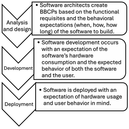
Figure 1.
Target benefits of the BBCP along the SDLC.
The rest of this article is structured as follows. In Section 2, we delve into the existing research concerning software behavior description, setting the stage for the introduction of each component of our behavior-based consumption profiles approach in Section 3. Following this, in Section 4, we offer an illustrative example of a couple of software models crafted using our approach. This example serves to showcase and briefly discuss the results generated through our system model. Finally, we draw our article to a close with a summary of our findings and directions for future research in Section 6.
2. Related Work
A central point to our research is the differentiation between the behavior of software and the behavior with software, key to understanding the criteria for comparison of our approach against pre-existing DSLs and software modeling approaches. We have found that the term “software behavior” is frequently and loosely used, and it is broadly defined in sources such as the SWEBOK [10] and the Dictionary of Computer Science [11]. In consequence, we created a hybrid definition using a pair of loose pre-existing definitions [12,13] and our considerations, which will be used throughout the article.
To us, the behavior of software is “the collection of functions/methods, variables involved in the functions/methods, and the involvement of external entities required to produce a predictable outcome, all limited to a single unit of software”. As we have previously mentioned, our research also involves “behavior with software”. We define the behavior with software as “the interactions of a software agent or non-digital agent with its environment, ignoring the inner workings of the agent itself”, where a software agent is an autonomous software entity that can summon itself proactively or reactively, and operate in its environment without a user’s intervention. Finally, non-digital agents conserve the attributes of a software agent but they can be partially controlled or influenced by software and can act upon a tangible environment. Some examples of non-digital agents include human users and autonomous machines in cyber-physical systems. We designate human users as non-digital agents because, although they do not host software themselves, they can form relationships with software and software agents. These relationships have the potential to impact the physical world. In the analysis phase of the SDLC, the behavior with software is useful to comprehend how the human–computer interaction (HCI) will affect software behavior and vice versa, denoting how energy relationships can be created between the user and the software.
With the previous considerations in mind, we performed a literature review to find pre-existing DSLs and modeling languages that could support the diachronic software design that we propose, to decide if the development of the BBCP, an interpreter, and a tool to support it were worthy. The methodology we followed for the review, briefly put, was the following:
- A search using Harzing’s Publish or Perish software [14] in Google Scholar’s repository with the following query: SOA AND (green software profiling OR sustainability OR green OR software behavior OR profiling).
- As exclusion criteria, we discarded the papers unrelated to computer science, software engineering, or human–computer interaction, with only 39 papers remaining out of the original 500.
- We read the abstracts of the remaining papers and articles, and discarded the ones with no relevance to the topic, concluding with 11 final papers.
- We read the 11 remaining papers and matched them against 11 criteria. The criteria used for the comparison are available in Table 1, and the results of the process are available in Table 2.
 Table 1. Criteria used to compare the existing approaches to useful features.
Table 2. Comparison among the existing approaches and our behavior-based consumption profiles.
Table 1. Criteria used to compare the existing approaches to useful features.
Table 2. Comparison among the existing approaches and our behavior-based consumption profiles.
Our research revealed the following. On the one hand, approaches that deal with the behavior with software include taking into account human personality profiles to generate believable bot behaviors for a game tournament [21], prototyping intelligent systems that adapt their behavior to match a profile of the user [28], and the simulation of real user behavior on the Internet using machine learning techniques [20]. On the other hand, several examples of software behavior include studying the behavior of embedded systems in component-based software development according to different signal flows [19], modeling an application and resource behavior with profiles in heterogeneous environments [22], and the creation of behavioral profiles built in UML (Unified Modeling Language) to specify the architectural behavioral rules of applications [18].
Most of the previous works make use of a common technique: profiling. Profiling allows researchers to study the specific part of a subject by taking its descriptive elements and characterizing a profile with them. For example, in [22], the behavioral profile of an application takes place in the form of UML stereotypes that allow researchers to trace the patterns of interactions among applications. Similar approaches include the one proposed by Ponsard et al. [26], where the authors propose UML profiles to describe related energy requirements and KPI metrics to application design and deployment elements. Similarly to Ponsard et al., The Object Management Group, responsible for overseeing UML, has created an extension adding support for Real-Time and Embedded Systems in UML, called the UML profile for MARTE [29]. For instance, Shorin et al. [27] proposed an extension of UML models that get transformed into a stochastic Petri net for their stochastic energy consumption analysis, including MARTE.
Other approaches aim to model software’s and services’ behavior with their language, specifically behavioral relationships among software units. For instance, in [16], the authors propose a software behavior modeling language that differentiates itself by supporting business analysts and software architects from the initial phases of the SDLC. To our knowledge, most existing approaches do not describe diachronic behavior (how behavior and even its changes, change over time) that includes elements of uncertainty such as Human-Provided Services (HPSs) [30], where people are actors that affect and constrain a system’s behavior [15,31], reaching into the field of HCI [32] to study how the factors surrounding the user affect the consumption of a unit of software. This is a fundamental issue for our research and contribution, as a secondary goal is to be able to provide energy ratings based on these features.
To conclude, we found that (1) most of the existing works employ profiling, (2) some of the approaches target software behavior modeling from the initial stages of the SDLC, and (3) none of the existing approaches factor software’s or user’s behavioral change into the profiles of software behavior they produce. Therefore, to tackle these shortcomings, our proposal employs a holistic profiling approach that allows software designers and architects to include the uncertainty of HCI, the constraints of the business, and the architectural constraints of software in profiles of the software’s behavior. The resulting profiles can be later analyzed by our custom interpreter, which creates a prospective, changing software usage, which is turned into energy consumption, all from the analysis and design stages of the SDLC.
3. Elements of the BBCP
As we previously mentioned, the behavior-based consumption profile is an external DSL specialized in describing timed-based behavioral patterns and their change over time. External DSLs are a sub-category of DSLs that are implemented via an independent interpreter or compiler. The PlantUML DSL, for instance, is an open-source tool that employs its own text-based language and own interpreter to create diagrams. In the case of the BBCP, we chose JSON (JavaScript Object Notation) to create its base schema as it is human-readable, object-oriented, it supports arrays, and it is popularly used. Furthermore, we used JSON arrays and object-oriented notation to organize concepts into categories that hold multiple objects. It is important to emphasize that we do not discard other text formats or markup languages to implement the BBCP schema if they support key–value pairs, objects, and arrays. The BBCP schema could be easily implemented in XML, for example. A website that contains the BBCP JSON schema and a directory to the subsequent information used in this article is also available [33].
We have completed a prototype of the interpreter that translates the JSON schema and the value of each property in it into a behavior. The interpreter, succinctly explained, receives a BBCP profile as the reference for the initial values for each property, which are later used in a simulation loop where the state of the profile is defined through a randomized process defined by the properties in this section. In addition, to generate a simulation, the pre-requirements of the interpreter are (1) the total simulated time to interpret the profiles for, and (2) one or more profiles. Furthermore, we refer to a dynamic representation of a static BBCP within the interpreter as an instance. The dynamic BBCP (an instance) is an interpreter-generated BBCP whose values and behavior change according to the values defined in the static (or original) BBCP fed to the interpreter. For the remainder of this section, we will explain the properties available in the BBCP, their possible values, and their desired outcome for how the interpreter uses them to generate a behavior within a simulation.
In this text, we include multiple resources to better understand the BBCP. The first resource is a glossary (see Table 3), which explains the concept of each category in the BBCP and how they agglomerate to the definition of behavior in the context of this work. An illustration of a workflow that includes the BBCP in an iterative methodology for software development is available in Figure 2. The illustrated workflow is not limited to iterative methodologies, as the BBCP could be a prototype of behavior and not necessarily a fragment of documentation, which fosters its adoption in evolutive development methodologies such as Agile. The inclusion of the BBCP in diverse development methodologies will be further discussed in Section 5. A conceptual class diagram that describes the dependencies, multiplicity, and life cycle of each element of the BBCP is available in Figure 3. The class diagram must be taken into account to build correct BBCPs, as the general behavior is the product of every element respecting its corresponding rules; more information on constructing correct BBCPs can be found in Appendix B. Finally, we include a table with relational graphs in Figure 4, whose contents extend the information of Figure 3 with the properties within each category and how they are nested. Figure 3 can be thought as a component view of the BBCP, while Figure 4 concentrates on a granular view of the properties in each category.
Table 3.
Core concepts of the BBCP approach.
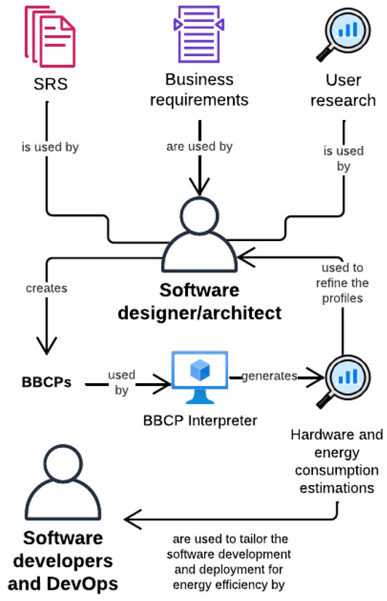
Figure 2.
The involvement of the SDLC actors with the BBCP and its results.
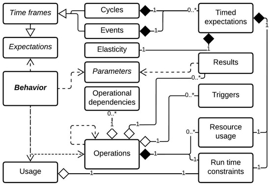
Figure 3.
Conceptual meta-model class diagram explaining the relationships among the core concepts of the BBCP approach.
3.1. Usage Constraints
This category groups the properties responsible for switching between the binary state of an instance, run and stop. The properties are located in row 1 of Figure 4. The run state represents an instance actively consuming resources and exhibiting a behavior, whereas stop represents the opposite. To specify the frequency at which the interpreter samples instances, we utilize the Profile Evaluation Rate property, with Hz as its metric. Conceptually speaking, the value of this property creates periodical points in time when an instance is sampled to learn its state and trigger its changes in behavior and consumption of resources; we call it evaluation.
We created the property Default Run Probability to support the modeling of a higher uncertainty in the behavior of an instance as a representation of unknown external factors, such as the user behavior. This property controls the chance of an instance entering a run state when it is evaluated during a stop state. The Default Stop Probability represents a specific probability for an instance to switch to a stop state when it is evaluated under a run state. When the two preceding properties’ values are set to 0, the only possible way for an instance to enter a run state is if it is triggered by one of its operations due to a dependency relationship with another instance. This will be further discussed in Section 4. If we wanted to describe a coin flip, we could use a Profile Evaluation Rate of 1 Hz, a Default Run Probability of 0.5, and a Default Stop Probability of 0.5. The result is a behavior where a coin toss is performed every second and either state of an instance can be considered heads or tails.

Figure 4.
The BBCP properties and their order.
Figure 4.
The BBCP properties and their order.

3.2. Run Constraints
The objective of the properties in this category is to constrain the time an instance spends active (in a run state). The interpreter measures the time that the instance spends in an active state using two metrics: instant run time and accumulated run time. The instant run time is the duration of the last occurrence of an instance in a run state, in seconds. The accumulated run time is the sum of all the time that an instance spent in a run state in seconds.
The property Minimum Run Time prevents an instance from switching back to a stop state during an evaluation unless the instant run time is greater than this property’s value, in seconds. The property Maximum Run Time, as opposed to Minimum Run Time, limits the instant run time to a maximum duration in seconds. If a run exceeds this limit, the instance is immediately switched to a stop state. The last couple of properties are important to prevent edge cases where an instance can spend either too little or too much time in a run state.
The property Quota is similar to Maximum Run Time but it limits the accumulated run time. The Quota decreases with each second that an instance spends in a run state, hence the name. Once it is depleted, the instance is switched to a stop state and ceases to be evaluated. It will not be evaluated and be able to switch to a run state again unless its Quota is reset. Going forward, we will refer to this specific pattern of behavior as a Depleted Quota.
The Cooldown property defines how long an instance spends with a Depleted Quota before its Quota is replenished and the instance can be re-evaluated. Even though we have constrained the instant run time and the accumulated run time, there could be a need for constraining the instant run time of an instance to a specific duration, which is achieved with Countdown. When the instant run time equals the value of the Countdown, the instance is immediately switched to a stop state.
To summarize how usage constraints and run constraints are utilized, let us think of an example of a surveillance system, more specifically, the software responsible for recording suspicious activity. As per a hypothetical surveillance policy, the software must record at least 10 min of footage with 5 min between recordings. However, if the system sees it fit to do so due to uncontrolled variables, such as a motion sensor, the footage could keep rolling up to 20 min with a maximum daily footage duration of 1200 min (20 h). To replicate this behavior, we can use a Profile Evaluation Rate equal to 0.00333 Hz, as we have to record every 5 min. A Default Run Probability of 1 and a Default Stop Probability of 0.7 can control an irregular switch between states every 5 min. However, to enforce a minimum of 10 min of footage and a maximum of 20, we set the Minimum Run Time to 600 s (10 min) and the Maximum Run Time to 1200 s (20 min). To enforce the maximum daily footage, the Quota is set to 72,000 s (1200 min), and the Cooldown is dynamically set (set by the interpreter) to the time left until the next day. The final result is a behavior that complies with the deliberate requirements of the software in addition to the variability of uncontrolled circumstances that could affect the results. The plot in Figure 5 describes the change in the recording state of the camera according to its usage and run constraints over 3 h.
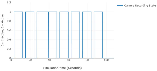
Figure 5.
A plot of the change of the recording state of the camera throughout a simulation.
3.3. Expectations Constraints
Expectations is a category dedicated to bounding the behavior during specific hours and days when changes in the behavior of the software are applied. In adherence to the concepts in Table 3 as well as Figure 3, we placed two sub-categories within expectations: cycles and events, as multiple instances of both can exist per profile. The properties in this category relate to the goals specified in criteria C2, C6, C7, and C10 of Table 1.
3.3.1. Cycles
Cycles contain constraints that repeat during specific days of a week, month, or a deliberate set of days. There are two main properties inside cycles: scale and days. The scale property defines a static amount of days when a cycle could apply. The days property defines a selection of days in a scale when the constraints of the cycle apply. For instance, a scale value of 7 represents a week, and a days value of [6, 7] selects the weekends. Therefore, the same constraints will apply during the weekend for every week, a recurring pattern of behavior. The scale can never be greater than the total duration of the simulation. Following the example of a scale equal to 7, the duration of the simulation to generate with the interpreter would have to be at least equal to 7 days. An example of how cycles are useful can be found in enterprise applications. Let us think of a communication enterprise application running in the company’s server, which is used much more during the week than the weekends. A cycle could be defined for each segment of the week: [1–5] for the weekdays and [6, 7] for the weekends.
3.3.2. Events
In contrast to cycles, events have a single occurrence in time. The Initial Day property defines a day selection in which the time frame for the event is started. Its ending day selects the day after which the constraints of an event will not be effective. If a simulation inside the interpreter were to last 14 days, an event’s Initial Day’s value would be constrained to Initial Day and its End Day’s value to Initial Day ≤ End Day . In the same way that the interpreter validates the length of cycles, the length of events must always be within a valid duration of a simulation in the interpreter. Coming back to the enterprise application example, perhaps the first Monday of the month is when the application is used the most; therefore, it could be isolated by creating an event with the Initial Day set to 1 and the End Day set to 1, overriding the definition of the first cycle for the Day 1 with a scale of 28 days.
To date, we have explained how cycles and events are a part of expectations, which create bounds in time. To complete these bounds, the properties in the timed expectations sub-category constrain the changes in the behavior of an instance during applicable hours.
3.4. Timed Expectations Constraints
This sub-category contains the properties responsible for altering the behavior of an instance during specific bounds of hours, as per C2, and during applicable cycles and events. There are three properties inside timed expectations: Run Probability Override, Stop Probability Override, and Time Range. The value of the Run Probability Override property, as the name implies, overrides the Default Run Probability of the usage category. The Stop Probability Override property does the same but for the Default Stop Probability. The property Time Range creates a selection of hours within a day when the aforementioned properties of this category affect the profile, e.g.: a range of hours for the evening [17–20]. In the same way that timed expectations can override the run and stop probabilities, they can override the values of the run constraints in the usage category when the timed expectation is applicable (see cell 2 of column 2 in Figure 4).
Despite the flexibility that expectations give us to model time-related business constraints, the change in human interactions, and the change in time-related software constraints, we wanted to give architects and designers the possibility to refine the changes during timed expectations even more. This is rooted in the need to profile HPSs, as described in Criteria 10, where the satisfaction of the user can impact on the behavior with software. To solve this we created our next category: elasticity.
3.5. Elasticity Constraints
The properties inside this category go hand-in-hand with timed expectations; therefore, instances of timed expectations have a unique set of elasticity within them, as seen in Figure 3, the same reason why elasticity only works as long as its corresponding timed expectations apply. When the property elasticity is set to true, the values of the properties responsible for probabilities will be modified with slight increases and decreases in value with each evaluation. This constant increase and decrease is where this feature takes its name from.
The first properties that increase the values of the run and stop probabilities are the Positive Run Probability Modifier and the Positive Stop Probability Modifier. The Positive Run Probability Modifier increases, when applicable, either the Default Run Probability or the Run Probability Override with each evaluation for as long as an instance remains in a stop state. The Positive Stop Probability Modifier does the same but for the stop probability as long as the instance remains in a run state.
The properties responsible for the decrease in the values of the run and stop probabilities are the Negative Run Probability Modifier and the Negative Stop Probability Modifier. This pair of properties is similar to the aforementioned ones, but it affects the ongoing state. For example, if an instance is in a run state, the Negative Run Probability Modifier affects the run probability’s value (either the override or the default value) during evaluations, for as long as the instance remains in a run state.
We then added four properties that control a ceiling and the floor for the total run or stop probability, so that edge cases and rebound effects can be taken into account. The two properties that control the ceiling for each value are the Maximum Run Probability and the Maximum Stop Probability. The two properties that control the floor for each value are the Minimum Run Probability and the Minimum Stop Probability. Once a probability has reached either its lowest or highest value, it will stay there unless it is affected in the inverse direction of the limit. It is really important to think about elasticity as a bundle where interest in either of the states must be controlled, hence the name.
The plot in Figure 6, describes the run probability of the surveillance camera as an example of limiting the probability. The objective of this sample is to promote more camera recording for one hour, and then demotivate camera recording in the following hour. This could resemble a scenario where a motion sensor is frequently tripped by people walking by an entrance on their way to work, and the inflow of people getting reduced, tripping the sensor less in the following hour. To achieve this, we defined two different timed expectations that employ elasticity to modify the run probability of the camera. During the first timed expectation, we favor the run probability with a low Negative Modifier, and we handicap it during the second timed expectation with a Maximum Run Probability. In addition, we increase the Profile Evaluation Rate and remove the Minimum Run Time to increase the volatility of the sample, making elasticity more evident. The result is an increased interest in recording footage during the first hour without making it a complete certainty at every moment, while making it an option during the second hour. Maximum bounds prevent modifiers from creating “sticky” behaviors: scenarios where either of the states prevent the other from taking place. For instance, an elevated Positive Run Probability Modifier in addition to a low Negative Run Probability Modifier can trigger the run state of a profile for an excessive amount of time. The accuracy of profiles representing a satisfaction curve greatly depends on the profile having a balanced elasticity and its similarity to the intended behavior. A sticky behavior could be actively sought by the user in special scenarios. In the case of Figure 6, a sticky behavior was prevented by limiting the probabilities and assigning the same value the same to negative and positive modifiers.
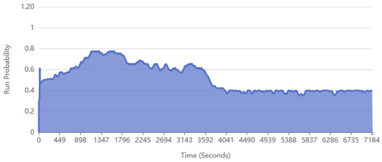
Figure 6.
A plot of the change in run probability of the surveillance camera using elasticity.
Now that all the concepts, categories, and properties that deal with time-related behavior and constraints are explained, the categories that contain basic architectural definitions of software are presented in the following sections.
3.6. Parameters
This category contains properties that describe the data I/O involved in the behavior of the profile; they help us to anticipate the load of data among operations and instances. The ID property assigns the parameter an individual and unique identifier number. The description provides a textual description of what the parameter represents. The direction allows us to define whether the parameter is external or internal. External parameters are parameters that can come from and go to other instances, while internal parameters are parameters used or created by the operations within an instance. The final property available to describe parameters is size. It defines a quantitative amount for the size of the parameter in any desired unit.
3.7. Operations
The operations category contains properties responsible for describing what hardware resources an instance consumes, in compliance with criteria C8. The ID property gives each operation a unique numeric identifier while the description property exists to provide a textual description of what the operation represents.
3.7.1. Operation Resource Usage
The resource usage category defines quantitative amounts of consumption per hardware resource per operation. It allows us to satisfy C9, as resource usage is tightly related to energy consumption. Since software and hardware energy consumption metrics can vary from one method to another, there is no specific metric that we apply to resource usage. However, as previous authors have noted [34], a multitude of relevant metrics can be used to describe hardware and software performance or hardware consumption.
3.7.2. Operational Time Constraints
Operational time constraints consist of the same properties and mechanics as run constraints. The main difference is what run time means to the operation. Run time, from the point of view of the operation, is operational time, which means that the maximum and minimum limits of the operational time are bounded within the instance’s run time. The Quota property bounds the maximum operational time per instant run and the Cooldown property declares the time to wait before the operation is available again within the same instant run time of an instance.
3.7.3. Operational Dependencies
The pair of properties in this category describes the relationships among operations. The first property is the Target ID, whose value defines the unique identifier number of the target operation to establish a relationship with. The dependency type property offers two types of relationships to choose from: dependee and dependent. If dependee is chosen, the target would depend on the operation being defined. The inverse occurs when dependent is selected as the type of relationship. It is important to keep in mind that an instance with both of its states’ probabilities set to 0 will only run if an operational dependency is triggered.
3.7.4. Results
The properties in this category create a relationship among operations through parameters, complying with C3 and C4. The first property, parameter ID, corresponds to the identifier number of a parameter. Its purpose is to identify the parameter the operation will output when executed. The next property is the Operation ID, which defines to which operation the result will be “sent”. In this way, we can chain operations together.
Now that we have defined two levels of dependency management for operations, there is a final level that lets us clarify exactly what activates them: the triggers set.
3.7.5. Triggers
As the name implies, triggers are responsible for the initiation of an operation in compliance with C3. The type property defines if the trigger for the operation will be a parameter or a state change. To define exactly which parameter or state will trigger the operation, the trigger’s parameter ID (row 25 of Table A2) is considered. If the type is set to a state, the possible values for the ID become either run or stop. If the type is set to a parameter, the ID of the corresponding parameter must be entered.
4. Integrative Example
To provide an example that demonstrates a realistic use case for our BBCP, we analyzed an existing application from the perspective of a black-box service-oriented architecture (SOA), and created a couple of BBCPs to simulate its behavior. The application in question, GeForce Now, is a cloud gaming service developed by NVIDIA [35], which we chose due to the popularity of streaming platforms and, more specifically, the human–computer interaction involved in cloud gaming. In cloud gaming, the hardware responsible for running the game and managing inputs and outputs from and to the consumer is in the cloud (a computer cluster in the network), making use of the software-as-a-service delivery model (SaaS) based on subscriptions.
In contrast to other streaming services such as video streaming, the user provides intermittent hardware peripheral input such as mouse movement and keyboard strokes to the cloud over the internet. The user’s input is then processed and reacted upon by the game in the cloud, resulting in subsequent video and audio sent over the internet to the user. From a SOA perspective, there are two self-contained functions (services) that we have profiles: the Catalog Service and the Game Stream Service.
The Catalog Service is responsible for offering the user a menu of the games available to play, usually by employing recommendation algorithms that cater the content to the preferences of the user. Once a game is selected from the menu, the Game Stream Service is responsible for the rest of the I/O operations between the cloud and the user, until the user decides to stop playing the game. The objective of this example is to obtain an estimation of the energy consumption of the Game Stream Service using BBCP in combination with the time constraints that the subscription service employs to limit the play time of a user demoing it.
4.1. The Catalog Service
For our game stream profile to work, we characterized a BBCP with the information from the Catalog Service. We gave the profile a deliberate Profile Evaluation Rate (PER) equal to 1/600 Hz (an evaluation every 10 min). The run and stop probabilities were set equally to 0.5 to establish an unbiased baseline. We set the scale to 7 to simulate a week, and created two cycles. The first cycle takes place during the weekdays (Monday through Friday) when the service’s customers’ spare time is reduced, while the second cycle takes place during the weekends when game streaming services are used the most due to the increase in the available time of its customers.
To complement the cycles, we created three timed expectations for each of them, available in Table 4, which are meant to divide the day in three different time segments: work time, spare time, and nighttime. The behavior was further constrained using elasticity for each timed expectation.
Table 4.
Catalog Service: timed expectations per cycle.
The values used for the elasticity of each timed expectation are available in Table 5. We concluded the characterization of the Catalog Service expectations by adding run constraints to each timed expectation (see Table 6) to simulate the deliberate time restrictions that the users demoing the product would encounter. A Minimum Run Time equal to 0 stands for no minimum threshold of time running. Such limitations are usually set in place by subscription business models to entice the user to become a member, removing these restrictions. As seen in the timed expectations for both cycles, the execution probability tends to increase into the latter part of the day, as well as the minimum and maximum time of consumption. This is due to the amount of spare time a user tends to have for this type of application, common across leisure activities.
Table 5.
Catalog Service: elasticity constraints per timed expectation.
Table 6.
Catalog Service: run constraints per timed expectation per cycle.
For this profile, we decided to add a single operation with no actual resource consumption or operational time constraints, available in Table 7. The goal of this operation was to define an operational trace between the Catalog Service and the Game Stream Service, where the catalog selection functions as a trigger for the Game Stream Service each time it runs. This relationship will become more evident further on with the definition of the Game Stream Service in Section 4.2.
Table 7.
Catalog Service: the description, triggers, and results of operation 1.
4.2. The Game Stream Service
The PER of this profile was set to 60, as video games usually maintain a frame rate of around 30 to 60 FPS (images or frames per second) to reflect the quality of service (the perceived quality by the user) that these types of applications strive for [36]. Our Default Run Probability was set to 0 and our stop probability to 0 because the instance of this profile is always triggered by one of its operations. The parameters, available in Table 8, have a size relative to the network requirement of the application: 25 Mbits/second or 0.00468 MB per millisecond. When the parameters’ direction is set to “external”, they can be accounted for as network consumption, reducing the need for creating more profiles.
Table 8.
Catalog and Game Stream Services: parameters to use.
The operations in this profile, as defined in Table 9, hold a circular relationship among them. This results in the operational loop illustrated in the diagram of Figure 7, where the parameters, triggers, and results match the definitions above. In addition to this, we set a maximum and minimum amount of time the operations can be sustained (in seconds) in compliance with the time constraints of the business model.
Table 9.
Game Stream Service: its operations (a), the relationships across its operations (b), the triggers per operation (c), the results of each operation (d), and, finally, the time constraints per operation (e).
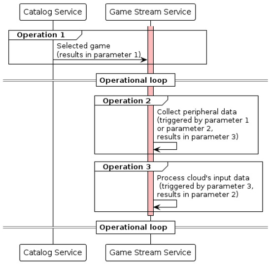
Figure 7.
Sequence diagram showing the interactions between the Catalog Service and the Game Stream Service.
To conclude the modeling of the Game Stream Service, we populated the operations with hardware consumption values, a fundamental part of the BBCP. The values were taken from the official system requirements found on the application’s webpage (https://www.nvidia.com/en-eu/geforce-now/system-reqs/, accessed on 2 August 2024), considering 60 frames per second at a 1080 p image resolution as our target performance and a computer with Windows as the consumer platform. The storage consumption was excluded, as it does not appear to have a minimal requirement during run time.
To assign the consumption values to each one of the operations, we decided to distribute one-third of the consumption to the peripheral data recollection operation. The remaining two-thirds are assigned to the frame and audio rendering operation. This was decided due to the high importance of the latter, as video processing is usually a taxing process. The values used for each operation are available in Table 10.
Table 10.
Game Stream Service: resource usage per operation.
4.3. Methodology of Testing and Results
To validate our approach, we created a system design of the interpreter, constituted by the properties and the values in the example as well as their pertaining logic. The simulator we chose to model our system is Insight Maker, a “general-purpose web-based simulation and modeling tool” [37]. We chose Insight Maker due to its low learning curve, high flexibility, collaborative features, support of system dynamics as well as agent-based modeling and, last but not least, free and open-source nature. With it, we portrayed each of the elements of the BBCP as variables, and the underlying logic to interpret them as separate state machines.
The Catalog Service and Game Stream Service models created with Insight Maker are accessible through our website [33]. For clarity, we decided to create a separate model for each service. As the Game Stream Service maintains an operational loop, a simulation that uses the accumulated run time of the Catalog Service as a direct input for the Game Stream Service to use as the operational time was enough. The equations and hardware specifications to obtain the energy consumption of the service were taken from various sources, such as Intel datasheets and official network device standards. The equations employed per hardware resource are available in Table 11, and the variables and values we used are available in Table 12.
Table 11.
Equations used to estimate the energy consumption of the hypothetical hardware usage of the BBCP.
Table 12.
Hypothetical hardware values used to estimate energy consumption.
We performed three experiments: one that sampled the energy consumption of the first cycle of the game stream profile for a day and a second one that sampled the energy consumption of its second cycle for a day. In the third experiment, we sampled an hour of the second experiment during its third definition of timed expectations, using an agent simulation of 50 agents. In the context of Insight Maker and our interpreter, an agent is a dynamic representation of a BBCP; in other words, 50 instances of a BBCP were used. The steps we followed in executing our first two experiments were the following:
- We executed a simulation of the first cycle of the Catalog Service with a duration of a day.
- We executed a simulation of the first cycle of the Game Stream Service using the accumulated run time of our first experiment as an input, sampling the behavior over a single day.
- We repeated the previous steps using the data of the second cycle for each profile.
Our two criteria for experimental success were the following:
- A quantitative approximation of the energy consumption should be obtained to demonstrate that energy consumption can be drawn from the simulation of behavioral profiles.
- Both of the cycles defined above should be simulated and contrasted to understand how the re-definition of behavior affects the consumption of hardware and, in the end, energy consumption.
By using our BBCP and the test engine in Insight Maker, we estimated an energy consumption of 127,700.10 Joules over 14,403 s generated by the Game Stream Service during the first experiment (the first cycle). With this result, we satisfy the first requisite for validating our approach, demonstrating that a quantitative approximation of energy consumption can be obtained by instancing our profiles.
In the second experiment, a total energy consumption of 271,296.22 Joules over an operational time of 28,801 s were obtained using the BBCP approach. To conclude our first two experiments, we contrasted the results of the first cycle against those of the second cycle. The data are available in Table 13. The energy expenditure during the second cycle of the Game Stream Service BBCP results in an increment of 143,596.12 Joules and an increase of operational time equal of 14,403 s.
Table 13.
Game Stream Service: the difference in energy consumption between the first and the second cycles.
To provide a comparison of our approach against the real energy consumption of the GeForce Now client’s side, we set up a test bed and recorded the hardware consumption of GeForce Now for the same duration as the first and then the second experiments, using PowerJoular to obtain the power draw [41] of the CPU for each one. The hardware specifications used to calculate the RAM and network card energy consumption in the test bed can be found in Table 14, and a comparative table of the results of the test bed against the ones of the BBCP simulation is available in Table 15.
Table 14.
Hardware specifications of the test bed used to obtain the actual power draw of Geforce Now.
Table 15.
The difference in the estimated energy consumption of the experiments against the energy measurements obtained from our test bed.
The steps of the third experiment diverged from the previous ones in the following ways:
- We cloned the Insight Maker model and the values used in the second experiment and re-configured it to an agent simulation.
- We set the beginning of the experiment to the third timed expectation (row 3 of Table 4), and a total duration of 3600 s for the simulation. The duration was decided after the previously observed performance issues of Insight Maker in longer simulations caused the simulator to encounter a memory error.
- We reduced the Minimum Run Time to 300 s (5 min) so that agents would not spend most of the brief simulation in a run state.
The evolution in the number of agents running throughout the third experiment can be seen in Figure 8. In addition, the sum of the run time and the projected energy expenditure of its agents are available in Table 16.
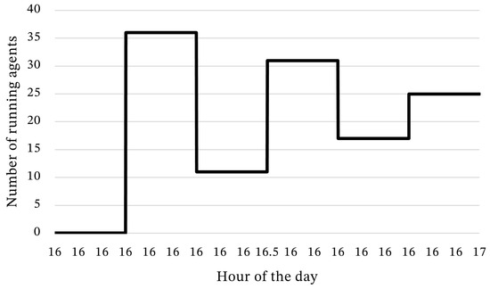
Figure 8.
Amount of agents running throughout the third experiment.
Table 16.
The overall projected energy expenditure and run time of the agent simulation.
5. Lessons Learnt
We drew the following conclusions out of our experiments:
- It is possible to approximate the behavior and consumption of pre-existing software with the BBCP. In addition, behavior can be easily modified.
- Elasticity ensures that user satisfaction can be accounted for and that business constraints related to time, such as usage time constraints, can also be easily adjusted and enforced throughout different time periods.
- Refining and constraining profiles with a deeper analysis of their prospective user base allows for a more accurate simulation of the potential hardware load.
- The differences between the results of the BBCP models and the test bed in Table 15 were due to hardware specifications that can be easily replicated in the BBCP, such as the double ram consumption or the variability in CPU consumption. However, the culprit of the variability in CPU consumption seems to be Google Chrome, which was used as the host program for GeForce Now.
- The BBCP approach allows us to estimate energy consumption in scenarios that could be difficult to replicate. For example, the multi-agent simulation allows software architects to obtain stress test data that accounts for user behavior and business rules without setting up a hardware cluster, requiring the actual software, or conducting a massive user testing effort.
The previous examples demonstrate that developing a BBCP just requires a reduced amount of knowledge of software architecture, an approximation or, at least, an example of the resources that each operation will consume, and a general idea of the user behavior over time. We envision the BBCP as an approach that could be incorporated (initially) during the analysis and conception phases of the software development life cycle. For instance, in sequential and parallel methodologies, such as the Waterfall and V-model, the integration of the BBCP into the modeling (analysis and design) stages can be a part of the requirement process. Since UML is often used during these stages, the relevant BBCP profiles can be developed using the same project knowledge base, adding minimal overhead.
During the development (or construction) phase, the BBCP aspects like expected hardware consumption, timing expectations, and volatile behaviors (e.g., sensor-related triggers) can help developers prioritize code efficiency, particularly in operations that are the most resource-intensive. This prioritization can lead to reduced hardware consumption in the final product. In the deployment stage, the BBCP can contribute to more efficient deployments by using its insights into hardware load. This allows teams to prepare deployments with appropriate scheduling algorithms, infrastructure, or other strategies, especially beneficial in parallel methodologies, where deployment planning could begin concurrently with analysis and design. Incremental and iterative methodologies would also perceive the same benefits.
For evolutionary methodologies such as Agile, where quick results often take precedence over detailed documentation, the BBCP can be leveraged as an early deliverable rather than just being part of the documentation. The interpreter’s output can provide developers with predictions on software behavior changes, enabling them to adapt more swiftly and potentially reduce development time. Finally, the estimation of its energy consumption could provide full-stack green software development methodologies, such as the one proposed in [42], a continuous support where the BBCPs created during the analysis and design phases are carried on and re-assessed at each step of the software development, until obtaining a final classification of the software and the profile according to its energy consumption. This, in turn, will transform our BBCP into an exchangeable format of behavior and energy consumption that enables systems to adapt to frugal configurations preemptively. We elaborate further on how the BBCP can be adopted in a software development methodology in Appendix A.
6. Conclusions and Future Work
In this article we proposed our behavior-based consumption profiles, a DSL specialized in the description of the evolution of stochastic software behavior and behavior with software, aimed at producing estimations of prospective energy consumption. Unlike other approaches, the flexibility of our method makes it hardware- and software-platform-agnostic. This allows software designers to focus on a behavior-first approach without worrying about technical details. In addition, our proposal facilitates the description of external constraints that affect software consumption, such as HCI, business constraints, and even hypothetical hardware sensors. We also explained its elements, characteristics, and mechanics, and provided an integrative example where we analyzed and profiled a real-world video game streaming service. We believe that our approach is a key step towards greener software and systems design and architecture that aid software designers and developers in profiling software’s behavioral consumption without a lot of technicalities. We are aware that the profiling process would benefit from a tool that guides its users through each component of the BBCP, and improves over the performance of Insight Maker during multi-agents simulations. As future work, we will develop and publish a Computer-Assisted Software Engineering (CASE) tool that incorporates the proposed DSL and the experimental interpreter used for the experiments in this article into the software architecture process during the analysis and design stages of the SDLC.
Author Contributions
Conceptualization, J.A.L., S.I. and P.R.; methodology, J.A.L., S.I. and P.R.; software, J.A.L.; validation, J.A.L.; investigation, J.A.L.; data curation, J.A.L.; writing—original draft preparation, J.A.L.; writing—review and editing, J.A.L., S.I. and P.R.; visualization, J.A.L.; supervision, S.I. and P.R.; project administration, J.A.L., S.I. (coordinator of the NEAT-AMBIENCE project) and P.R.; funding acquisition, S.I. and P.R. All authors have read and agreed to the published version of the manuscript.
Funding
This publication is part of the PID2020-113037RB-I00 project, funded by MICIU/AEI/10.13039/501100011033.
Data Availability Statement
The original data presented in the study are openly available in [33].
Acknowledgments
Besides the NEAT AMBIENCE project, we also acknowledge the support of the Departamento de Ciencia, Universidad y Sociedad del Conocimiento del Gobierno de Aragón (Government of Aragon: Group Reference T64_23R, COSMOS research group).
Conflicts of Interest
The authors declare no conflicts of interest.The funders had no role in the design of the study; in the collection, analyses, or interpretation of data; in the writing of the manuscript; or in the decision to publish the results.
Appendix A. Integrating the BBCP as a Design Method
To ease the adoption of the BBCP, and give users a frame of reference for the development of profiles, we prepared the BBCP Development Index. The BBCP Development Index, available in Table A1, is a table that proposes three levels of development maturity, where level 1 is the least mature and 3 is the most mature. We limited the index to three levels to facilitate its comprehension. Each level consists of the following items:
- A description of the pre-requirements for each level.
- A description of the process to achieve the target level.
- The expected outcomes of the level.
Our proposal to incorporate our BBCP into the multiple stages of a GSD method is the following:
- Introduce the BBCP to software designers and architects in the design stages of the project, resulting in the following:
- (a)
- A description of behavior, expected hardware consumption, and functional dependencies, at the individual function level.
- (b)
- The dependencies management among components and an expectation of component hardware consumption, at the component level.
These are later passed on to the DevOps (development and operations) team. - The DevOps team uses the results of the design stage to achieve the following:
- (a)
- Identify and implement the best practices in the code and technology stack, in addition to other tools for testing the prototype’s consumption.
- (b)
- Swiftly re-adjust the BBCP to categorize the actual hardware consumption of the prototype.
- (c)
- Employ our custom interpreter to generate the estimated prospective usage data based on the adjusted software models.
- The DevOps team uses the prospective usage data of the profiles to achieve the following:
- (a)
- Create proactive orchestration algorithms that account for the evolution of hardware usage throughout time using re-deployment simulators like PISCO [43].
- (b)
- Obtain information about the prospective consumption of their stack at the deployment level with tools such as Cloud Carbon [44] or Green Cost Explorer [45].
- (c)
- Re-adjust the configuration of the technology stack for the final deployment.
Any of the previous steps proposed can be revisited to accommodate new changes that contribute to more frugal software. We envision the BBCP as a tool to model the first-order and third-order effects of the usage stage of the GREENSOFT model [7] during the design stage of the SDLC. The first-order and third-order effects proposed by the GREENSOFT model include, but are not limited to the following:
- Rebound effects;
- Change of business processes or goals;
- Software-induced hardware consumption;
- Software-induced energy consumption;
- Hardware requirements.
Table A1.
The BBCP development maturity levels.
Table A1.
The BBCP development maturity levels.
| Level | Pre-Requirements | Description | Expected Outcomes |
|---|---|---|---|
| 1 |
| This is the initial level, where the designers and/or architects of the software analyze the requirements stated by the stakeholders of the project and create an initial architecture with it. You can follow the following steps:
| It is expected that your BBCPs have, as a bare minimum, the following:
|
| 2 | Everything in level 1, plus the following:
| At this level, the core features of the BBCP are applied:
| It is expected that your BBCPs have, as a bare minimum, the following:
|
| 3 | Everything in level 2, plus the following:
| At this level, the advanced features of the BBCP are applied:
| It is expected that your BBCPs have, as a bare minimum, the following:
|
Appendix B. Building Correct BBCPs
It is crucial to ensure that the schema provided with the BBCP [33] is correctly utilized. This means that, when creating objects within a category, they should be placed within the appropriate array. For instance, if the user were to declare two operations in the “Operations” category, they would need to create two new JSON object literals, each containing a copy of their respective properties and sub-categories, as demonstrated in Algorithm 1. In addition to the correct creation of objects, it is important to be wary of the constraints involved in the logical nesting of certain categories, such as expectations. Expectations contain cycles and events, which, at the same time, contain timed expectations. It is crucial for timed expectations to always be within a cycle or an event. Furthermore, it is mandatory to provide each object literal with a copy of all the properties that correspond to it, even if none of them will be used. An example of timed expectations can be found in Algorithm 2. Finally, we have prepared Table A2 to guarantee that the values per property available in the BBCP are correct by providing a possible value, type, and format for each one.
| Algorithm 1: Creating multiple operations in the corresponding category |
|
| Algorithm 2: Creating timed expectations within its parent object |
|
Table A2.
Properties in the BBCP, their type, and possible values.
Table A2.
Properties in the BBCP, their type, and possible values.
| Row | Name | Numeric | Text | Bounds | Boolean | Possible Values |
|---|---|---|---|---|---|---|
| 1 | Profile Evaluation Rate | x | Hz | |||
| 2 | Default Run Probability | x | ||||
| 3 | Default Stop Probability | x | ||||
| 4 | Minimum Run Time | x | ; if the property will be ignored. | |||
| 5 | Maximum Run Time | x | ; if the property will be ignored. | |||
| 6 | Quota | x | ; if the property will be ignored. | |||
| 7 | Cooldown | x | ; if the property will be ignored. | |||
| 8 | Countdown | x | ; if the property will be ignored. | |||
| 9 | Days | x | Ranges: [1–7], selections: [1, 3, 6], selections and ranges: [1–3, 6] (the values are just for demonstration) | |||
| 10 | Scale | x | the interpreter’s duration | |||
| 11 | Initial Day | x | ; if the property will be ignored. | |||
| 12 | End Day | x | ; if the property will be ignored. | |||
| 13 | Time Range | x | Ranges: [1–12], selections:[3, 17], selections and ranges: [1–12, 17] | |||
| 14 | Run Probability Override | x | ||||
| 15 | Stop Probability Override | x | ||||
| 16 | Elasticity | x | True or False | |||
| 17 | Minimum Run Probability | x | ; if the property will be ignored. | |||
| 18 | Maximum Run Probability | x | ; if the property will be ignored. | |||
| 19 | Maximum Stop Probability | x | ; if the property will be ignored. | |||
| 20 | Minimum Stop Probability | x | ; if the property will be ignored. | |||
| 21 | Negative Run Probability Modifier | x | ; if the property will be ignored. | |||
| 22 | Negative Stop Probability Modifier | x | ; if the property will be ignored. | |||
| 23 | Positive Run Probability Modifier | x | if the property will be ignored. | |||
| 24 | Positive Stop Probability Modifier | x | if the property will be ignored. | |||
| 25 | Any ID | x | x | for identifier numbers or the name of the state for triggers. | ||
| 26 | Any description | x | Text | |||
| 27 | Any hardware usage | x | ||||
| 28 | Dependency Type | x | Dependee or Dependent | |||
| 29 | Trigger Type | x | Parameter or State | |||
| 30 | Parameter Direction | x | Internal or External | |||
| 31 | Parameter Size | x |
References
- European Environment Agency. Growth without Economic Growth. 2021. Available online: https://www.eea.europa.eu/publications/growth-without-economic-growth (accessed on 2 August 2024).
- Kerschner, C.; Wächter, P.; Nierling, L.; Ehlers, M.H. Degrowth and Technology: Towards Feasible, Viable, Appropriate and Convivial Imaginaries. J. Clean. Prod. 2018, 197, 1619–1636. [Google Scholar] [CrossRef]
- Noman, H.; Mahoto, N.A.; Bhatti, S.; Abosaq, H.A.; Al Reshan, M.S.; Shaikh, A. An Exploratory Study of Software Sustainability at Early Stages of Software Development. Sustainability 2022, 14, 8596. [Google Scholar] [CrossRef]
- Jagroep, E.; Broekman, J.; van der Werf, J.M.E.M.; Brinkkemper, S.; Lago, P.; Blom, L.; van Vliet, R. Awakening awareness on energy consumption in software engineering. In Proceedings of the 39th International Conference on Software Engineering: Software Engineering in Society Track, Buenos Aires, Argentina, 20–28 May 2017; (ICSE-SEIS). pp. 76–85. [Google Scholar] [CrossRef]
- García-Berna, J.A.; Carrillo de Gea, J.M.; Moros, B.; Fernández-Alemán, J.L.; Nicolás, J.; Toval, A. Surveying the Environmental and Technical Dimensions of Sustainability in Software Development Companies. Appl. Sci. 2018, 8, 2312. [Google Scholar] [CrossRef]
- Pang, C.; Hindle, A.; Adams, B.; Hassan, A.E. What Do Programmers Know about Software Energy Consumption? IEEE Softw. 2015, 33, 83–89. [Google Scholar] [CrossRef]
- Naumann, S.; Dick, M.; Kern, E.; Johann, T. The GREENSOFT Model: A Reference Model for Green and Sustainable Software and Its Engineering. Sustain. Comput. Inform. Syst. 2011, 1, 294–304. [Google Scholar] [CrossRef]
- Jiménez, A.R.T. Hacia la sostenibilidad energética: Una revisión de literatura del desarrollo de software verde. In Actas del Congreso Internacional de Ingeniería de Sistemas; Universidad de Lima: Lima, Peru, 2023; pp. 43–58. [Google Scholar] [CrossRef]
- Larracoechea, J.; Roose, P.; Ilarri, S.; Cardinale, Y.; Laborie, S.; Vara, O. Behavior-Based Consumption Profiles for the Approximation of the Energy Consumption of Services. In Proceedings of the International Conference on Information Systems Development (ISD), Cluj-Napoca, Romania, 31 August–2 September 2022. [Google Scholar]
- Pierre Bourque, R.E.F. (Ed.) Guide to the Software Engineering Body of Knowledge; IEEE: Piscataway, NJ, USA, 2014. [Google Scholar]
- Butterfield, A.; Ngondi, G.E.; Kerr, A. (Eds.) A Dictionary of Computer Science; Oxford University Press: Oxford, UK, 2016. [Google Scholar]
- SEBoK. Behavior (Glossary). 2022. Available online: https://www.sebokwiki.org/wiki/Behavior_(glossary) (accessed on 2 August 2024).
- Bowring, J.F.; Rehg, J.M.; Harrold, M.J. Software Behavior: Automatic Classification and Its Applications; Technical Report; Georgia Institute of Technology: Atlanta, GA, USA, 2003. [Google Scholar]
- Harzing, A.W. Publish or Perish. 2019. Available online: https://harzing.com/resources/publish-or-perish (accessed on 2 August 2024).
- Psaier, H.; Juszczyk, L.; Skopik, F.; Schall, D.; Dustdar, S. Runtime Behavior Monitoring and Self-Adaptation in Service-Oriented Systems. In Socially Enhanced Services Computing: Modern Models and Algorithms for Distributed Systems; Dustdar, S., Schall, D., Skopik, F., Juszczyk, L., Psaier, H., Eds.; Springer: Berlin/Heidelberg, Germany, 2011; pp. 117–138. [Google Scholar] [CrossRef]
- Zaha, J.M.; Barros, A.; Dumas, M.; ter Hofstede, A. Let us Dance: A Language for Service Behavior Modeling. In Proceedings of the On the Move to Meaningful Internet Systems 2006: CoopIS, DOA, GADA, and ODBASE; Meersman, R., Tari, Z., Eds.; Springer: Berlin/Heidelberg, Germany, 2006; Lecture Notes in Computer Science; pp. 145–162. [Google Scholar] [CrossRef]
- van der Aalst, W.M.P.; Dumas, M.; Ouyang, C.; Rozinat, A.; Verbeek, E. Conformance Checking of Service Behavior. ACM Trans. Internet Technol. 2008, 8, 1–30. [Google Scholar] [CrossRef]
- Östberg, P.O. A Model for Simulation of Application and Resource Behavior in Heterogeneous Distributed Computing Environments. In Proceedings of the 2nd International Conference on Simulation and Modeling Methodologies, Technologies and Applications (SIMULTECH), Rome, Italy, 28–31 July 2012; pp. 144–151. [Google Scholar]
- Kim, J.E.; Kapoor, R.; Herrmann, M.; Haerdtlein, J.; Grzeschniok, F.; Lutz, P. Software Behavior Description of Real-Time Embedded Systems in Component Based Software Development. In Proceedings of the 2008 11th IEEE International Symposium on Object and Component-Oriented Real-Time Distributed Computing (ISORC), Orlando, FL, USA, 5–7 May 2008; pp. 307–311. [Google Scholar] [CrossRef]
- Niu, X.; Liu, H.; Xin, G.; Huang, J.; Li, B. User Application Behavior Sequence Generation. In Proceedings of the 2020 IEEE International Conference on Advances in Electrical Engineering and Computer Applications (AEECA), Dalian, China, 25–27 August 2020; pp. 466–469. [Google Scholar] [CrossRef]
- Rosenthal, C.; Congdon, C.B. Personality Profiles for Generating Believable Bot Behaviors. In Proceedings of the 2012 IEEE Conference on Computational Intelligence and Games (CIG), Granada, Spain, 11–14 September 2012; pp. 124–131. [Google Scholar] [CrossRef]
- Koskinen, J.; Kettunen, M.; Systä, T. Behavioral Profiles-a Way to Model and Validate Program Behavior. Softw. Pract. Exp. 2010, 40, 701–733. [Google Scholar] [CrossRef]
- Corrales, J.C.; Grigori, D.; Bouzeghoub, M.; Burbano, J.E. BeMatch: A Platform for Matchmaking Service Behavior Models. In Proceedings of the 11th International Conference on Extending Database Technology: Advances in Database Technology (EDBT), Nantes, France, 25–29 March 2008; Association for Computing Machinery: New York, NY, USA; pp. 695–699. [Google Scholar] [CrossRef]
- Gaaloul, W.; Bhiri, S.; Rouached, M. Event-Based Design and Runtime Verification of Composite Service Transactional Behavior. IEEE Trans. Serv. Comput. 2010, 3, 32–45. [Google Scholar] [CrossRef]
- Vasudevan, M.; Tian, Y.C.; Tang, M.; Kozan, E. Profile-Based Application Assignment for Greener and More Energy-Efficient Data Centers. Future Gener. Comput. Syst. 2017, 67, 94–108. [Google Scholar] [CrossRef]
- Ponsard, C.; Deprez, J.C. A UML KPI Profile for Energy Aware Design and Monitoring of Cloud Services. In Proceedings of the 2015 10th International Joint Conference on Software Technologies (ICSOFT), Colmar, France, 20–22 July 2015; Volume 1, pp. 1–6. [Google Scholar]
- Shorin, D.; Zimmermann, A. Evaluation of Embedded System Energy Usage with Extended UML Models. In Softwaretechnik-Trends; Springer: Berlin/Heidelberg, Germany, 2013; pp. 16–17. [Google Scholar] [CrossRef]
- Benton, S.; Altemeyer, B.; Manning, B. Behavioural Prototyping: Making Interactive and Intelligent Systems Meaningful for the User. In Proceedings of the 2010 International Conference on Intelligent Networking and Collaborative Systems (INCoS), Thessaloniki, Greece, 24–26 November 2010; pp. 319–322. [Google Scholar] [CrossRef]
- The Object Management Group®. OMG MARTE | Object Management Group. Available online: https://www.omg.org/omgmarte/ (accessed on 2 August 2024).
- Schall, D.; Truong, H.L.; Dustdar, S. Unifying Human and Software Services in Web-Scale Collaborations. Internet Comput. IEEE 2008, 12, 62–68. [Google Scholar] [CrossRef]
- Holanda, H.J.A.; Marques, C.K.d.M.; Pinto, F.A.P.; Guéhéneuc, Y.G. BPEL4PEOPLE Anti-Patterns: Discovering Authorization Constraint Anti-Patterns in Web Services. In Proceedings of the Anais do Workshop sobre Aspectos Sociais, Humanos e Econômicos de Software (WASHES), Porto Alegre, Brasil, 22–26 July 2018. [Google Scholar] [CrossRef]
- Claude, G. Encyclopedia of Human Computer Interaction; Idea Group Inc. (IGI): Hershey, PA, USA, 2005. [Google Scholar]
- Universidad de Zaragoza; University of Pau. Behavior Based Consumption Profiles (BBCP). 2024. Available online: https://github.com/silarri/BBCP (accessed on 28 July 2024).
- Guldner, A.; Bender, R.; Calero, C.; Fernando, G.S.; Funke, M.; Gröger, J.; Hilty, L.M.; Hörnschemeyer, J.; Hoffmann, G.D.; Junger, D.; et al. Development and Evaluation of a Reference Measurement Model for Assessing the Resource and Energy Efficiency of Software Products and Components—Green Software Measurement Model (GSMM). Future Gener. Comput. Syst. 2024, 155, 402–418. [Google Scholar] [CrossRef]
- GeForce NOW Cloud Gaming. Available online: https://www.nvidia.com/en-us/geforce-now/ (accessed on 2 August 2024).
- Di Domenico, A.; Perna, G.; Trevisan, M.; Vassio, L.; Giordano, D. A network analysis on cloud gaming: Stadia, GeForce Now and PSNow. Network 2021, 1, 247–260. [Google Scholar] [CrossRef]
- Fortmann-Roe, S. Insight Maker: A General-Purpose Tool for Web-Based Modeling & Simulation. Simul. Model. Pract. Theory 2014, 47, 28–45. [Google Scholar] [CrossRef]
- Intel. Enhanced Intel SpeedStep Technology for the Intel Pentium M Processor; Technical Report; Intel: Santa Clara, CA, USA, 2004. [Google Scholar]
- Valera, H.H.A.; Dalmau, M.; Roose, P.; Larracoechea, J.; Herzog, C. An Energy Saving Approach: Understanding Microservices as Multidimensional Entities in P2P Networks. In Proceedings of the 36th Annual ACM Symposium on Applied Computing (SAC), Virtual, 22–26 March 2021; Association for Computing Machinery: New York, NY, USA, 2021; pp. 69–78. [Google Scholar]
- Chiaravalloti, S.; Idzikowski, F.; Budzisz, Ł. Power Consumption of WLAN Network Elements; Technical University Berlin: Berlin, Germany, 2011. [Google Scholar] [CrossRef]
- Noureddine, A. PowerJoular and JoularJX: Multi-Platform Software Power Monitoring Tools. In Proceedings of the 18th International Conference on Intelligent Environments (IE2022), Biarritz, France, 20–23 June 2022. [Google Scholar]
- Roose, P.; Sergio, I.; Larracoechea, J.A.; Cardinale, Y.; Laborie, S. Towards an Integrated Full-Stack Green Software Development Methodology. In Proceedings of the 29th International Conference on Information Systems Development, Valencia, Spain, 8–10 September 2021. [Google Scholar]
- Humberto Alvarez Valera, H.; Dalmau, M.; Roose, P.; Larracoechea, J.; Herzog, C. PISCO: A Smart Simulator to Deploy Energy Saving Methods in Microservices Based Networks. In Proceedings of the 2022 18th International Conference on Intelligent Environments (IE), Biarritz, France, 20–23 June 2022; pp. 1–4. [Google Scholar] [CrossRef]
- Cloud Carbon Footprint. Available online: https://www.cloudcarbonfootprint.org/ (accessed on 2 August 2024).
- The Green Web Foundation/Green-Cost-Explorer. Available online: https://github.com/thegreenwebfoundation/green-cost-explorer (accessed on 2 August 2024).


Disclaimer/Publisher’s Note: The statements, opinions and data contained in all publications are solely those of the individual author(s) and contributor(s) and not of MDPI and/or the editor(s). MDPI and/or the editor(s) disclaim responsibility for any injury to people or property resulting from any ideas, methods, instructions or products referred to in the content. |
© 2024 by the authors. Licensee MDPI, Basel, Switzerland. This article is an open access article distributed under the terms and conditions of the Creative Commons Attribution (CC BY) license (https://creativecommons.org/licenses/by/4.0/).