Techno-Economic Assessment of Coaxial HTS HVAC Transmission Cables with Critical Current Grading between Phases Using the OSCaR Tool

Abstract

In recent years, the scientific and industrial interest regarding alternative technologies for transmission cables has increased. These conductors should efficiently transmit significant amounts of power between grid nodes, which are expected to be particularly congested due to the projected global increase in electricity production. Superconducting cables are considered a promising solution in this context, offering the potential to transmit large amounts of energy with minimal losses and compact dimensions, thereby potentially benefiting the environment. To evaluate the feasibility of integrating superconducting cables into existing grids, techno-economic approaches should be adopted. Such techniques enable the conceptual design of a specific cable structure, allowing users to explore a wide range of operating parameters to derive optimal designs. This paper reports a comprehensive techno-economic analysis of High Voltage Alternating Current (HVAC) cables realized with High-Temperature Superconducting (HTS) tapes, with the aim to transmit extremely high-power level. The optimal coaxial design is selected using Optimization Tool for Superconducting Cable Research (OSCaR) by implementing a graded approach to the critical current of the HTS tapes used for the different phases. This optimization aims to achieve the most effective balance between the cost of the coated conductors and their electrical properties. The whole set of model equations, the user-defined parameters, and the applied constraints are detailed. The OSCaR tool is then applied to assess the impact on the optimized design of the cable system and the corresponding cost indexes of several crucial parameters, such as the maximum transmitted power, the voltage level, and the line length.

1. Introduction

The most notable property of superconducting materials is their ability to carry significantly higher current densities compared with conventional conductors with minimal losses when working at specific operating conditions. Therefore, it is not surprising that their application to the manufacturing of high-power transmission cables was proposed already in the 1960s [1,2]. The application field was limited by the required stringent operating conditions of low-temperature superconductors, especially in terms of cryogenic temperatures. Indeed, scientific and industrial interests surged after the introduction of High-Temperature Superconductors (HTSs), which can markedly reduce the complexity of the cooling system of superconducting cables. Over the last 20 years, this has given rise to a series of public and private projects for the design and realization of small-length prototypes of HTS cables, with the aim of also enabling their future adoption for power transmission over long distances. These projects are distributed worldwide, with notable implementations in South Korea [3,4,5,6], Japan [7,8,9], China [10,11], Europe [12,13,14,15,16], and the USA [17,18]. In fact, with the foreseen increase in global electricity production over the next few years, grids are expected to face significant congestion, requiring efficient power transmission systems for which advancements in superconducting technologies could provide a valid solution.

In this context, various cable designs have been proposed. For example, superconducting cables can be distinguished by considering the mutual position of the electrical insulation and the coolant flow between warm dielectric (insulation placed outside the channel for the cryogenic fluid) and cold dielectric (CD) cables (with insulation contained inside of the cryostat, operating at cryogenic temperatures) [19]. Almost all cable projects proposed nowadays are based on the CD layout as it allows easier access to the cryostat, being electrically insulated from the conductive phases. Furthermore, with reference to AC cables, different configurations can be identified based on the arrangement of the phases and the cryostat. Single-core cables have dedicated cryostats for each of the three phases, while in three-in-one cables, the tapes belonging to each phase are helically wound on three separate axes, and then the phases are contained in a single cryostat. Finally, coaxial cables present the three phases helically co-wound on the same axis and separated by concentric insulating layers [20]. These configurations may be more or less suitable, depending on the operational constraints of the case study. Since no existing production standards for superconducting cables have been established yet, all cable layouts proposed in the literature should be carefully considered in the design phase of new lines or when replacing existing ones.

For HTS cable technology to gain extensive acceptance in national and international grids, it is necessary to determine the possible conditions for technological and economic advantages over conventional solutions. However, the literature presents few comparisons between superconducting and conventional lines. These are limited to specific case studies [21,22,23,24,25], with cable design optimizations not following cost-effectiveness criteria [26,27,28] and focusing on single aspects like losses [29,30,31,32], fluid dynamics [33], or phase balance [34], frequently neglecting some elements of a cable system. On the other hand, cable manufacturers, researchers, and grid operator would all benefit from a comprehensive methodology for designing conductors, even if only at a conceptual level. This procedure should optimize the device design from both technical and economic points of view while considering all cable system components across various operating conditions, line characteristics, and specific constraints. A possible approach is to use the Optimization Tool for Superconducting Cable Research (OSCaR) [35]. This tool allows performing techno-economic analyses of superconducting transmission lines while considering a wide range of operating conditions, facilitating extensive parametric studies, and enabling the identification of cost-effective conductor designs. The tool was originally proposed in [36] for medium-voltage AC HTS coaxial cables cooled with liquid nitrogen (LN₂), but this method can be easily adapted to other configurations, such as MgB₂ DC cables cooled with helium gas [37]. Focusing on a single cable design at a time simplifies both the exposure of the methodology and the resulting output, enhancing their clarity and accessibility for readers.

This work investigates the applicability of the OSCaR approach to HVAC coaxial cables wound using HTS-coated conductors. Conventionally, the coaxial configuration is limited to medium-voltage applications due to the need to incorporate thick concentric insulating layers, but the authors considered it worth exploring its use for HVAC lines, as the design can still be quite compact compared with conventional solutions. Indeed, this configuration offers several advantages compared with other CD layout alternatives. Notably, the concentric design practically cancels the external magnetic field outside of the conductor without requiring a superconducting shield layer or the purchase of additional land near the installation site to mitigate magnetic field limitations imposed by regulations. Regarding the voltage level, power grids are increasingly adopting high-voltage or extra high-voltage (above 220 kV) infrastructures for efficiently transferring electricity from remote renewable energy sources locations to urban centers due to minimal energy loss. Superconducting high-voltage lines present a promising alternative for managing extremely high power levels (in the GW range) over long distances at relatively lower voltage levels (up to 220 kV), simplifying the design, management, and safety. Transferring the same amounts of power using superconducting cables at low or medium voltages would require employing large quantities of expensive tape or operating at temperatures significantly colder than LN₂, both of which pose challenges.

The methodology reported in [35,36] is revised and improved here for HTS HVAC coaxial cables. To the authors’ knowledge, no standardized structure exists for superconducting coaxial cables, known to be produced by manufacturers such as Southwire Company and Nexans. Therefore, its conceptual design was adjusted based on what the authors considered the most reliable guidance from the literature. Section 2, Section 3, Section 4, Section 5 and Section 6 will describe the complete optimization procedure, highlighting the key modifications made to the original code and covering the approach’s overview and the implemented cost, loss, and constraint functions. Notably, an innovative approach with potential application to other superconducting devices is presented in Section 2.2. This focuses on optimizing the quality of the HTS tape used in each of the three AC phases, referred to here as grading of the critical current of the tapes among the phases. In fact, previous modeling revealed an “inconvenient” underloading of certain conductive layers made of high-quality and expensive tapes, with operating currents well below their critical current capacity [35]. Then, after presenting the values of all of the input parameters selected for the model in Section 7, Section 8 will focus on the results of some notable parametric analyses carried out with the tool.

2. Methodology Overview

This work is based on the techno-economic approach proposed in [36] and is revised here. The algorithm optimizes the cable’s design on the basis of the selected operating parameters, such as the rated cable power, the voltage level, or the line length. From a mathematical standpoint, the problem involves minimizing a multi-variable function, representing the cable system’s cost, subject to the electric, geometric, and fluid dynamic constraints imposed by the user. The objective function is described in Section 4. The problem variables correspond to the selected individual design elements, affecting all other design parameters which are not directly involved in the optimization process. The solver then identifies the set of variables producing a design which corresponds to the lowest overall system cost. The use of a numerical solver is necessary due to the complex interconnections between the selected variables related to the cable system’s design. These variables are linked in both explicit and implicit ways, making it almost impossible to manually predict the trends of their optimized combinations as a function of the set line parameters. To achieve this, the native MATLAB algorithm ga was adopted, based on genetic algorithms. A key advantage of ga over other solvers is that it can easily handle integer and non-integer variables simultaneously. It is worth noting that genetic algorithms are stochastic methods. Therefore, in practice, the entire solver runs several times, starting from the same initial solution and storing a combination of optimized variables at each iteration. Finally, the solution leading to the lowest cost while complying with all of the imposed constraints is selected.

In the following paragraphs, the structures of the cable conductor and the whole cable system adopted in this study are presented, followed by descriptions of the system variables selected for the optimization process.

2.1. Cable System Structure Represented in the Tool

Figure 1 shows a sketch of the structure of an AC coaxial cable composed of HTS tapes and considered by the authors in this work. The conductive phases are named 1, 2, and 3 from the innermost to the outermost one. Each phase is composed of a number $n_{l_i }$of HTS tapes co-wound with one of top of the other. The number of tapes wound side by side on each layer is equal to the maximum number which can be accommodated around the circumference given by the inner radius of the HTS layer $R_{i,j}$ and the winding pitch of the layer ${\alpha }_{i,j}$. In the following, the subscript i will indicate the ith phase, and the subscript j will indicate the jth layer within that phase. The layers are numbered progressively from the innermost to the outermost one in a phase.

Then, to describe the structure from the innermost to the outermost coaxial layer, the cable is composed of a central cylindrical and corrugated former, containing a flow of LN₂. The former has an inner radius $R_{f }$and a thickness $t_f$. A leveling layer (not represented in Figure 1) of a thickness $t_{lev}$ is inserted between the former and the first conductive layer to protect the latter against deformation. Subsequently, the tapes composing the first layer of phase 1 are arranged around the circumference $R_{\mathrm{1,1}}$ (in this example, phase 1 → i = 1; layer 1 → j = 1). The thickness of each HTS layer corresponds to the thickness of the selected coated conductor $t_{HTS}$. Eventual additional layers wound on top of the innermost one of the same phase are separated by a Kapton layer of a thickness $t_k$. Then, between the outermost HTS layer of phase 1 and the innermost HTS layer of phase 2, there is a layer of insulating material of a thickness $t_{in{s}_1}$, whose calculation is described in Section 3.5. The first insulating layer separates the conductive phases 1 and 2, the second insulating layer (with a thickness $t_{in{s}_2}$) is between conductive phases 2 and 3, and the third insulating layer (with a thickness $t_{in{s}_3}$) is between conductive phase 3 from the neutral copper layer. Wound around the third insulating layer is a neutral conductor layer with a thickness $t_n$ which is made of copper. A core fixture layer (not represented in Figure 1) with a thickness $t_c$is then arranged around the neutral conductor to ensure mechanical stabilization during cable assembly and operations. Around the described combination of conductive and insulating layers, there is an annular duct with a thickness $t_{an}$ acting as a return channel for the cryogenic fluid. Finally, all of the concentric layers described are contained withing a cryostat with a thickness $t_{cryo}$.

It is worth noting that the values of $t_f$,$t_{lev}$, $t_{HTS }$, $t_k$, $t_n$, $t_c$, and $t_{cryo}$ are set by the user and are not subject to optimization.

The conductor layout we just defined is integrated into the cable system, which additionally includes the cooling system. Figure 2 shows a sketch of the architecture of the cooling system adopted for the cable, called the both-sided cooling option [39]. The line length $L_{line}$ is divided into a series of cable segments included between a couple of cooling stations. Each cable segment consists of two concentric tubes: the former and annular ducts. Both conduits carry the same mass flow of liquid nitrogen ($\dot{m_{LN2}}$) in opposite directions so that it circulates within a closed loop through the cable. A termination cooling station is placed at both sides of the whole cable length; one manages the fluid coming from the former and transfers it into the annular gap, while the other handles the reverse flow. The “left” and “right” labels in Figure 2, as well as the directions of the counterflows in the two ducts, are purely conventional. The function of the cooling stations is to restore the temperature and pressure of the fluid to its original conditions, which have been altered during passage through the preceding cable segment. As will be elaborated upon in Section 6.2, the solver selects the designs complying with the limits on the pressure drop and temperature rise set by the user. In particular, precautions must be taken to prevent a phase transition in the liquid nitrogen, whose boiling could compromise the quality of the heat exchange. For sufficiently long lines, termination cooling stations may not be sufficient to maintain the cryogen within the fluid dynamic constraints. Thus, a number $n_{stat}$ of intermediate cooling stations may be necessary. As illustrated in Figure 2, these intermediate stations must manage both counterflows from the former and the annular gap simultaneously, restoring the initial thermodynamic conditions in both streams. These intermediate stations are assumed to be uniformly spaced at a distance $d_{stat}$, meaning that $d_{stat}=L_{line}/(n_{stat}-1)$. By adopting this simplified hypothesis, the system can be approximated as modular, meaning that each cable segment between adjacent cooling stations is assumed to be identical in design, as well as in the heat produced and then absorbed by the two fluids within that segment. Hence, the optimization can focus on a single cable segment $d_{stat}$ while considering all intermediate cooling stations as equally sized.

2.2. System Variables Selected for the Optimization and Grading Approach

To achieve high computational efficiency, it is advisable to focus on a key subset of variables considered most significant to the cable system’s cost (i.e., the objective function for the solver). This approach facilitates the identification of correlations between these variables and the overall system cost while minimizing the solver’s computational burden. The remaining parameters are either fixed or derived from the system variables, although users can adapt the proposed approach to include them in the optimization for dedicated parametric analyses.

The parameters selected as system variables are highlighted in Figure 1 and Figure 2 as bold terms. These are the inner radius of the former duct $R_f$, the mass flow rate of nitrogen flowing in both the former and the annular duct $\dot{m_{LN2}}$, the number of HTS layers of each phase ${nl}_i$, the winding angle of each HTS layer of each phase ${\alpha }_{i,j}$, the thickness of the annular duct $t_{an}$, the number of intermediate cooling stations $n_{stat}$, and the ratios between the maximum currents flowing in the tapes of the innermost HTS layers of each phase ($\underset{\_}{I_{tap{e}_{i,j}}}$, the sinusoidal current of the tapes in the ith layer of the jth phase) and their corresponding critical current under the most stressful conditions in terms of temperature and magnetic field along a cable segment ($\sqrt{2}\left|\underset{\_}{I_{tap{e}_{i,1}}}\right|/I_c\left(T_{HT{S}_{max}}, {\left|B\right|}_{i,1}, {\theta }_{i,1}\right)$).

The introduction of the last variable changes the approach compared with earlier versions of OSCaR, in which an HTS tape with uniform characteristics was set across all phases. Indeed, it was already observed for medium-voltage coaxial cables [36] that this strategy can result in certain layers exhibiting a rather low ratio between $\underset{\_}{I_{tape}}$ and $I_c$. While not inherently posing operational issues, this scenario implies an “inefficient” expenditure in tape acquisition, wherein tapes with excellent electrical properties might be extremely underloaded. This is particularly true for the outermost phases of the coaxial structure, which require more tapes wound side-by-side around corresponding larger circumferences. The use of high voltages exacerbates this aspect, as thicker layers of insulation are interposed between the phases, leading to much larger circumferences for the outer HTS layers across the conductor cross-section and requiring a corresponding greater number of tapes, while the total phase current remains the same. To overcome this problem, the solver can control the values of $\sqrt{2} \left|\underset{\_}{I_{tap{e}_{i,1}}}\right|/I_c\left(T_{HT{S}_{max}}, {\left|B\right|}_{i,1}, {\theta }_{i,1}\right)$for the three phases, optimizing them within the maximum and minimum limits. While the numerator of the ratio is derived from the operating current and the geometry of the HTS layer using the electrical model described in Section 3.2, the denominator relies on the coated conductor’s characteristic curves, concerning the local temperature and magnetic field conditions. Thus, a dimensionless characteristic function $I_c\left(T_{HTS}, \left|B\right|, \theta \right)$ is implemented in the tool, referring to a selected tape, where the user can freely modify it before running the code. Then, albeit not explicitly, the solver operates on the multiplication factor to apply to this function equivalent to the critical current value at 77 K and the self-field (hereafter called $I_{c_{77 K}}$). Typically, manufacturing companies provide customers with this parameter to characterize their product, often corresponding to the minimum value across the batch length required by the customer. Ensuring high and uniform critical currents across long batches demands great care in the manufacturing process and results in higher costs per unit length for users. Conversely, a customer may require tape supplies with less homogeneous critical currents, still meeting the minimum value criterion along the entire batch length but at a lower cost per unit length. The innovative concept is to let the solver determine the operating ratio for each phase and, consequently, the quality of the tape to be used and its cost per unit length. This selection is further constrained by the maximum and minimum values of $I_{c_{77 K}}$, contingent on the tape’s geometry (e.g., 4 mm- or 12 mm-wide tapes) proposed by the authors based on their sensitivity. This last aspect will be described in Section 6.3.

Notably, each $\sqrt{2} \left|\underset{\_}{I_{tap{e}_{i,1}}}\right|/I_c\left(T_{HT{S}_{max}}, {\left|B\right|}_{i,1}, {\theta }_{i,1}\right)$ratio refers only to the innermost layer of each phase (j = 1), and any additional layer within the same phase utilizes the same type of tape as the one selected for the innermost layer. The authors consider that optimizing the tape quality at the single-layer level would be overly complex in practice. Moreover, the ratio should remain relatively stable across different layers within the same phase.

To the authors’ knowledge, this grading approach for the critical current between phases has not yet been adopted in designing HTS cables.

3. Main Simplifying Hypotheses Assumed in the Optimization Tool

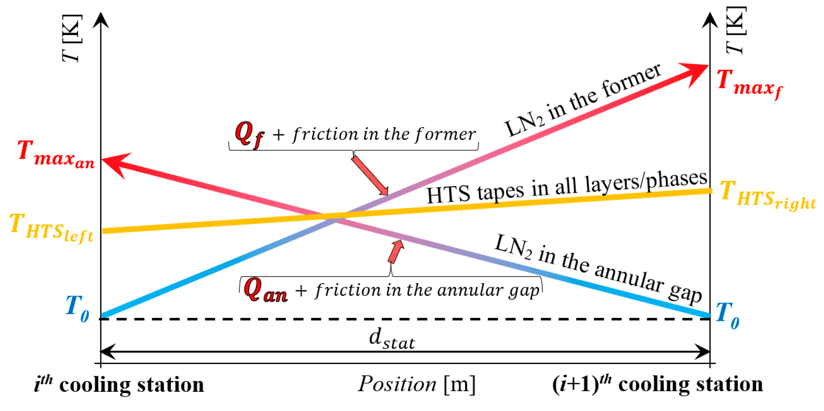
3.1. Thermo-Hydraulic Model

To effectively model a complex system like a superconducting cable within a versatile tool, several simplifying assumptions must be imposed. Particularly relevant are those related to the thermal model of the coolant flows and the cable layers. As anticipated in the previous paragraph, and as will be more evident later in this document when the dependencies of some techno-economic parameters on the cable temperatures will be explained, the fluid dynamic conditions of the fluids, along with the temperature of the HTS tapes, significantly influence the cable system’s design. Assuming modularity in the cable structure implies that the coolants absorb the same amount of heat within their respective ducts across each cable segment, named $Q_f$ and $Q_{an}$ for the LN₂ flows in the former and annular gaps, respectively, as depicted in Figure 2. Additionally, these thermal inputs are approximated to be uniformly absorbed along the length of a segment. This assumption, combined with the effect on the temperature and pressure due to friction with the ducts’ walls (also assumed to be uniform along the cable length), allows considering the linear temperature increases and linear pressure drops of the fluids from their initial fluid dynamic conditions.

Figure 3 illustrates the temperature trends of the two counterflows of LN₂ within a generic cable segment. As assumed in this study, both flows exit each intermediate or termination cooling station under identical initial temperature and pressure conditions, named $T_0$ and $P_0$, respectively. The directions of the flows and the proportion between their maximum temperatures depicted in the figure are arbitrary.

It is worth noting that the heat source $Q_{cl}$ is not present in Figure 3, instead appearing in Figure 2. Indeed, this corresponds to the power dissipated by the current leads. It is assumed that this heat is individually managed by the termination cooling stations, where the current leads are located, using a cooling flow distinct from the one circulating through the rest of the cable.

In equation terms, the linear variations in temperature and pressure of the fluid in one of the two pipes along a cable segment of a length $d_{stat}$ $\mathsf{\Delta }T$ and $\mathsf{\Delta }P$, respectively, are calculated using the simple set of analytic equations in Equations (1)–(5), which were adapted for this model from [40]. To avoid the redundancy of writing the same equations for both fluids, the formulae for a single generic pipe having the subscript h are reported. For each fluid flow, readers can replace these subscripts with the one referring to the former or the annular gap:

$$\mathsf{\Delta }{P}_h=d_{stat}\left({\displaystyle \frac{{\rho }_{LN2} {{\nu }_{LN{2}_h}}^2 f_{LN{2}_h}}{4 R_h}}\right)+\left(g{\rho }_{LN2}\mathsf{\Delta }height\right)$$

(1)

$$\mathsf{\Delta }{T}_h=d_{stat}\left({\displaystyle \frac{ {{\nu }_{LN{2}_h}}^2 {f_{LN2}}_h}{4 R_h c{p}_{LN2}}}\right)+\left[{\displaystyle \frac{Q_h\left({T_h}_1, {T_h}_2\right)}{\dot{{2 m}_{LN2}} c{p}_{LN2}}}\right]$$

(2)

$${\nu }_{LN{2}_h}={\displaystyle \frac{\dot{m_{LN2}}}{{\rho }_{LN2} \pi {R_h}^2}}$$

(3)

$$f_{LN{2}_h}={\left\{-1.8 \mathrm{l}\mathrm{n}\left[{\left({\displaystyle \frac{{\epsilon }_h}{7.4 R_h}}\right)}^{1.11}+\left({\displaystyle \frac{6.9}{R{e}_h}}\right)\right]\right\}}^{-2}$$

(4)

$$R{e}_h={\displaystyle \frac{2 R_h {\nu }_{LN{2}_h} {\rho }_{LN{2}_h}}{{\mu }_{LN2}}}$$

(5)

where ${\rho }_{LN2}$, ${\nu }_{LN{2}_h}$, $c{p}_{LN2}$, and ${\mu }_{LN2}$ are the density, velocity, heat capacity, and dynamic viscosity of LN₂, respectively. These values would depend on the fluid temperature and pressure as well but are approximated here as constants by using their average values within the chosen operating temperature and pressure ranges (i.e., 67–77 K). Here, ${\epsilon }_h$ is the roughness of the pipe h, $g$ is gravity’s acceleration, and $\mathsf{\Delta }height$ is the height difference between the two ends of a cable segment (assumed equal for all cable segments) [41], while ${f_{LN2}}_h$ and $R{e}_h$are the friction factor and the Reynolds number of the nitrogen flowing in the pipe h. The expression in Equation (4) is computed by approximating the implicit Colebrook–White equation for corrugated cylindrical and centric tubes [42] and by using the explicit Haaland equation [43].

In Equation (2), the correlation between $Q_f$or $Q_{an}$ (collectively represented as $Q_h$) and the temperatures of the two fluids is made explicit to underline that each of the respective equations applied to both fluids is implicit and that their combined system must be solved in numerical form.

Figure 3 presents the temperature trend considered for all HTS layers of the cable. Specifically, it is assumed that at each conductor’s cross-section (i.e., any point along the longitudinal axis of the cable), the temperature of all superconducting tapes corresponds to the arithmetic average between the nitrogen temperatures in the two ducts enclosing the conductor. Even when accounting for radial symmetry, temperature variations might be present among the HTS layers based on their positioning relative to the two coolant flows. However, achieving a more accurate calculation would require modeling the heat transfer within the cable’s cross-section, which would make the model calculations more cumbersome. Therefore, it was avoided.

By applying this simplifying assumption, the temperature trend of the HTS layers in a generic cable segment is also linear. This simplification facilitates the calculation of the HTS temperature at the two ends of the segment (arbitrarily referred to as the left and right sides), combining the initial temperature and the results of Equation (2). Referring to Figure 3, the HTS temperature on the left side of a segment corresponds to $T_{HT{S}_{left}}=\left(T_0+T_{{max}_{an}}\right)/2$, while that on the right side is $T_{HT{S}_{right}}=\left(T_0+T_{{max}_f}\right)/2$, where $T_{{max}_{an}}$ and $T_{{max}_f}$ are computed from Equation (2) as $T_0+\mathsf{\Delta }{T}_{an}$ and $T_0+\mathsf{\Delta }{T}_f$, respectively.

3.2. Electrical Model

The geometry of the coaxial cable plays a critical role in determining the distribution of current across its layers and phases. An erroneous selection of geometric parameters may result in significant current imbalances or force the superconductor to operate under undesirable conditions. This study considers some simplifying assumptions to reliably estimate the distribution with relatively straightforward analytical formulae.

First, the HTS tapes wound on each layer are assumed to be connected in parallel and share their corresponding layer current of the module $\left|\underset{\_}{I_{i,j}}\right|$ evenly. Then, it is assumed that the cable connects a direct symmetrical three-phase generator system to a three-phase wye load, having a load factor $\mathrm{c}\mathrm{o}\mathrm{s}\phi$. In computing the current distribution, the electrical resistance of each conductive layer is neglected, under the assumption that the HTS tapes operate well below their critical current threshold. Consequently, the current in the individual layers can be determined by solving the following system:

$$\left\{\begin{array}{c}{\displaystyle \frac{V_{rms}}{\sqrt{3}}}={\displaystyle \sum _{i=1}^3}{\displaystyle \sum _{j=1}^{{nl}_i}}j\omega M_{1,k-i,j}\underset{\_}{I_{i,j}}+{\displaystyle \sum _{j=1}^{{nl}_1}}{Z}_L e^{j\phi } \underset{\_}{I_{1,j}}+\underset{\_}{V_s} for k=1,{\dots ,nl}_1 \\ \begin{array}{c} \\ {\displaystyle \frac{V_{rms}}{\sqrt{3}}}{e}^{-j{\displaystyle \frac{2}{3}}\pi }={\displaystyle \sum _{i=1}^3}{\displaystyle \sum _{j=1}^{{nl}_i}}j\omega M_{2,k-i,j}\underset{\_}{I_{i,j}}+{\displaystyle \sum _{j=1}^{{nl}_2}}{Z}_L e^{j\phi } \underset{\_}{I_{2,j}}+\underset{\_}{V_s}\end{array} for k=1,{\dots ,nl}_2 \\ \begin{array}{c}\begin{array}{c} \\ {\displaystyle \frac{V_{rms}}{\sqrt{3}}}{e}^{j{\displaystyle \frac{2}{3}}\pi }={\displaystyle \sum _{i=1}^3}{\displaystyle \sum _{j=1}^{{nl}_i}}j\omega M_{3,k-i,j}\underset{\_}{I_{i,j}}+{\displaystyle \sum _{j=1}^{{nl}_3}}{Z}_L{e}^{j\phi } \underset{\_}{I_{3,j}}+\underset{\_}{V_s} for k=1,\dots ,{nl}_3 \end{array}\\ \begin{array}{c} \\ {\displaystyle \sum _i^3}{\displaystyle \sum _j^{{nl}_i }}\underset{\_}{I_{i,j}}=0 \end{array}\end{array}\end{array}\right.$$

(6)

where $V_{rms}$ is the rms value of the phase-to-phase voltage, $\omega$ is the pulsation of the AC current with a frequency f, and $\underset{\_}{V_s }$ is the voltage of the common wye node. Note that the complex layer currents $\underset{\_}{I_{i,j}}$ are computed in Equation (6) for the maximum power $P_{max}$ for which the cable is sized. Thus, they correspond to the peak current amplitudes observed during the cable’s operation. However, in practice, the cable will also operate at lower power levels, as will be elaborated upon in Section 3.4. Nonetheless, the current distribution will consistently remain proportional. Moreover, as the tapes in each layer are in parallel, the current amplitude $\sqrt{2} \left|\underset{\_}{I_{tap{e}_{i,j}}}\right|$, which is required for applying the grading approach described in Section 2.2, is simply computed by dividing $\sqrt{2}\left|\underset{\_}{I_{i,j}}\right|$ by the corresponding number of tapes.

Then, $Z_L$ in Equation (6) is the impedance of the three-phase load, defined as

$$Z_L={\displaystyle \frac{{V_{rms}}^2}{P_{max}}}$$

(7)

As for the inductances in Equation (6), $M_{1,k-i,j}$, $M_{2,k-i,j}$, and $M_{3,k-i,j}$ are the mutual inductances between the layers of the first, second and third phases, respectively, and all of the other layers. In general terms, the mutual inductance of the jth layer of the ith phase and the kth layer of the zth phase are computed as shown in [44,45,46] for a generic cable segment:

$$M_{i,j,k,z}=d_{stat}{\displaystyle \frac{{\mu }_0}{4\pi }}\left[2\mathit{ln}\left({\displaystyle \frac{R_n}{R_{i,j}}}\right)+{\displaystyle \frac{R_{k,z}}{R_{i,j}}}\mathit{tan}\left({\alpha }_{j,k}\right)\mathit{tan}\left({\alpha }_{k,z}\right)\right]$$

(8)

where $R_{i,j}$ is the inner radius of the jth layer of the ith phase and $R_n$ is the inner radius of the copper neutral conductor, which is known once the radius of the underlying insulating layer is determined through the optimization procedure (see Section 3.5).

3.3. Magnetic Model

Compared with previous versions of OSCaR for HTS cables [36,37], a magnetic model is also included here to calculate the magnetic field applied inside and outside of the conductor. This model operates with the results of the electrical model under the assumption that the impedance rise within the individual HTS layers does not affect the current distribution. However, these magnetic effects impact the performance of the coated conductor and the cost of the land to be acquired around the cable.

Having assumed radial symmetry for the cable structure, only the radial ($B_r$) and tangential components $\left(B_t\right)$ of the magnetic field with respect to the tapes’ main face have to be computed. These expressions, reported in Equation (9), refer to the field applied at the average radius of the kth layer of the zth phase (the midpoint between them being its inner and outer radii, called ${R_{mean}}_{k,z}$). Thus, this accounts for the current flowing across all layers. The analytic equations are derived while assuming each HTS layer is a cylinder with an inner radius $R_{i,j}$ and outer radius $R_{i,j}+t_{HTS}$, where a current $\underset{\_}{I_{i,j}}$ which is uniformly distributed across the surface flows [47]:

$$\left\{\begin{array}{c}{B}_{r_{k,z}}={\displaystyle \sum _{i=1}^3}{\displaystyle \sum _{j=1}^{{nl}_i}}{\mu }_0\left(\left(R_{i,j}+t_{HTS}\right)-{R_{mean}}_{k,z}\right){\displaystyle \frac{\left|\underset{\_}{I_{i,j}}\right| sin\left({\alpha }_{i,j}\right)}{\pi \left[{\left(R_{i,j}+t_{HTS}\right)}^2-{R_{i,j}}^2\right]}}\\ B_{t_{k,z}}={\displaystyle \sum _{i=1}^3}{\displaystyle \sum _{j=1}^{{nl}_i}}{\mu }_0{\displaystyle \frac{\left[{{R_{mean}}_{k,z}}^2-{R_{i,j}}^2\right]}{2 R_{k,z}}}{\displaystyle \frac{\left|\underset{\_}{I_{i,j}}\right| cos\left({\alpha }_{i,j}\right)}{\pi \left[{\left(R_{i,j}+t_{HTS}\right)}^2-{R_{i,j}}^2\right]}} \end{array}\right.$$

(9)

In Equation (9), ${\mu }_0$ is the vacuum permeability, while the magnitude and the orientation of the field ($\theta$ angle), required in the $I_c\left(T_{HTS}, \left|B\right|, \theta \right)$ function, are calculated as follows:

$$\left|B_{k,z}\right|=\sqrt{{B_{r_{k,z}}}^2+{B_{t_{k,z}}}^2}; {\theta }_{k,z}=\mathrm{atan}\left({\displaystyle \frac{B_{r_{k,z}}}{B_{t_{k,z}}}}\right)$$

(10)

It is worth noting that the radial component of the magnetic field is minimal everywhere, given the arrangement of the HTS tapes on the concentric layers. However, given the significant dependence of the tape’s critical current on the radial component, the authors opted not to neglect it.

3.4. Time-Varying Power Transferred by the Line

The choice of a cable’s rated power is crucial in defining its resulting design. This work focuses on HVAC cables capable of transferring extremely high-power loads. Some of the values proposed in this study may be considered speculative, given the current lack of network infrastructure to accommodate lines with power values exceeding 1–2 GW. Nonetheless, these high-power lines could potentially be required in the future, especially if their techno-economic viability is demonstrated, considering the growing scale of single-site power plants and the rising demand for localized energy-intensive loads [48,49,50].

Furthermore, it is important to note that a cable may not operate at its full capacity throughout its whole expected lifespan. Power curves for the following hours, months, and years can be hypothesized to depict fluctuating power demands over time and the specifics of a network. Figure 4 shows the time-varying power trend adopted in this study for any optimized superconducting line (in blue) over the course of one year. The power values are normalized, allowing for the curve to be scaled by the selected peak power. Notably, the curve does not reflect the actual progression of power from the beginning to the end of the year, as in reality, power fluctuates on a daily basis. In Figure 4, the time durations throughout the year during which a specific power level is applied are aggregated, and these power levels are then arranged conveniently in descending order. It is considered that the same power curve can be applied identically for all years of the lifespan expected for the designed line.

In the optimization tool, the maximum power during the year is taken as a benchmark. This is used, for example, to calculate the amount of superconducting tape needed, the maximum instantaneous losses, and the corresponding temperature increase in the coolant flows. However, for an accurate computation of the energy dissipation over the line’s lifespan—upon which the operating costs of the cooling system depend (as will be detailed in Section 4.6)—the actual power curve should be used. Nonetheless, this approach would substantially increase the computation time within the optimization algorithm proposed. Indeed, this would require repeating the numerical calculations to determine the thermal inputs, temperatures, and operating costs for every individual of a single generation of the genetic algorithm and for all the time intervals discretized from the curve in Figure 4. Moreover, this time-consuming numerical resolution must then be iterated at each step from one generation of the genetic algorithm to the next one until the convergence criteria are met.

Hence, it is deemed practical to optimize a cable by calculating the cost function as if the cable were transferring its maximum power throughout the year. This scenario is represented by the dashed black curve in Figure 4. This enables performing the necessary numerical computation only once for each individual in a generation of the genetic algorithm, thereby significantly reducing the calculation times. However, this approach tends to overestimate the total losses and the corresponding operating costs over the life of the cable. The area highlighted in yellow in Figure 4 represents the overestimation of the cable’s energy consumption assumed during the optimization process, following the use of the dotted horizontal line compared with the more realistic power curve. To mitigate this approximation, once the optimal system parameters and the corresponding cable design are determined while assuming a constant peak power, only the operating costs are re-calculated, considering the real power curve. This recalibration process is executed just once when the optimization procedure is concluded, thereby maintaining the computational efficiency of the algorithm.

3.5. Calculation of the Thicknesses of the Dielectric Layers

Once the optimized variables of the system are derived, the whole cable geometry can be determined. This corresponds to the inner and outer radii of each layer composing the coaxial design of the cable. This process is performed sequentially from the innermost layer’s radius, which corresponds to the inner radius of the former $R_f$, and requires knowing the thicknesses of the various layers, as detailed in Section 2.1. These thicknesses are set by the user for all layers (numerical examples will be given in Section 7.2), except for those referring to the insulating layers.

After determining the outer radii of the superconducting layers directly beneath each of the three insulating layers in the cable (hereinafter generalized as the mth insulating layer), these values also correspond to the inner radius of the mth layer $R_{in{t}_{ins m}}$. As for their thicknesses, these have to be sized to withstand two distinct electrical stress conditions which might occur during cable operations: the AC nominal voltage and the lightning impulse voltage [51,52,53]. For each scenario, a corresponding insulation thickness is required:

$${t_{in{s}_{AC}}}_m=R_{in{t}_{ins m}}\left[exp\left({\displaystyle \frac{k_{1_{AC} }{k}_{2_{AC}} k_{3_{AC}}{ V}_{AC}}{R_{in{t}_{ins m}} E_{AC}}}\right)-1\right]$$

(11)

$${t_{in{s}_{im}}}_m=R_{in{t}_{ins m}}\left[exp\left({\displaystyle \frac{k_{1_{im} }{k}_{2_{im}} k_{3_{im}}{ V}_{im}}{R_{in{t}_{ins m}} E_{im}}}\right)-1\right]$$

(12)

where $k_{1_{AC}}$ and $k_{1_{im}}$ are the corrective aging coefficients which compensate for the degradation of the dielectric properties under electric stress. $k_{2_{AC}}$ and $k_{2_{im}}$ are the corrective temperature coefficients taken into account when considering potential insulation failures due to heat aging. $k_{3_{AC}}$ and $k_{3_{im}}$ are the correction safety coefficients, which can be used as design safety margins. $V_{im}$ is the lightning impulse target’s withstanding voltage, and $V_{AC}$ is the AC rated voltage, usually calculated as $2.5\left(\sqrt{2}{V}_{rms}\right)/\sqrt{3}$ according to IEC 62067 [51,54]. $E_{AC}$ and $E_{im}$ are the breakdown voltages for both scenarios. These parameters depend on the insulating material selected and can be found in the literature.

Then, to comply with both scenarios, the thickness of the mth insulating layer is taken to be equal to the maximum value calculated in the two conditions, or

$${t_{ins}}_m=max\left({t_{in{s}_{AC}}}_m, {t_{in{s}_{im}}}_m\right)$$

(13)

4. Cost Function to Be Minimized

As outlined in Section 2, the optimization tool identifies the combination of system variables which minimizes the total cost of the cable system $C_{tot}$. Therefore, it is relevant to have a comprehensive cost function which can be applied consistently to different cable designs, whether superconducting or conventional. The objective function proposed in this study is reported here, whose indexes correlate to the system variables and, consequently, to the resultant cable design. The authors tried to make this function as comprehensive as possible, but users can possibly modify or expand it depending on their specific requirements:

$$\begin{gathered} C_{tot}={C_{HTS}}^{\%}+{C_{ins}}^{\%}+{C_{LN2}}^{\%}+C_{Cu}+{C_{coo{l}_{cap}}}^{\%}+C_{coo{l}_{op}}+{C_{cryostat}}^{\%}+C_{vac}+ \\ +C_{cl}+C_{land}+{C_{cab}}^{\%}+C_{man}+C_{dis}+C_{comm}+C_{install}+C_{other} \end{gathered}$$

(14)

where ${C_{HTS}}^{\%}$, ${C_{ins}}^{\%}$, ${C_{LN2}}^{\%}$, and $C_{Cu}$ are the costs of the superconducting material, the electrical insulation, the liquid nitrogen, and the copper required for the neutral conductor layer, respectively, ${C_{coo{l}_{cap}}}^{\%}$ and $C_{coo{l}_{op}}$ are the capital and operating costs for the cooling stations, respectively, ${C_{cryostat}}^{\%}$, $C_{vac}$, and $C_{ter}$ are the costs of the cryostat, the vacuum pump system, and the cable current leads, respectively, $C_{land}$ is the cost of purchasing the land to install the cable, ${C_{cab}}^{\%}$, $C_{man}$, and $C_{dis}$ are the cabling, maintenance, and dismantling costs, respectively, and $C_{comm}$, $C_{install}$, and $C_{other}$ represent the costs related to a cable project’s commissioning and management, the civil engineering activities required for on-site installation, and the other costs which cannot be categorized in the previous indexes, respectively.

Hereafter, the cost indexes expressed with uppercase letters (C) will indicate the total cost, while lower case letters (c) will be used to represent their unitary cost.

4.1. Approach for the Quantitative Discounting of Selected Cost Indexes

Readers may observe that certain terms in Equation (14) are denoted with the superscript %. This graphic notation distinguishes the capital costs for which the authors have decided to apply quantitative discounting. Indeed, it is reasonable to assume that by purchasing large quantities of certain materials or components, as might occur when designing long lines, the producer or investor can benefit from an appropriately discounted unit price compared with that when purchasing smaller quantities.

Listed here are the logical steps for calculating this quantitative discount for each of the cost indexes marked with the superscript % in Equation (14):

(1)

A reference quantity (called $q_{re{f}_x}$, where the subscript x can be replaced with the corresponding cost term) is set for each discounted index, whether it be a length, a weight, a volume, or the number of components. These quantities correspond to the reference case for which the authors have assumed fixed unit costs ($c_x$), such as the materials required for a 50 km HTS cable. By carrying out parametric analyses with the proposed tool, different case studies from the reference one can be investigated, resulting in different optimized designs and material or component quantities.

If these quantities are greater than their reference values, then a reduction in the unit cost is expected. Conversely, if the optimized quantities fall below their reference values, then it is reasonable that the buyer will have to pay a higher unit price.

(2)

A multiplicative coefficient relative to the reference quantity is set (referred to as $m_{{\%}_x}$), corresponding to a discount of the unit cost, called $d_{{\%}_x}$. To give a quantitative example, supposing $q_{re{f}_x}$ is equal to 100 km, $m_{{\%}_x}$ is equal to 5, and $d_{{\%}_x}$ is equal to 20%, if the optimized cable design requires purchasing a quantity of the material or component x equal to $q_{re{f}_x}· m_{{\%}_x}$= 500 km, then the corresponding unit cost of that material or component will be lowered by 20% compared with the one set for the reference quantity. The parameter $m_{{\%}_x}$ is also used as a divisor of the reference quantity, resulting in an increase in the unit cost when the optimized quantity is lower than the reference one, corresponding again to $d_{{\%}_x}$.

(3)

It is assumed that the discount of the unit cost is linearly proportional to the optimized quantity. This discounting process is applied within maximum and minimum discounting rates compared with the reference unit cost. This corresponds to assuming that the buyer’s or manufacturer’s leverage on the unit price is limited to a certain range. For simplicity, both thresholds are set equal to $d_{{max\%}_x}$, which might then be positive or negative.

In mathematical form, the above can be summarized as

$${c_x}^{\%}=c_x\left(1-{\displaystyle \frac{ d_{{\%}_x}}{m_{{\%}_x}-1}}\right)\left({\displaystyle \frac{ q_x-q_{re{f}_x}}{q_{re{f}_x}}}\right)$$

(15)

where $c_x$ and ${c_x}^{\%}$ are the unit cost of the material or component x before and after the quantitative discounting process, respectively, and $q_x$ is the quantity of the material or component x computed during the optimization.

Figure 5 illustrates the described steps by showing the correlation between the unit price of the generic material or component x and its quantity.

In the formulae presented in the next sections which refer to the cost indexes outlined in Equation (14), the calculation for the discount of the unit cost of the corresponding material or component presented here will be omitted to avoid overcomplication. However, the unit costs will be marked with the superscript %, and in Section 7.1, examples of the $q_{re{f}_x}$, $m_{{\%}_x}$, $d_{{\%}_x}$, and $d_{{max\%}_x}$ values for the individual indexes will be provided.

4.2. Cost of the Superconducting Material

The capital cost for purchasing the HTS tapes needed for the cable is calculated as follows:

$${C_{HTS}}^{\%}={\displaystyle \sum _i^3}\left\{\left[{c_{HT{S}_i}}^{\%}\left(I_{c 77 K_i}\right)\right]{\displaystyle \sum _j^{{nl}_i}} {Tapes}_{i,j}{\displaystyle \frac{ L_{line}}{\left|cos\left({\alpha }_{i,j}\right)\right|}}\right\}$$

(16)

$${Tapes}_{i,j}=round \left({\displaystyle \frac{ 2\pi R_{i,j} \left|cos\left({\alpha }_{i,j}\right)\right|}{w_{HTS}}}\right)$$

(17)

where ${c_{HT{S}_i}}^{\%}$ is the cost per unit length of the HTS tapes of the ith phase, discounted with respect to the total length of tape acquired for that phase, and ${Tapes}_{i,j}$ is the number of HTS tapes constituting the jth HTS layer of the ith phase, having a width $w_{HTS}$.

In Equation (15), the dependency of the conductor cost per unit length on the value of $I_{c_{77 K}}$ is made explicit. This follows the approach outlined in Section 2.2. For clarity, the mathematical steps leading to the determination of $I_{c 77 K_i}$ and consequently to ${c_{HT{S}_i}}^{\%}$ are reported here as implemented within the optimization algorithm:

(1)

At each algorithm step, a specific set of system variables is examined, including the $\sqrt{2} \left|\underset{\_}{I_{tap{e}_{i,1}}}\right|/I_c\left(T_{HT{S}_{max}}, {\left|B\right|}_{i,1}, {\theta }_{i,1}\right)$ ratios.

(2)

Based on each $\sqrt{2}\left|\underset{\_}{I_{tap{e}_{i,1}}}\right|/I_c\left(T_{HT{S}_{max}},{\left|B\right|}_{i,1},{\theta }_{i,1}\right)$ ratio and the calculation of $\left|\underset{\_}{I_{tap{e}_{i,1}}}\right|$ for the innermost layer of each phase (as detailed in Section 3.2), the values of $I_c\left(T_{HT{S}_{max}},{\left|B\right|}_{i,1},{\theta }_{i,1}\right)$ are derived. These correspond to the lowest critical current values for the tapes belonging to the innermost layer of each phase occurring in a cable segment.

(3)

From the results of the thermal model (Section 3.1) and the magnetic model (Section 3.3), the higher temperature and magnetic field values within a cable segment are determined for the innermost layer of each phase. These represent the most stressful scenarios for the coated conductor in each phase, where the upper limit of the ratios between the transport currents and the critical currents are conservatively determined.

(4)

Then, the characteristic curves of the chosen coated conductor $I_c\left(T_{HTS}, \left|B\right|, \theta \right)$ are considered. These curves are generally provided by the manufacturer for a reference tape and are not always reported in dimensionless terms. These curves enable calculation of the critical current values of the reference tape under the same temperature and magnetic field conditions identified in the previous step, with one for each phase, called $I_{{c_{ref}}_{T_{HT{S}_{max}}, {\left|B\right|}_{i,1}, {\theta }_{i,1}}}$.

(5)

Similarly, using the manufacturer’s characteristic curves, the critical current value of the reference tape at 77 K and self-field is known, called $I_{{c_{ref}}_{77 K}}$.

(6)

It is assumed that the same characteristic curves valid to the reference tape can be scaled for the actual tape adopted in each phase of the optimized structure. By solving a simple proportion for each phase, the corresponding values of $I_{c 77 K_i}$ can be obtained:

$$I_{c 77 K_i}=I_c\left(T_{HT{S}_{max}}, {\left|B\right|}_{i,1}, {\theta }_{i,1}\right){\displaystyle \frac{ I_{{c_{ref}}_{77 K}}}{I_{{c_{ref}}_{T_{HT{S}_{max}}, {\left|B\right|}_{i,1}, {\theta }_{i,1}}}}}$$

(18)

(7)

Then, the $c_{HT{S}_i}$ values (before quantitative discounting) are computed by multiplying the $I_{c 77 K_i}$ values for the cost per unit length and per kiloampere of current carried by the tape at 77 K and the self-field tape (${c_{HTS}}^{kA}$), for which statistical data can be gathered from the literature:

$$c_{HT{S}_i}\left[{\displaystyle \frac{€}{m}}\right]={c_{HTS}}^{kA}\left[{\displaystyle \frac{€}{kA·m}}\right]·I_{c 77 K_i}\left[kA\right]$$

(19)

(8)

Finally, the ${c_{HT{S}_i}}^{\%}$ values are calculated by applying the quantitative discounting approach described in Section 4.1 to $c_{HT{S}_i}$.

Lastly, it is worth noting that by applying Equation (17), the condition for which the gap between adjacent tapes on the same layer should not exceed 3% of the tape width ($w_{HTS}$) to minimize the transverse component of the magnetic field applied on each tape and the resulting magnetization losses, as suggested in [34], is automatically satisfied. Indeed, Equation (17) ensures that each superconducting layer always accommodates the maximum number of tapes which can be geometrically placed side by side on the corresponding circumference and with the selected winding angle. The function $round$ in Equation (17) approximates the result to the nearest integer.

4.3. Cost of the Insulating Material

The capital cost for the insulating material is computed as follows:

$${C_{ins}}^{\%}={c_{ins}}^{\%} {\rho }_{ins} L_{line }\pi {\displaystyle \sum _m^3}\left({R_{ex{t}_{ins m}}}^2-{R_{in{t}_{ins m}}}^2\right)$$

(20)

where ${c_{ins}}^{\%}$is the insulation cost per unit weight, discounted with respect to the total weight purchased, ${\rho }_{ins}$ is the insulation mass density, and $R_{ex{t}_{ins m}}$ is the outer radius of the mth insulating layer, calculated from its inner radius $R_{in{t}_{ins m}}$ and the result of Equation (13).

4.4. Cost of the Cryogenic Fluid

The capital cost for the cryogenic fluid flowing in a closed loop within the cable in both the former and the annular gaps corresponds to

$${C_{LN2}}^{\%}={c_{LN2}}^{\%} L_{line} \pi \left[{R_{ex{t}_{an}}}^2-{R_{in{t}_{an}}}^2+{\left(R_f-t_f\right)}^2\right]$$

(21)

where ${c_{LN2}}^{\%}$ is the cost of the liquid nitrogen per unit volume, discounted with respect to the volume of coolant purchased, and $R_{ex{t}_{an}}$ and $R_{in{t}_{an}}$ are the outer and inner radii of the annular gap, respectively. $R_{in{t}_{an}}$ is derived from the inner radius ($R_n$) and the thickness ($t_n$) of the underlying copper neutral layer, while $R_{ex{t}_{an}}$ depends on $R_{in{t}_{an}}$ and the thickness $t_{an}$.

4.5. Cost of the Copper for the Neutral Conductor

The capital cost for the copper required for the neutral conductor layer is calculated as follows:

$$C_{Cu}=c_{Cu} {\rho }_{Cu} L_{line} \pi \left[{R_{ex{t}_n}}^2-{R_{in{t}_n}}^2\right]$$

(22)

where $c_{Cu}$is the copper cost per unit of weight, ${\rho }_{Cu}$ is the copper density, $R_{in{t}_n}$ is the inner radius of the copper neutral layer, corresponding to the outer radius of the third insulating layer, and $R_{ex{t}_n}$ is the outer radius of the copper neutral layer, computed as $R_{in{t}_n}+t_n$.

In the computation of the overall system costs, only the copper required for the neutral conductor was considered among the conventional materials which constituted the conductor. This index was not present in the previous published versions of OSCaR. Users can modify Equation (14) to include other components neglected here.

4.6. Capital and Operating Costs for the Cooling Stations

The operating and capital costs for cooling stations are conveniently distinguished in Equation (14) to simplify their exposition in this section. Regarding the capital costs for purchasing all the cooling stations required for the whole cable length (whose total number corresponds to $n_{stat}+2$), these are equal to

$${C_{coo{l}_{cap}}}^{\%}={\displaystyle \sum _k^{n_{stat}+2}}{C}_{{cool}_{fixed}}+\left[\left({c_{cryocooler}}^{\%} Q_{c_k} \right){\beta }_Q\right] {\beta }_r$$

(23)

$$Q_{c_k}=\left\{\begin{array}{c}{Q}_f+Q_{an} if k=intermediate station \\ Q_{an}+Q_{cl} if k=left termination station \\ Q_f+Q_{cl} if k=right termation station \end{array}\right.$$

(24)

where ${c_{cryocooler}}^{\%}$ is the cost of each cryocooler system per unit of cooling power to extract ($Q_k$), which is discounted following the approach described in Section 4.1 according to the total number of cooling stations, ${\beta }_Q$ serves as a markup factor to accommodate potential heat peaks and address the practical difficulty of finding cooling devices precisely matching the required sizes in the market (in these cases, the superior size is selected), ${\beta }_r$ is a markup factor applied to consider the cost of those cooling station components for which no parametric function has been identified (circulation pumps, LN₂ tank, and accessory components), assumed to correspond to a certain percentage of the cryocooler cost, $C_{{cool}_{fixed}}$ accounts for the fixed costs required for each cooling station aside from the device cost, such as installation, maintenance, and disposal, and $Q_{c_k}$ is the sum of the heat contributions which must be removed by the kth cooling station from the LN₂ inlet flows it has to handle. A detailed explanation of the terms $Q_f$, $Q_{an}$, and $Q_{cl}$ will be provided in Section 5.

From Equation (24), it can be understood that the only differentiation between the capital costs of the various cooling stations concerns the intermediate and termination ones, with the latter being distinguished further between the two cable sides (left and right), as these are designed to manage different nitrogen flows or additional heat inputs, such as $Q_{cl}$.

Moreover, it is important to highlight that the cooling system considered in this study is not designed with redundancy. Nonetheless, an additional markup factor could be included in Equation (23) to accommodate this potential design choice.

Concerning the costs to operate all the cooling stations, these correspond to

$$C_{coo{l}_{op}}={\displaystyle \sum _k^{n_{stat}+2}}\left\{{\displaystyle \sum _z^{yr}}{c}_{kWh}{h}_y\left[\left({\displaystyle \frac{ Q_{c_k}}{{\eta }_{cry}}}{\displaystyle \frac{\left(T_a-T_0\right) }{ T_0}}\right)+{\displaystyle \frac{ Q_{p_k}}{{\eta }_p}}\right]{\displaystyle \frac{ 1}{{(1+\psi )}^z}}\right\}$$

(25)

$$Q_{p_k}=\left\{\begin{array}{c}\dot{m_{LN2} }{\displaystyle \frac{ \mathsf{\Delta }{P}_f+\mathsf{\Delta }{P}_{an}}{{\rho }_{LN2}}} if k=intermediate station \\ {\displaystyle \frac{ \dot{m_{LN2} }\mathsf{\Delta }{P}_{an}}{{\rho }_{LN2}}} if k=left termination station\\ {\displaystyle \frac{ \dot{m_{LN2} }\mathsf{\Delta }{P}_f}{{\rho }_{LN2}}} if k=right termation station \end{array} \right.$$

(26)

where $yr$ represents the expected years of service for the cable system, $h_y$ is the annual operational hours, $c_{kWh}$ is the actual energy cost for non-residential consumers in the region where the cable is planned to be installed, $Q_{c_k}$ is computed from Equation (24), (In Equation (25), the temperature ratio involving the LN₂ inlet temperature $T_0$ and the average ambient temperature during the year at the cable installation site $T_a$ corresponds to the inverse Carnot efficiency.) and $Q_{p_k}$ stands for the hydraulic power supplied by the circulation pumps to the liquid nitrogen flows to restore their initial pressure $P_{0 }$ after their corresponding drops, computed with Equation (1). In Equation (26), $\mathsf{\Delta }{P}_f$ and $\mathsf{\Delta }{P}_{an}$ are the pressure drops in the nitrogen flowing in the former and in the annular gap, respectively. It is worth noting that the termination stations have to handle a single pressure drop, as they must restore the pressure in a single inlet flow. Then, ${\eta }_{cry}$ is the efficiency of the cooling system, and ${\eta }_p$ is the efficiency of the circulation pumps. Finally, $\psi$ is the annual effective discount rate for the operating costs, which varies based on the country of cable installation. In this approach, the impact of price inflation has been neglected.

It should be kept in mind that, as detailed in Section 3.4, the cable design is optimized by minimizing Equation (14) with the simplifying hypothesis of having a constant $P_{max}$ over all the yearly timespans ($h_y$) and consequently assuming a constant $Q_{c_k}$ and $Q_{p_k}$. Upon completing the optimization process, $C_{coo{l}_{op}}$ is recalculated, summing the operating costs computed with Equation (25) for the single time intervals during a year where the delivered cable power and the corresponding $Q_{c_k}$ and $Q_{p_k}$ values vary. This approach operates under the assumption that it is reasonable to adjust the power output of the cooling and pumping stations, originally sized for a maximum rated power, based on the instantaneous power requirements.

4.7. Cost for the Land to Be Purchased to Install the Cable

Compared with the previous references to OSCaR [35,36,37], the capital cost for purchasing the land required to install a superconducting cable in its tunnel and the land around it, corresponding to the buffer zone, to comply with the law’s tolerable magnetic field limits is added in Equation (14). It is computed as follows:

$$C_{land}=c_{land} L_{line} 2 ·max\left(R_{{field}_{max}},R_{install}\right)$$

(27)

where $c_{land}$is the cost per unit surface for the land at the installation site. For long lines crossing differently urbanized and costly areas, an average cost or a more discretized calculation approach should be considered.

$R_{{field}_{max}}$ is the farthest radial location from the central axis at which a magnetic field produced by the cable and exceeding the permitted field level persists. For three-phase AC concentric geometries, the magnetic field practically cancels out beyond the conductor, even though the currents in the three phases are not perfectly balanced. Even if a strict magnetic field threshold is adopted to evaluate the buffer zone (i.e., 3 μT), $R_{{field}_{max}}$ nearly corresponds to the cable’s outer radius. In such scenarios, the radial distance necessary for tunnel excavation and cable installation ($R_{install}$) is used to calculate the required land to be purchased in Equation (27). However, for cables with different designs, whether superconducting or not, $R_{{field}_{max}}$ might be greater than $R_{install}$, and thus the first should be employed in Equation (27). $R_{{field}_{max}}$ can be computed by checking the magnetic field at increasing radial distances from the conductor, such as by replacing the term ${R_{mean}}_{k,z}$ in Equation (9).

The authors considered it relevant to include this index in the cost analysis to ensure a fairer comparison with other cable technologies. Indeed, one potential economic (and social) benefit of coaxial superconducting lines may be their reduced land usage to comply with magnetic field constraints, in comparison, for instance, with the large land footprint required for conventional overhead or underground high-power lines.

4.8. Other Cost Indexes

Lastly, the remaining terms in Equation (14), namely ${C_{cryostat}}^{\mathrm{\%}},{C_{vac},C}_{cab}$, $C_{man}$,$C_{dis}$, and $C_{other}$ are computed by multiplying the corresponding values per unit cable length, which are ${c_{cryostat}}^{\mathrm{\%}},{c_{vac},c}_{cab}$, $c_{man}$,$c_{dis}$, $c_{comm}$, $c_{install}$, and $c_{other}$, respectively, by $L_{line}$. It is worth noting that ${c_{cryo}}^{\mathrm{\%}}$ is discounted with respect to the length of the cryostat to purchase, which is equal to $L_{line}$.

Regarding $C_{ter}$, it is taken as a fixed value not requiring further multiplicative factors and which takes into account the cost of three-phase terminations at both sides of the cable.

While ${C_{cryostat}}^{\mathrm{\%}},{C_{vac},C_{ter},C}_{cab}$, $C_{comm}$, $C_{install}$, and $C_{other}$ are capital costs, $C_{man}$ and $C_{dis}$ are operating costs which have to be discounted in a similar manner to that performed in Equation (25). In practice, this is carried out as follows:

$$C_{man}={\displaystyle \sum _z^{yr}} {\displaystyle \frac{{L_{line} c}_{man}}{yr {(1+\psi )}^z}}$$

(28)

$$C_{dis}={\displaystyle \frac{{L_{line} c}_{dis}}{ {(1+\psi )}^{yr}}}$$

(29)

where $C_{dis}$ is discounted, supposing this cost component is paid directly at the end of the cable’s life.

5. Calculation of the Loss Contributions

An adequately precise estimation of the losses and the heat inputs during cable operation is crucial for accurately sizing the refrigeration system and the corresponding capital and operation costs. Moreover, losses directly impact the temperatures of the cryogenic fluid and the HTS tapes, consequently affecting all parameters of the cable’s design.

As described in Section 3.1, the nitrogen flows within the former and the annular gap share the heat inputs in each cable segment. The cooling stations deal with these losses consistently with the LN₂ flows they manage, with the termination ones also handling the heat generated by the current leads, as explained in Equation (24) using the arbitrary reference scheme from Figure 2.

Although adopting finite element methods (FEMs) for computing the thermal inputs in a complex cable structure could lead to quite accurate outcomes, this would demand considerable computational times, especially within a genetic optimization algorithm which recursively evaluates a great number of potential results at each step. Hence, in this context, the preference is for widely accepted analytical formulae, which offer faster computational solutions. The following equation describes the calculation of $Q_f$ and $Q_{an}$ over a cable segment of a length $d_{stat}$, as performed with the tool:

$$\left\{\begin{array}{c}{Q}_f\left(T_{{max}_f},T_{{max}_{an}}\right)={\displaystyle \frac{Q_{AC}\left(T_{{max}_f},T_{{max}_{an}}\right)+Q_{ins}+Q_{ed}}{2}} \\ Q_{an}(T_{{max}_f},T_{{max}_{an}})=Q_{cryo}\left(T_{{max}_{an}}\right)+{\displaystyle \frac{Q_{AC}\left(T_{{max}_f},T_{{max}_{an}}\right)+Q_{ins}+Q_{ed}}{2}}\end{array}\right.$$

(30)

where $Q_{AC}$ represents the AC losses produced in the HTS tapes, $Q_{ins}$ represents the losses generated in the dielectric layers, $Q_{ed}$ is the eddy current losses in the normal conducting materials, and $Q_{cryo}$ is the heat input from the cryostat walls. Equation (30) further details the correlation between $Q_f$ or $Q_{an}$ with the temperatures of the two fluids, which was already explicated in Equation (2).

Furthermore, it is assumed that the losses generated in the conductor, $Q_{AC}$, $Q_{ins}$, and $Q_{ed}$ are equally shared between the two fluids in contact. On the contrary, the thermal inputs coming from the cryostat are assumed to be absorbed only by the nitrogen flowing in the annular gap, given its proximity to the cable’s exterior. Further analysis of the heat distribution along a cable cross-section could lead to different repartitions of the heat contributions between the two fluids.

Regarding the losses generated in the current leads at the terminations ($Q_{cl}$), these are computed by multiplying the rated maximum current per phase by a parameter $q_{cl}$, corresponding to the losses per unit of current. This term is then multiplied by the required number of current leads, which in the case of an AC coaxial cable corresponds to three current leads per cable side [20].

The next sections will detail the single loss contributions reported in Equation (30).

5.1. AC Losses Generated in the HTS Tapes

With the purpose of adopting a simple analytical approach for discussion, the well-known Norris’s formula for thin strips is implemented in the proposed tool to compute the AC losses produced in the HTS tapes of the cable [55]. Each tape is approximated as a straight independent conductor having a uniform current distribution over a rectangular cross-section. This can be considered a precautionary choice since, generally, Norris’s model provides an upper limit to the estimated AC losses compared with other approaches [38,56,57].

As shown in Figure 3, it is assumed that the HTS tapes’ temperature varies linearly along the longitudinal coordinate of a cable segment x, while the magnetic field distribution in the cross-section can be considered constant. $T_{HTS}$ is bounded between $T_{{max}_f}$ and $T_{{max}_{an}}$, and for this reason, the function $Q_{AC}\left(T_{{max}_f},T_{{max}_{an}}\right)$ has been made explicit in Equation (30). This temperature variation produces a corresponding trend of the tapes’ critical current over a segment. As the AC losses strictly depend on $I_c$, this should be taken into account in the computation. For this reason, the calculation of $Q_{AC}$ is discretized over some portions of the tape length, corresponding to the sub-segments where the function $I_c\left(T_{HTS}\left(x\right), {\left|B\right|}_{i,j}, {\theta }_{i,j}\right)$ is applied and considered constant. This procedure has to be implemented for each HTS layer of the cable, as each of them might carry a different current and have a slightly different applied magnetic field. Thus, Equation (31) presents an integral over the HTS tape length of each layer in a cable segment ${L_{lay}}_{i,j}$:

$$Q_{AC}={\displaystyle \sum _i^3}{\displaystyle \sum _j^{{nl}_i}}{\displaystyle \underset{0}{\overset{{L_{lay}}_{i,j}}{\int }}}\left\{{\displaystyle \frac{{\mu }_0 f}{\pi }}{\left[I_c\left(T_{HTS}\left(x\right), {\left|B\right|}_{i,j}, {\theta }_{i,j}\right)\right]}^2 {\xi }_{i,j}(x)dx\right\}$$

(31)

$${L_{lay}}_{i,j}={Tapes}_{i,j}{\displaystyle \frac{d_{stat} }{ \left|cos\left({\alpha }_{i,j}\right)\right|}}$$

(32)

$${\xi }_{i,j}\left(x\right)=\left(1-F_{i,j}\left(x\right)\right)\ln \left(1-F_{i,j}\left(x\right)\right)+\left(1+F_{i,j}\left(x\right)\right)\ln \left(1+F_{i,j}\left(x\right)\right)F_{i,j}^2\left(x\right)$$

(33)

$$F_{i,j}(x)={\displaystyle \frac{\sqrt{2} \left|\underset{\_}{I_{i,j}}\right| }{{Tapes}_{i,j}· I_c\left(T_{HTS}\left(x\right), {\left|B\right|}_{i,j}, {\theta }_{i,j}\right)}}$$

(34)

where $F_{i,j}$ is the ratio between the amplitude of the operating current and the critical current of the jth layer of the ith phase. As $T_{HTS}$ varies along the coordinate x, so do $I_c$ and $F_{i,j}$ in Equation (34). As described in Section 2.2, for all the tapes of the layers belonging to the ith phase, the term $F_{i,j}$ does not exceed the corresponding optimized value $\sqrt{2}\left|\underset{\_}{I_{tap{e}_{i,1}}}\right|/I_c\left(T_{HT{S}_{max}}, {\left|B\right|}_{i,1}, {\theta }_{i,1}\right)$.

5.2. Losses Generated in the Insulating Layers

The dielectric losses produced in the three insulating layers of the cable are computed as follows [41]:

$$Q_{ins}={\displaystyle \sum _w^3}\left({2 \pi f d}_{stat} {tan\delta }_{ins} Capa{citance}_m V_{rms}^2\right)$$

(35)

$$Capa{citance}_m=2 \pi {\epsilon }_{ins} {\epsilon }_0\ln \left({\displaystyle \frac{R_{ex{t}_{ins m}}}{R_{in{t}_{ins m}}}}\right)$$

(36)

where ${tan\delta }_{ins}$ and ${\epsilon }_{ins}$ are the loss tangent and permittivity of the selected dielectric, respectively, ${\epsilon }_0$ is the vacuum permittivity, and $Capa{citance}_w$ is the capacitance of the mth insulating layer of a cable having inner and outer radii $R_{in{t}_{ins m}}$ and $R_{ex{t}_{ins m}}$, respectively, calculated as shown in Section 4.3. In this study, Tyvek PE was adopted as the insulating material instead of the more commonly utilized laminated polypropylene paper (PPLP), as the dielectric losses of PPLP are higher [58], and these might play a significant role in an HVAC cable.

5.3. Losses Due to Eddy Currents

The heat produced by the normal conducting materials present in the cable due to eddy currents are computed by multiplying the term $q_{ed}$, corresponding to the eddy current losses per unit of cable length and per unit of current, by $L_{line}$ and by the phase current [20]. This loss contribution is typically lower than the others.

5.4. Heat Entering the Cable Cryostat from the Outside

The heat load entering the cryostat from the outside in a cable segment is calculated as shown in [59] for a flexible cryostat. Users should consider whether to opt for rigid or flexible cryostats in their design, as the latter may result in thermal inputs 70% higher than those of the former [41], albeit while providing significantly more mechanical flexibility to the cable:

$$Q_{cryo}=d_{stat}{\displaystyle \frac{2\pi \lambda \left[T_{amb}-\left(T_{{max}_{an}}+T_0\right)/2\right] }{\mathrm{l}\mathrm{n}\left(R_{cry{o}_{ext}}/R_{cry{o}_{int}}\right)}}$$

(37)

where $\lambda$ is the “effective” thermal conductivity of the cryostat, equivalent to that for Multi Layer Insulation (MLI). A value of $\lambda$ equal to 0.4 mW/m∙K is set in this work based on the reported ranges [60,61,62,63]. $T_{amb}$ is the average ambient temperature at the cable installation site over a year. $R_{cry{o}_{ext}}$ and $R_{cry{o}_{int}}$ are the outer and inner radii of the cryostat, respectively. $R_{cry{o}_{int}}$ is equal to $R_{ex{t}_{an}}$, whose calculation has been described in Section 4.4, while $R_{cry{o}_{ext}}$ depends on $R_{cry{o}_{int}}$ and the thickness of the cryostat walls ($t_{cryo}$), imposed by the user.

6. Constraints Applied to the Optimization Algorithm

OSCaR identifies the optimal set of system variables outlined in Section 2.2 which minimizes the superconducting line cost function detailed in Equation (14) while complying with a set of constraints chosen by the user, which are described here. Sets of system variables not complying with one or more constraints are discarded by the optimizer.

First, each system variable can be bounded within upper and lower limits to restrict the investigation to scenarios considered plausible. Specific values for a case study will be detailed in Section 7. Subsequently, the native MATLAB function ga allows one to impose specific system variables to be integers (i.e., ${nl}_i$ and $n_{stat}$) while the remaining variables are computed as rational numbers. Then, electric and fluid dynamic constraints are applied to the cable design.

6.1. Constraints on the Correlations among Phase Currents and among Layer Currents

The HTS layer currents derived from Equation (6) add up to form the corresponding phase currents. Clearly, in the case of phases composed of single layers, the layer and phase currents are equal. For the line to be operated in real AC grids, it is imposed that the phase arrangement forms a balanced three-phase system. In the model, this is accomplished by checking that the relative difference between the rms value of each phase current compared with the designated rms phase value (${I_{phase}}_{rms})$ stays below a user-defined threshold ${{\%}_{max}}_{phases}$. In terms of equations, it is verified that

$$\left|\left|{\displaystyle \sum _{j=1}^{{nl}_i}}\underset{\_}{I_{i,j}}\right|-{I_{phase}}_{rms}\right|/{I_{phase}}_{rms}\le {{\%}_{max}}_{phases} for i=1, 2, 3$$

(38)

$${I_{phase}}_{rms}={\displaystyle \frac{P }{{\sqrt{3} V}_{rms}\mathrm{c}\mathrm{o}\mathrm{s}\phi }}$$

(39)

Similarly, a constraint is imposed to check that the superconducting layers equally share the current of the phase where they belong. This ensures a balanced workload across layers, preventing some tapes from operating at currents nearing their critical value while others remain underloaded. To achieve this, the following constraint is imposed on each layer current:

$${\displaystyle \frac{\left|\left|\underset{\_}{I_{i,j}}\right|-\left|\underset{\_}{I_{i,j+1}}\right|\right|}{max\left(\left|\underset{\_}{I_{i,j}}\right|,\left|\underset{\_}{I_{i,j+1}}\right|\right)}}\le {{\%}_{max}}_{layers} for i=1,2,3 and for j=1,\dots ,{nl}_i-1$$

(40)

where ${{\%}_{max}}_{layers}$ represents the maximum threshold set by the user for the relative difference between the amplitude of a given layer current and the amplitude of the other layer currents within the same phase.

The imposition of Equations (38) and (40) places an implicit constraint on the mutual inductances of the HTS layers and therefore on the relative winding angles and radii.

It is worth noting that in this version of OSCaR, it is no longer necessary to apply a safety criterion concerning the maximum current flowing in the HTS tapes of the optimized cable design. Indeed, this is automatically satisfied, having selected $\sqrt{2} \left|\underset{\_}{I_{tap{e}_{i,1}}}\right|/I_c\left(T_{HT{S}_{max}}, {\left|B\right|}_{i,1}, {\theta }_{i,1}\right)$ as system variables and applied corresponding safety and underload limits to these terms.

6.2. Constraints on the Maximum LN₂ Temperature Rise and Pressure Drop

As illustrated in Section 3.1, both the coolants flowing in the former and in the annular gap undergo a temperature rise and pressure drop through each cable segment due to friction with the duct walls and the heat contributions listed in Section 5. These fluid dynamic variations from the fluid’s initial conditions occur upon exiting each cooling station, set to $T_0$ and $P_0$ by the user, respectively, and corresponding to a subcooled liquid state. Carefully monitoring these variations is crucial to ensure that the nitrogen is always maintained in its liquid state and to prevent bubble formation, which could compromise the heat exchange with the HTS tape. Consequently, constraints are imposed on the maximum temperature and pressure variations from their initial conditions ${\mathsf{\Delta }{T}_{LN2}}_{max}$ and ${\mathsf{\Delta }{P}_{LN2}}_{max}$, respectively, compared with the values calculated using Equations (1) and (2):

$$\mathsf{\Delta }{T}_h\le {\mathsf{\Delta }{T}_{LN2}}_{max}$$

(41)

$$\mathsf{\Delta }{P}_h\le {\mathsf{\Delta }{P}_{LN2}}_{max}$$

(42)

These constraints have an impact on the entire cable geometry, particularly influencing the number of intermediate cooling stations required.

6.3. Constraints on the Values of $I_{c77K_i}$

The workflow described in Section 4.2 for calculating ${c_{HT{S}_i}}^{\%}$ enables the determination of the critical current values at 77 K and the self-field ($I_{c 77 K_i}$) for the HTS tapes used in each phase. Without constraints, the solver might produce impractical solutions, such as the use of extremely poor-performing (although extremely cheap) coated conductors or tapes with critical currents far exceeding current manufacturing capabilities, especially for long batches. Therefore, it is reasonable to restrict $I_{c 77 K_i}$ between realistic maximum and minimum values achievable by manufacturers $I_{c 77 K_{max}}$ and $I_{c 77 K_{min}}$, respectively, referred to here as 4 mm-wide tapes.

7. References Values Adopted for the Parametric Analyses

This section presents the references values proposed by the authors for all the user-defined parameters described throughout this article which are not optimized by the solver. These values are used to perform the parametric analyses, whose results are shown in Section 8.

7.1. References Values for the Economic Parameters

The values selected for the economic parameters described in Section 4 are displayed in

Table 1. Values of the economic parameters set in the tool.

Parameter	Unit	Value	Reference
${c_{HTS}}^{kA}$	EUR/kA∙m	100.0
$c_{ins}$	EUR M/ton	0.02	[41]
$c_{LN2}$	EUR/liter	0.16	[26]
$c_{Cu}$	EUR/kg	7.0
$c_{cryostat}$	EUR M/km	0.22	[64]
$c_{vac}$	EUR/m	52.0	[65]
$c_{cab}$	EUR M/km	2.0
$c_{man}$	EUR M/km	0.11	[41]
$c_{dis}$	EUR M/km	0.02	[41]
$c_{land}$	EUR/m2	60
$c_{comm}$	EUR M/km	0.04
$c_{install}$	EUR M/km	0.46
$c_{other}$	EUR M/km	0.28
$C_{ter}$	EUR M	0.4	[66]
$C_{{cool}_{fixed}}$	EUR M	0.5
$c_{cryocooler}$	EUR/W	25.0
${\beta }_Q$		1.1
${\beta }_r$		1.1
$c_{kWh}$	EUR/kWh	0.053
$\psi$	%	5.0

. The unit cost reported in Table 1 corresponds to the term $c_x$ in Section 4.1. The value of ${c_{HTS}}^{kA}$ (required in Equation (19)) refers to the 4 mm-wide HTS tapes, but the users can triple this value if 12 mm-wide tapes are preferred.

Then, the unit costs of certain account indexes are discounted based on their quantity as detailed in Section 4.1. The discounting process requires setting the parameters $q_{re{f}_x}$, $m_{{\%}_x}$, $d_{{\%}_x}$, and $d_{{max\%}_x}$ and applying them to compute the discounted unit costs ${c_{HTS}}^{\%}$,${c_{ins}}^{\%}$, ${c_{LN2}}^{\%}$, ${c_{cryocooler}}^{\%}$, ${c_{cryostat}}^{\%}$, and ${c_{cab}}^{\%}$. These were selected by the authors according to their sensitivity, and they are reported in

Table 2. Values used to discount some selected cost indexes.

Parameter	Unit	Value
$q_{re{f}_{HTS}}$	km	100
$m_{{\%}_{HTS}}$		5
$q_{re{f}_{insulation}}$	tons	20
$m_{{\%}_{insulation}}$		10
$q_{re{f}_{LN2}}$	liters	104
$m_{{\%}_{LN2}}$		10
$q_{re{f}_{cryostat}}$	km	20
$m_{{\%}_{cryostat}}$		5
$q_{re{f}_{cryocooler}}$	n° cool. stat.	8
$m_{{\%}_{cryocooler}}$		3
$q_{re{f}_{cabling}}$	km	5
$m_{{\%}_{cabling}}$		10
$d_{{\%}_{HTS}}$$, d_{{\%}_{insulation}}$$,d_{{\%}_{LN2}}$$,d_{{\%}_{cryostat}}$$,d_{{\%}_{cryocooler}}$$,d_{{\%}_{cabling}}$		20%
$d_{max{\%}_{HTS}}$$, d_{max{\%}_{insulation}}$$,d_{max{\%}_{cryostat}}$$,d_{{max\%}_{cryocooler}}$$,d_{{max\%}_{cabling}}$		30%
$d_{{max\%}_{LN2}}$		50%

. From the units reported, readers can infer the quantity by which each index was discounted.

7.2. References Values for the Geometrical Parameters of the Cable

The calculation of the cable design starting from the optimized system variables required setting a series of non-optimizable geometric dimensions, presented in

Table 3. Values of the geometric parameters set in the tool.

Parameter	Unit	Value	Reference
$t_f$	mm	2.0	[41]
$t_{lev}$	mm	1.7	[39]
$t_{HTS}$	mm	0.15
$t_k$	mm	0.05
$t_n$	mm	2.0	[38]
$t_c$	mm	0.8	[39]
$t_{cryo}$	mm	31.8	[41]
$w_{HTS}$	mm	4.0
${\epsilon }_h$	mm	1.4	[41]
$\mathsf{\Delta }h$	m	1.0

.

7.3. References Values for the Dielectric Parameters

The properties of Tyvek PE at the liquid nitrogen temperature and the parameters detailed in Section 3.5 are presented in

Table 4. Values of the parameters referring to the dielectric material.

Parameter	Unit	Value	Reference
${tan\delta }_{ins}$		1.3 ×10−4	[67]
${\epsilon }_{ins}$		1.73	[67]
${\rho }_{ins}$	ton/m3	0.34	[41]
${ V}_{im}$	kV	750
$E_{im}$	MV/m	75
$E_{AC}$	MV/m	52
$k_{1_{AC} }$		1.2
$k_{1_{imp} }$		1.0
$k_{2_{AC} }, { k}_{2_{imp} }$		1.0
$k_{3_{AC} }$		1.1
$k_{3_{imp} }$		1.1

.

7.4. References Values for the Constraint Parameters

As described in Section 6, it is convenient but not mandatory to set investigation limits for each system variable to direct the optimization process toward a local minimum which falls within the range of interest. The maximum and minimum optimization boundaries shown in

Table 5. Upper and lower boundaries for the system variables.

Parameter	Unit	Lower Boundary	Upper Boundary
$R_f$	cm	0.5	2.5
$t_{an}$	cm	1.5	5.0
${nl}_i$		1	4
${\alpha }_{i,j}$	°	$\pm 5$	$\pm 25$
$\dot{m_{LN2}}$	Kg/s	0.2	2.0
$n_{stat}$		0	$round\left(L_{line}/5{·10}^3\right)-1$
$\sqrt{2} \left|\underset{\_}{I_{tap{e}_{i,1}}}\right|/I_c\left(T_{HT{S}_{max}}, {\left|B\right|}_{i,1}, {\theta }_{i,1}\right)$		0.5	0.7

were selected by the authors specifically for the case of HVAC coaxial cables and differ from those reported in [36]. It is worth noting that the limits imposed on the variable $\sqrt{2} \left|\underset{\_}{I_{tap{e}_{i,1}}}\right|/I_c\left(T_{HT{S}_{max}}, {\left|B\right|}_{i,1}, {\theta }_{i,1}\right)$ correspond to requiring that the critical current in the tapes is between 70% and 50% of the lowest critical current value found in that phase along a cable segment.

Then,

Table 6. Values of the parameters referring to electrical and fluid dynamic constraints.

Parameter	Unit	Value	Reference
${{\%}_{max}}_{phases}$	%	0.8
${{\%}_{max}}_{layers}$	%	0.1
$I_{c 77 K_{max}}$	A	275.0
$I_{c 77 K_{min}}$	A	150.0
${\mathsf{\Delta }{P}_{LN2}}_{max}$	bar	12	[38]
${\mathsf{\Delta }{T}_{LN2}}_{max}$	K	10	[38]
$T_0$	K	68	[38]
$P_0$	bar	15	[38]

displays the parameters used in the electrical and fluid dynamic constraints described in Section 6.1 and Section 6.2, including the initial temperature and pressure values from which the temperature rise and pressure drop had to be computed.

7.5. Values of the Other User-Defined Parameters

Finally,

Table 7. Values of the other parameters which were not previously mentioned.

Parameter	Unit	Value	Reference
f	Hz	50
${\eta }_p$		0.7	[41]
${\eta }_{cry}$		0.1	[40]
${\rho }_{LN2}$	kg/m3	839.0	[40]
$c{p}_{LN2}$	J/kg∙K	2662.0	[40]
${\mu }_{LN2}$	μPa∙s	25.08	[40]
${\rho }_{Cu}$	kg/m3	8850.0
$q_{cl}$	W/kA per current lead	45.0	[20]
$q_{ed}$	W/kA∙m	0.05	[20]
$T_{amb}$	K	293.1
$R_{install}$	m	0.5
$h_y$	hours	8760
yr	years	40

reports the values of the remaining user-defined parameters which were not mentioned in the previous sections.

Concerning the characteritic curve $I_c\left(T_{HTS}, \left|B\right|, \theta \right)$ of the HTS tape, which is required to compute both the conductor’s costs and its losses, the function referring to the 4 mm-wide SuNAM SCN04 tape was implemented in the tool [68].

8. Results of the Parametric Analyses Carried Out with the Proposed Tool

After having described in detail the methodology underlying the proposed tool, the results of some explicative parametric analyses obtained by varying the main line parameters are reported in this section. The operating line parameters which were varied in the dedicated analyses were the maximum active power of the cable ($P_{max}$), the voltage level ($V_{rms}$), and the line length ($L_{line}$), regarded as the most significant variables for studying a wide spectrum of potential applications of HTS HVAC cables. Users may conduct more focused analyses by considering a single operating condition and adjusting some of the non-optimizable parameters detailed in Section 7.

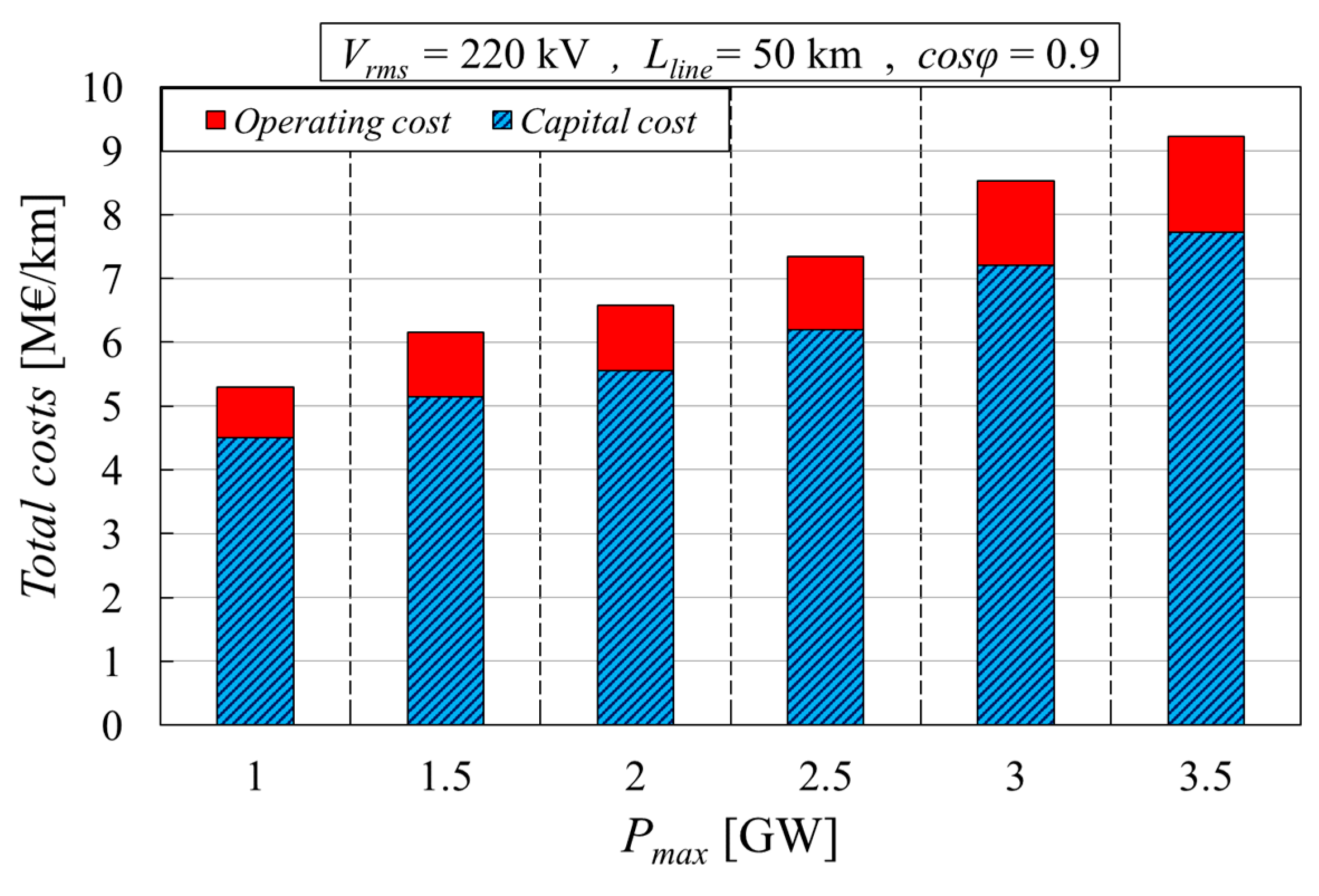
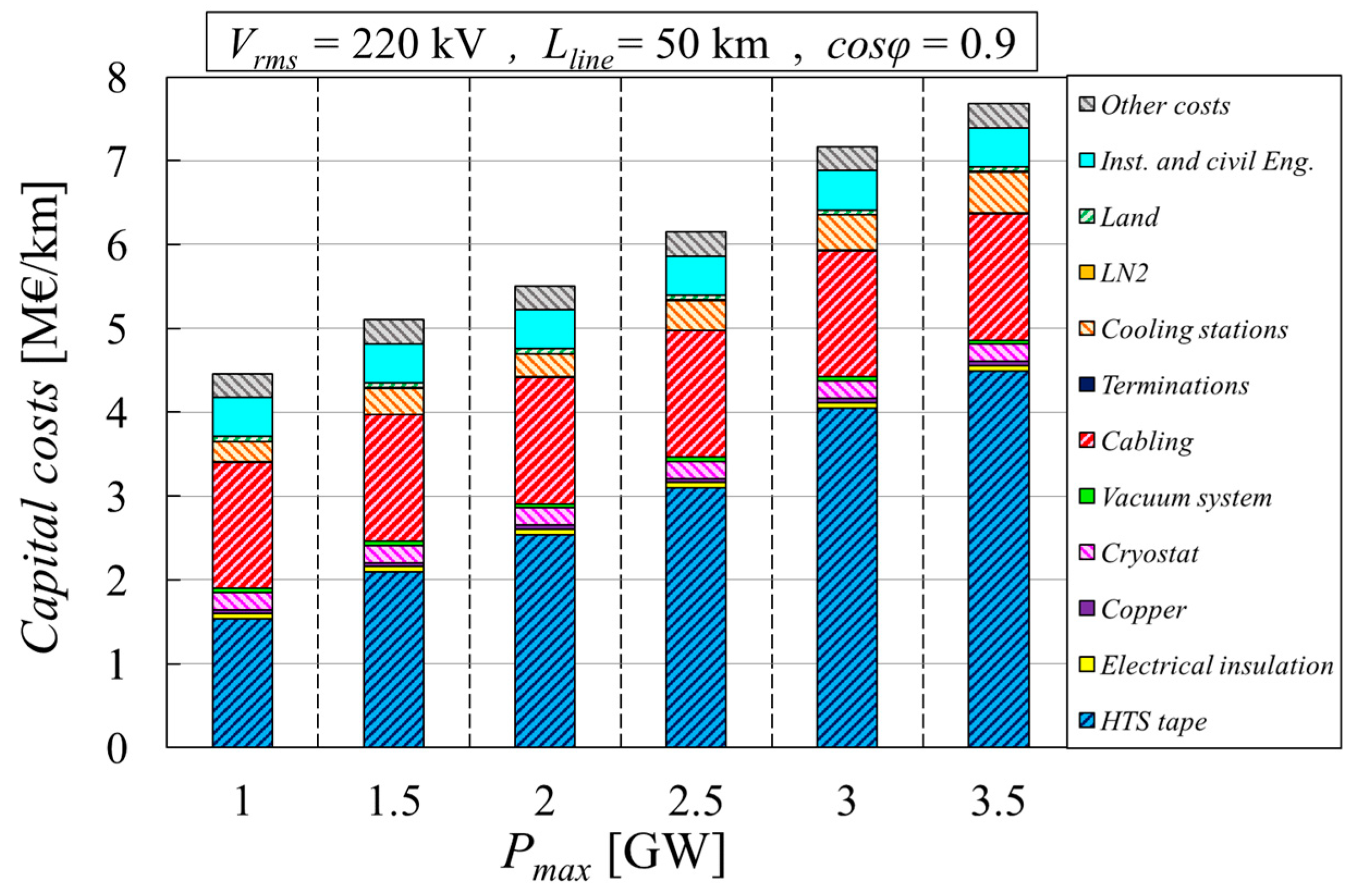
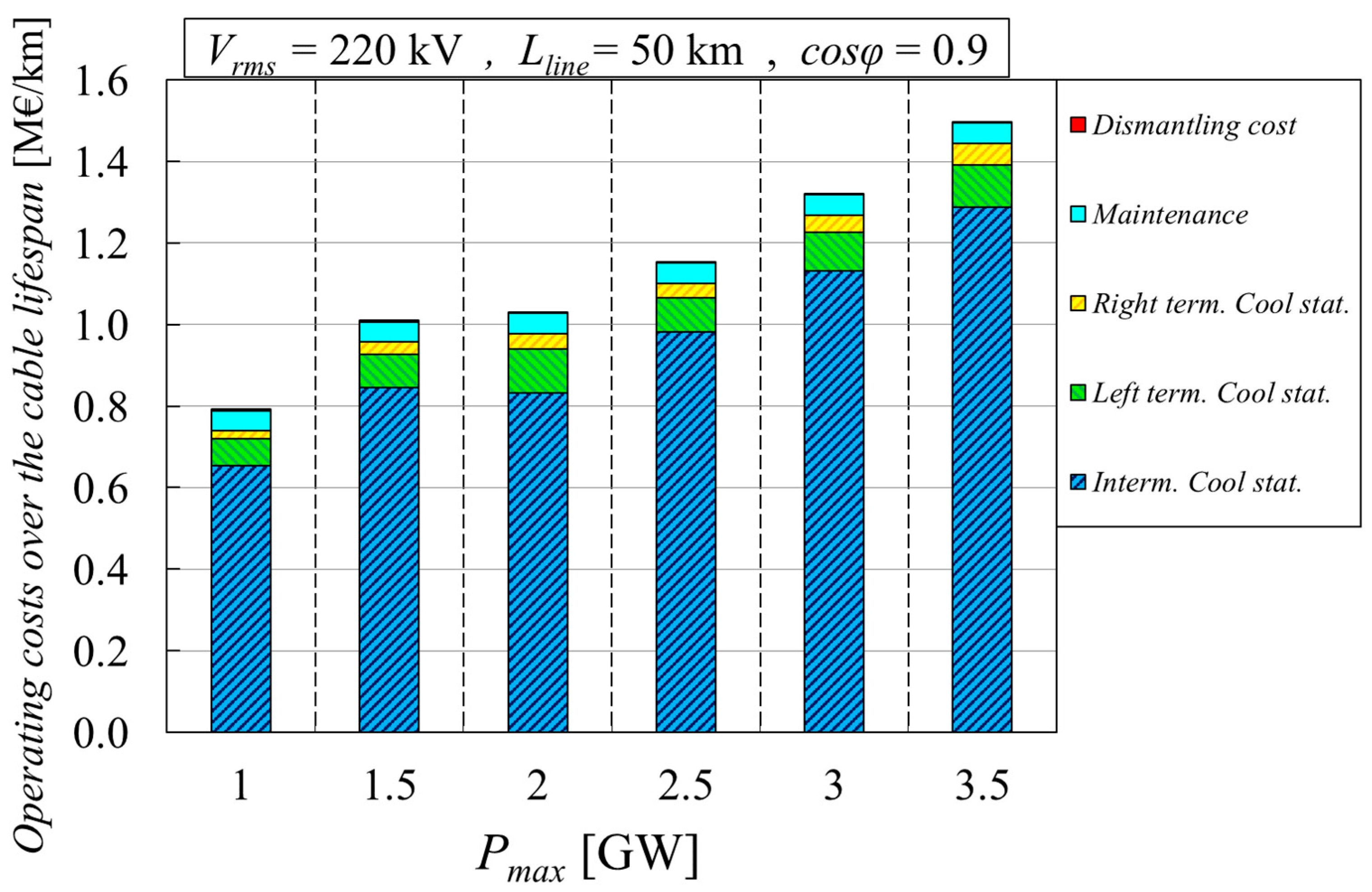
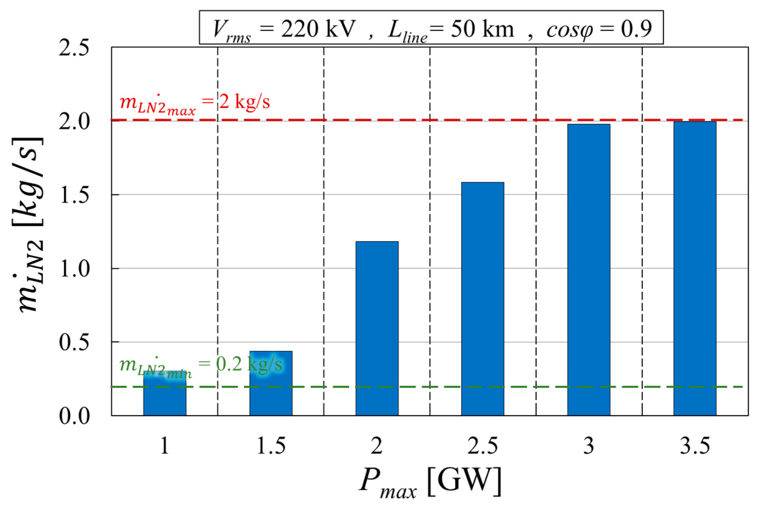
8.1. Impact of the Cable’s Active Power

In this analysis, a 50 km long cable was connected to a load with a $cos\phi$ equal to 0.9 at a voltage level of 220 kV. OSCaR was run while varying the peak active power from 1 GW to 3.5 GW in increments of 0.5 GW, computing the optimal set of system variables and the corresponding cost indexes and cable configuration for each case. $P_{max}$ refers to the maximum power delivered by the cable during its yearly operation. The power trend profile in Figure 4 (blue curve) was thus scaled based on the value of $P_{max}$.

Compared with the medium voltage lines discussed in [35,36], longer line lengths were investigated here, as the authors considered that HVAC cables might be more suitable for these extended distances.

Figure 6 shows the total costs per kilometer of the line (expressed in EUR M/km) for the various cases, distinguishing between the overall capital and operating costs. As expected, the costs increased with the power, although not linearly. Compared with the 1 GW value, the costs per kilometer, and therefore the costs of the entire line, increased by 21% when the power was doubled and by 60% when it was tripled. When neglecting the practical challenges of managing extremely high-power lines and sizing their ancillary devices, the economic benefit of having more powerful individual lines rather than multiple less-powerful cables in parallel is evident. Overall, the estimated cost of the proposed HTS lines varied from EUR 5.3 M/km for the 1 GW scenario to EUR 9.2 M/km for the 3.5 GW case. Readers should consider these results as qualitative, given that they were derived from several approximations and user-defined parameters available or hypothesized by the authors in Section 7.

Furthermore, it can be seen that the ratio between the capital and operating costs was strongly unbalanced toward the first values. In fact, the sum of the operating costs over the entire estimated lifespan of the cable (yr = 40 years) contributed only between 15% and 16.4% of the total costs.

Then, Figure 7 expands the different contributions to the capital costs shown in Figure 6. The main capital costs, in order of their contribution to the total costs, were related to the purchase of the superconducting tapes, the cabling of the various materials together, the civil engineering work to install the cable, the cooling stations, the costs of the accessory components (categorized as other costs), and the cost of the cryostat. The remaining cost terms were minor if not negligible, such as the costs for terminations, which have been divided in Figure 7 by the entire cable length and therefore yielded minimal results.

It is worth noting that the impact of the cost of the superconducting material over the total capital costs increased as the power increased (from 27% at 1 GW up to 58% at 3.5 GW), while the cabling costs were instead considered fixed per unit length.

Moreover, Figure 8 expands the different contributions to the operating costs shown in Figure 6. Note that these costs are the sum of all the operating expenses which occurred during the cable’s lifespan. It was decided to separate the costs of the intermediate cooling stations from those of the termination ones as they were differently sized, although Equation (25) groups them into a single term $C_{coo{l}_{op}}$. It can be observed that the operating cost for the cooling station on the arbitrarily designated left side of the cable was higher than that on the right side. This is because the left termination station must manage the nitrogen flow coming from the annular gap (referencing Figure 2), which absorbs the additional contribution $Q_{cryo}$.

Clearly, the operating cost of the intermediate cooling stations is the most significant cost, as it includes the costs of multiple stations. Specifically, for the cases analyzed, the number of intermediate cooling stations ($n_{stat}$) ranged from 6 (for the 2 GW case) to 9 (for 2.5–3.5 GW), corresponding to the upper limit imposed on this variable for a 50 km-long line. Notably, the operating cost for the termination stations was slightly higher in the 2 GW case compared with the others. In fact, with fewer intermediate stations over the same cable length, the modular cable segments were longer, resulting in more heat absorption by the fluids in each segment, including those connected to the termination stations. Lastly, maintenance and dismantling costs together corresponded to approximately 5% of the total operating costs, thus being almost negligible.

Figure 9 illustrates the trend of losses and heat inputs for the different cases analyzed. The losses presented are calculated along the entire length of the line, with AC losses in the HTS tapes and thermal inputs from the cryostat being the primary contributors. As expected, the trend of operating costs in Figure 8 closely follows the trend of losses, since maintenance and dismantling costs were assumed to be constant per unit cable length. The cost of electricity for pumping the cryogenic fluid, included in Equation (25), had minimal impact, contributing approximately 1% to the total operating costs.

An exception to the proportionality between the operating costs and losses occurred when comparing the 1.5 GW and 2 GW cases. Indeed, the 1.5 GW case showed slightly lower total operating costs than the 2 GW case, despite having slightly higher total losses. This discrepancy can be explained as follows. The losses shown in Figure 9 are calculated assuming that the cable carried a constant power equal to $P_{max}$ for its entire lifespan, represented by the dotted horizontal line in Figure 4. However, this condition did not match the real scenario under which the operating costs were recalculated at the end of the optimization process, as explained in Section 3.4. Figure 10 depicts the trend of hourly operating costs per unit length throughout the year, focusing on the 1.5 and 2 GW cases only and considering the real time-varying cable power, shown as the blue curve in Figure 4. As observed, while the costs at peak power (case at h = 0) reflected the trend in Figure 9, the ratio between the two cases varied over the year until it reversed. This is because the AC losses in the superconductor, which significantly contributed to the total losses and the corresponding operating costs, did not vary linearly with the power or current flowing in the tapes but followed the functions in Equations (31) and (33), which are also dependent on the temperature and critical current. By summing the costs incurred throughout the year in the different time intervals (i.e., integrating the profiles in Figure 10 over time), the operating costs shown in Figure 8 were reproduced and thus justified.

Furthermore, Figure 9 also explains the rising trend of the capital costs of the cooling stations with the power shown in Figure 7, given that these must be sized proportionally to the growing losses they must manage and therefore require greater investment costs.

The main economic indexes discussed thus far are directly dependent on their corresponding optimized cable structures. Therefore, it is of interest to show the main characteristics of the computed geometries.

Figure 11 displays the dimensions of some selected coaxial layers within the cable, as determined by the optimization process under the same conditions as the other figures shown in this section. The blue-purple bars represent the radii of the selected layers, and the values of these bars refer to the left axis of the figure. Specifically, the optimized radius of the former $R_f$ increased with the power, ranging from 1 cm to 2.5 cm. The inner and outer radii of the annular gap are also shown. From their difference, the optimized thickness of the annular gap $t_{an}$ can be deduced, which increased from 1 cm to 2.4 cm and thus increased the power. Additionally, the trend of the external radius of the cryostat, representing the total radial size of the cable, is illustrated. This dimension ranged from 10.7 cm for the 1 GW case to 12.6 cm for the 3 GW and 3.5 GW cases. Thus, the cable encumbrance remained quite limited despite the high power and voltage levels involved. The small variation in the cryostat’s outer radius among the different cases explains the trend of $Q_{cryo}$ in Figure 9; as shown in Equation (37) it depends on $R_{cry{o}_{ext}}$ (as well as $R_{cry{o}_{int}}$) and the nitrogen temperature in the annulus, which could only vary by a few degrees Kelvin between the different cases.

Then, Figure 11 also shows the optimized thicknesses of the concentric insulation layers, depicted as red-yellow bars, whose values refer to the right axis of the figure. The inner insulating layers were thicker than the outermost ones, which directly followed from Equations (11) and (12), because these layers must sustain the same $V_{rms}$ level as the others while having lower inner radii. For the same reason, as $P_{max}$ increased, the thickness of these layers decreased, a trend previously observed for medium-voltage coaxial cables [35,36].

It is also interesting to examine the optimized number of HTS tapes wound in parallel around each layer as $P_{max}$ varied, as shown in Figure 12. Up to the 2 GW case, each phase consisted of a single layer, but starting from the 2.5 GW case, the innermost phase required two layers to meet the constraints. The difference of one unit notable in some cases between the two parallel layers of phase 1 was due to the numerical approximation of the round function in Equation (17) and the slightly larger circumference of layer 2 compared with layer 1, as layer 2 was wound around layer 1.

Overall, the number of tapes per phase increased with the power. However, there was a decrease in the passage between the 2 GW and 2.5 GW cases, as dividing the HTS tapes of phase 1 into two layers required winding them into smaller circumferences, which in turn also reduced the circumferences of the inner and outer layers (from which a slight reduction in the values of $R_f$ and $R_{cry{o}_{ext}}$ followed for the 2.5 GW case compared with the 2 GW case). As the circumferences of the outermost HTS layers reduced, the number of tapes composing them had to decrease.

Figure 13 presents the optimized system variable $\sqrt{2}\left|\underset{\_}{I_{tap{e}_{i,1}}}\right|/I_c\left(T_{HT{S}_{max}}, {\left|B\right|}_{i,1}, {\theta }_{i,1}\right)$ for the three phases as red-yellow bars, with values displayed on the right axis. For all powers and phases, this parameter fell within the range specified in Table 5, indicated by the red dashed horizontal lines.

The corresponding $I_{c_{77K_i}}$ values for the same phases are also displayed in Figure 13 as blue-purple bars whose values refers to the left axis. As expected, OSCaR suggested using lower-quality tapes for the outermost phases, which had larger circumferences and therefore required more HTS tapes, preventing their excessive underloading. This proportionality seemed to reverse for phase 1 from the 2 GW case onward. However, this might be explained by the fact that the total number of tapes in phase 1 increased significantly when reaching $P_{max}$ = 2.5 GW, requiring two parallel layers, as shown in Figure 12. In fact, while the current increased by 25% between 2 GW and 2.5 GW, the number of tapes almost doubled, with a consequent impact on the optimized $I_{c_{77K_i}}$ and $\sqrt{2}\left|\underset{\_}{I_{tap{e}_{i,1}}}\right|/I_c\left(T_{HT{S}_{max}}, {\left|B\right|}_{i,1}, {\theta }_{i,1}\right)$. When approaching the highest power level, the critical current proposed for all phases seemed to be uniform with the values closer to the upper limits, trying to maintain the ratio with the operating current being relatively low.

It is worth noting how for the 1 GW case, the solver did not meet the constraint for the minimum $I_{c_{77K_i}}$ for phase 3, whose limits are reported in Table 5 and indicated by blue dashed horizontal lines. This could be due to an incorrect combination of user-defined parameters and constraints proposed by the authors in Section 7, leading to the selection of particularly poor-performing HTS tapes for this outer phase. Nonetheless, this is the only constraint not respected in all of the parametric analyses shown.

By combining the values from Figure 12 and Figure 13, it can be concluded that the solver suggests using better-performing tapes in the phases where they are needed in lower quantities. However, understanding how the capital cost of the tapes shown in Figure 7 is divided between the various phases is not straightforward. This allocation depends on factors such as the radii of the HTS phases, their winding angles, and the quantitative discounting process. To provide readers with a range of total HTS tape lengths required for a 50 km line, these varied from 7000 km for the 1 GW case to 12,000 km for the 3.5 GW case. These quantities likely exceed the current production capabilities of most manufacturers but offer an insight into the scale of investment needed for the future application of superconducting cable technology.

Finally, Figure 14 shows the optimized values for the LN2 mass flow rate $\dot{m_{LN2}}$ for the various cases analyzed. The flow rate increased with the power, staying within the user-defined limits (indicated by dashed horizontal lines). This was expected, as managing higher thermal inputs requires a greater flow of coolant, considering that the transport current rises when the cable is not divided into significantly more segments ($n_{stat}$ only varied from 6 to 9 units).

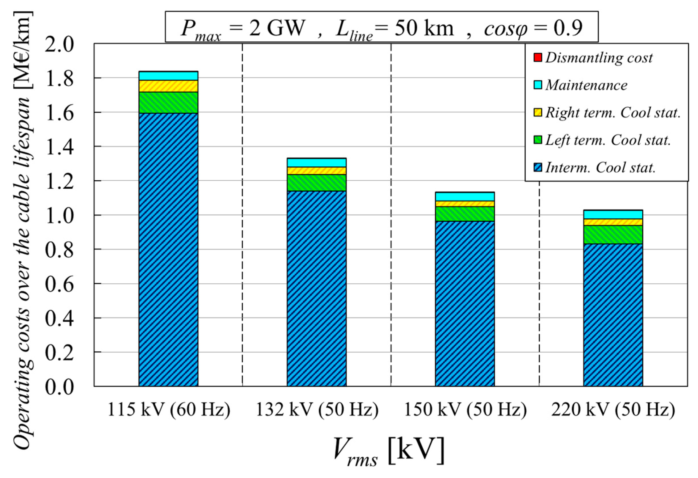
8.2. Impact of the Cable’s Voltage Level

In this study, a 50 km-long cable with a rated maximum power of 1 GW was connected to a load with a $cos\phi$ equal to 0.9. For this parametric analysis, the tool compared different voltage levels selected by the authors among those considered most significant. Since a precise classification of HVAC levels is not well defined globally, the authors chose to investigate some known maximum and minimum limits. For example, 220 kV is considered the maximum limit for high voltage-class lines in several parts of Europe [69,70], while higher voltages are classified as extremely or extra-high voltages. Extremely high voltages were excluded from this investigation as they tend to complicate the construction of a transmission line and do not fully exploit the high-current capabilities of superconducting materials. The results shown here for the 220 kV case clearly coincide with those presented in the previous section for the same case. The lower limit of this parametric analysis was set equal to the lower limit for high voltage-class lines according to American standards: 115 kV [71]. To be consistent, the corresponding frequency value was also adjusted to 60 Hz to follow American regulations. Additionally, some intermediate values, such as 132 kV (the level used in various countries, including the UK) and 150 kV (the level used in various countries, including Switzerland), were selected.

Figure 15 illustrates the capital cost contributions per unit cable length for the various voltage scenarios described. As expected, for the same power level, capital costs increased as the voltage decreased, with the 115 kV case incurring 53% higher investment costs than the 220 kV case. However, it is important to note that the cost calculation did not account for certain devices, such as transformers, for which no techno-economic correlation was found. These devices typically have costs proportional to the voltage level they need to handle and can impact the overall budget.

The main index cost increase corresponded to the HTS tapes, which were needed in greater quantities as the voltage decreased. Specifically, the number of overlaying layers composing phase 1 (${nl}_3$) was equal to three for the 115 kV case, ${nl}_3$ = 2 for the 132 kV and 150 kV cases, and ${nl}_3$ = 1 for the 220 kV case, leading to a nearly proportional number of tapes in phase 1. While the outer phases in the lower-voltage cases still consisted of a single layer, these tapes had to carry significantly more current, prompting the solver to use higher-performing and more expensive coated conductors.

The insulation cost remained relatively constant across different cases, since the thickness of the insulating layers did not vary significantly when changing the voltage. This “unexpected” regularity was due to theses thicknesses being mainly determined by the requirements for managing the lightning impulse conditions and not the AC nominal voltage levels. Different user-defined parameters in Section 7.2 might reach different conclusions.

Then, Figure 16 shows the contributions to the operating costs per unit length of the line, calculated over the entire cable lifespan, for the same voltage cases as those in Figure 15. As concluded for the parametric analysis carried out in Section 8.1, the operating costs were primarily due to the losses managed by the cooling system. These losses increased as the voltage level decreased because the operating current rose proportionally at fixed transport power values. However, the losses did not increase linearly with the current, which was particularly significant in the 115 kV case. Specifically, the AC losses in the superconductor, which were the largest contribution to the total losses, were 4.3 times higher than in the 220 kV case when $V_{rms}$ was 115 kV, 2.4 times higher when $V_{rms}$ was 132 kV, and 1.8 times higher when $V_{rms}$ was 150 kV. Moreover, in the 115 kV case, setting the frequency to 60 Hz led to a proportional higher $Q_{AC}$ compared with the 50 Hz cases, which also affected the insulation losses. As for $Q_{ins}$, these values decreased as the voltage decreased. However, their impact was limited, ranging from 4% to 11% between 115 kV and 220 kV.

Adding the capital and the operating costs resulted in a total cost per unit of length sized for $P_{max}$ = 2 GW ranging from EUR 10.3 M/km for the 115 kV scenario to EUR 6.6 M/km for the 220 kV scenario. This would suggest that moving toward higher voltages is also advantageous for superconducting cables, similar to conventional high-power cables. However, it is important to remember that the presented results do not include the cost of transformers.

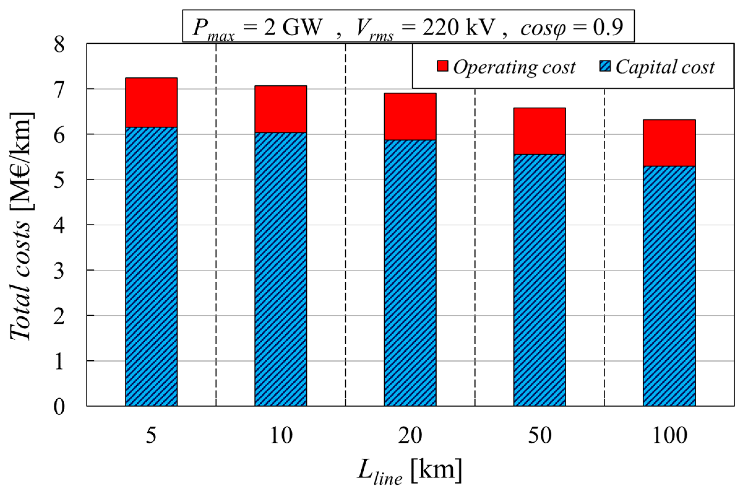
8.3. Impact of the Line Length

In this last analysis, a cable with a rated maximum power of 2 GW and a $V_{rms}$ level of 220 kV was connected to a load with a $cos\phi$ equal to 0.9. The line length was varied between 5 km and 100 km to check the main techno-economic trends in this range.

Figure 17 shows the model’s output for the total costs per unit of line length for the values of $L_{line}$ considered, distinguishing between the overall capital and operating costs. The economic convenience of developing longer HVAC superconducting lines compared with shorter lines appears to be limited though not negligible. Furthermore, the cost reduction was more pronounced than in the case of medium-voltage cables discussed in [35], as the quantitative discounting approach was not considered in the previous publication. Extending the line length from 5 km to 100 km resulted in approximately a 13% reduction in the total costs. The ratio of operating to capital costs consistently remained between 15% and 16%.

It is reasonable to expect that the cost reduction with an increasing $L_{line}$ will eventually saturate once certain lengths are achieved, as the quantities of the discounted terms would reach their respective discount limits $d_{{max\%}_x}$. However, up to 100 km, this saturation trend was not observed, in contrast to the findings in [35].

Lastly, Figure 18 shows the trend of the optimized value of $n_{stat}$ with the cable length as blue bars whose values are reported on the left axis. These varied from 0 units for the shortest line up to 16 units for the longest one. Since the distances on the x axis of Figure 18 are not proportional, it can be difficult to visualize that the ratio between the number of intermediate cooling stations and the length of the line is not exactly constant. This is better displayed by the red bars in Figure 18 (referenced on the right axis), which represent the distance between adjacent stations or the length of each modular cable segment $d_{stat}$. This distance varied between 5 km, the minimum value set in Table 5, and 7.1 km.

9. Conclusions

This work presents an innovative approach for the techno-economic assessment of coaxial HVAC transmission cables made with HTS tapes and cooled with liquid nitrogen using a double-sided cooling option with two concentric coolant channels inside the cable. The proposed method is based on the OSCaR optimization tool, adapted here for high-voltage transmission lines rated for extremely high power values. Despite the necessary insulation thicknesses required to handle the voltage levels, the coaxial configuration is believed to offer advantages over other cable designs, maintaining a limited radial size compared with the powers involved. To the authors’ knowledge, this paper is the first to present a techno-economic analysis model specifically applied to this type of superconducting cable.

This work aimed to identify the cable structure which minimized the cable system’s costs, allowing users to select the operating conditions of the line and conduct comprehensive and time-efficient parametric analyses. Mathematically, this was achieved through a constrained multi-variable minimization process for the cable system’s cost solved via a genetic algorithm in MATLAB software v2022b. Ample space was given in the article in detailing the methodological approach so as to allow readers to understand the relationships between the variables involved and potentially adapt the tool to their specific needs. The thermo-hydraulic and electro-magnetic models were included in the model via numerical and analytical correlations with proven effectiveness, ensuring the tool comprehensively addressed the key technical factors which must be considered when sizing a cable system.

A grading approach for the critical current of the HTS tapes used in various phases was introduced in the tool, a technique which, to the authors’ knowledge, has not yet been applied to superconducting cables. The cost per unit length of the coated conductors was optimized according to the thermo-electro-magnetic conditions to which they were subjected in the individual concentric layers. This enabled optimization of both the quantity and quality of the superconducting tape used in the cable, a factor which is known to significantly impact the total costs. The selected system variables included the number of parallel HTS layers per phase, the winding angle of the tapes in each layer, the radius of the central former, the thickness of the annular gap for the liquid nitrogen counterflow, the nitrogen mass flow rate valid in both channels, the number of intermediate cooling stations to maintain the temperature and pressure limits in the coolant, and finally the ratio $\sqrt{2}\left|\underset{\_}{I_{tap{e}_{i,1}}}\right|/I_c\left(T_{HT{S}_{max}}, {\left|B\right|}_{i,1}, {\theta }_{i,1}\right)$, which in turn determined the characteristics of the tapes used in each phase (in terms of the critical current at 77 K and self-field $I_{c_{77K_i}}$) and the corresponding cost per unit length.

The constraints imposed on the optimized geometry concerned the temperature and pressure levels of the nitrogen within the two channels, ensuring it remained in a liquid state in each modular cable segment. Additionally, the geometry of each superconducting layer was adjusted to ensure a uniform current distribution between the layers of the same phase and among the phase currents. Then, the $I_{c_{77K_i}}$ value of the tapes in each layer was kept within reasonable limits based on the estimated current capabilities of tape manufacturers.

Overall, the cost function considered here distinguishes between operating costs and capital costs. The former are further divided between the costs for operating the cooling stations, line maintenance, and its dismantling. The capital costs are distinguished between the costs for purchasing the HTS tapes, insulating material, and cryostat, the cabling of all materials into the final architecture, the purchase of the cooling stations (distinguishing between the intermediate and termination ones, which are different sizes), the cable terminations, and the vacuum system. Here, the capital costs also included the purchase of land for underground line installation, the copper for the neutral layer conductor, and additional capital costs for the cable installations, their commissioning, and the costs referred to ancillary devices. These last cost indexes were not present in previous OSCaR versions. These terms, though not decisive for the specific cable configuration analyzed, could impact other designs which might be investigated in the future using OSCaR tool and are therefore included in this comprehensive document.

Furthermore, other improvements of this version of the tool comprise the quantitative discounts applied to the capital costs for the selected cable system elements based, for example, on the quantity of superconducting tape required or the total number of cooling stations to be purchased. Moreover, the operating costs are computed by considering a time-varying power curve over a year (and therefore over the entire device lifespan), rather than assuming a constant maximum power. These approaches are expected to yield more accurate and realistic cable cost calculations.

Additionally, the user-defined parameters necessary for calculation were updated for the HVAC cases compared with the previous medium-voltage case [36], enhancing the tool’s relevance for high-voltage applications, such as the use of a more efficient insulating material, Tyvek PE, compared with the conventional PPLP.

The effectiveness and versatility of the developed tool are demonstrated through relevant parametric analyses. The results of these analyses should be considered qualitative, providing general trends for relevant design parameters. Indeed, the values reported were heavily dependent on the user-defined parameters and the availability of reliable data. Users with different data sets can apply the comprehensive methodology outlined in this work to obtain more quantitative results tailored to their specific needs.

As a first example, the model was applied to estimate the costs of superconducting cables for transmitting extremely high power values (between 1 GW and 3.5 GW) at a voltage of 220 kV, which was chosen as the upper limit for high-voltage applications, as analyzing extra-high voltage levels might not be ideal for maximizing the potential of the superconducting technology. These power levels, which are challenging for current networks, could become advantageous with future grid developments and increased localized electricity production and demand.

In the parametric analysis of a 50 km line connected to load with a $cos\phi$ equal to 0.9, the overall cable system cost ranged from EUR 5.3 M/km for the 1 GW case to EUR 9.2 M/km for the 3.5 GW case. It can be concluded that single high-power cables are more cost-effective than installing multiple lower-power cables in parallel. However, these results do not account for the cost of some accessory components, such as transformers.

The operating costs over the cable’s lifespan (40 years) were limited to 15–16% of the total costs, primarily due to the operation of the cooling and pumping stations. These costs closely followed the trend of losses calculated based on the real-time varying power curve of the cable and not just its maximum power condition. Regarding the losses, those ones due to AC currents in the superconducting tapes and the thermal inputs entering the cryostat from outside were the most relevant ones. The capital costs mainly depended on the cost of the HTS tapes, the cabling process, the cryostat, and the civil engineering works for installation. The cable’s radial size was reasonably contained in all cases analyzed, varying from 10.7 cm to 12.6 cm for the higher-power case and being significantly smaller than those ones for conventional lines or even other superconducting architectures. The solver suggests using coated conductors with lower electric characteristics (in terms of homogeneity of the critical current along the entire length purchased) for phases realized with more tapes, assuming perfectly balanced AC currents. This occurred for the outermost phases, characterized by a greater number of tapes wound side-by-side over wider circumferences. However, the trend was not linear, with the number of parallel layers increasing stepwise (and thus with a stepwise increase in the number of tapes per phase), such as the doubling of the innermost phase (phase 1) from the 2 GW case to the higher-power cases.

Subsequently, a parametric analysis was conducted on a 50 km cable transmitting 2 GW at different voltage and frequency levels taken as the most significant levels in worldwide grids: 115 kV/60 Hz, 132 kV/50 Hz, 150 kV/50 Hz, and 220 kV/50 Hz. As expected, lowering the voltage increased the costs, primarily due to higher expenses for superconducting tapes and managing greater AC losses. The total system costs rose by about 53% when the voltage was nearly halved.

Finally, a parametric analysis evaluated the cost-effectiveness of different HVAC transmission line lengths. For a 2 GW cable at 220 kV, considering lengths between 5 km and 100 km resulted in savings of approximately 13% for the longest lines compared with the 5 km reference case. For the specified power level and the user-defined parameters, the tool recommended several intermediate cooling stations spaced between 5 km (corresponding to the minimum distance imposed by the authors for adjacent stations) and 7.1 km apart.

The approach proposed in this study enables identification of the applicative scenarios within electricity grids where the use of HTS HVAC cables would be more beneficial, providing valuable insights for the cables design phase as well. The comprehensive methodology described here, which the authors consider to be the most significant contribution of this work, is intended to be applied to other superconducting and conventional cable configurations to identify conditions of potential techno-economic convenience.

References

1. Garwin, R.L.; Matisoo, J. Superconducting lines for the transmission of large amounts of electric power over great distances. Proc. IEEE 1967, 55, 538–548. [Google Scholar] [CrossRef]
2. Forsyth, E.B.; Thomas, R.A. Performance summary of the Brookhaven superconducting power transmission system. Cryogenics 1986, 26, 599–614. [Google Scholar] [CrossRef]
3. Kim, D.W.; Jang, H.-M.; Lee, C.-H.; Kim, J.-H.; Ha, C.-W.; Kwon, Y.-H.; Kim, D.-W.; Cho, J.-W. Development of the 22.9-kV class HTS power cable in LG cable. IEEE Trans. Appl. Supercond. 2005, 15, 1723–1726. [Google Scholar] [CrossRef]
4. Sim, K.; Kim, S.; Cho, J.; Kim, D.; Kim, C.; Jang, H.; Sohn, S.; Hwang, S. DC critical current and AC loss measurement of the 100 m 22.9 kV/50 MVA HTS cable. Physica C 2008, 468, 2018–2022. [Google Scholar] [CrossRef]
5. Lee, S.; Yoon, J.; Lee, B.; Yang, B. Modeling of a 22.9 kV 50 MVA superconducting power cable based on PSCAD/EMTDC for application to the Icheon substation in Korea. Phys. C Supercond. Its Appl. 2011, 471, 1283–1289. [Google Scholar] [CrossRef]
6. Lee, C.; Hyukchan, S.; Youngjin, W.; Youngwoong, K.; Cheolhwi, R.; Minwon, P.; Masataka, I. Progress of the first commercial project of high-temperature superconducting cables by KEPCO in Korea. Supercond. Sci. Technol. 2020, 33, 044006. [Google Scholar] [CrossRef]
7. Takahashi, T.; Suzuki, H.; Ichikawa, M.; Okamoto, T.; Akita, S.; Mukoyama, S.; Ishii, N.; Kimura, A.; Yasuda, K. Demonstration and verification tests of 500 m long HTS power cable. IEEE Trans. Appl. Supercond. 2005, 15, 1823–1826. [Google Scholar] [CrossRef]
8. Maruyama, O.; Ohkuma, T.; Masuda, T.; Ashibe, Y.; Mukoyama, S.; Yagi, M.; Saitoh, T.; Hasegawa, T.; Amemiya, N.; Ishiyama, A.; et al. Development of 66 kV and 275 kV class REBCO HTS power cables. IEEE Trans. Appl. Supercond. 2013, 23, 5401405. [Google Scholar] [CrossRef]
9. Masuda, T.; Watanabe, M.; Mimura, T.; Tanazawa, M.; Yamaguchi, H. The 2nd in-grid operation of superconducting cable in Yokohama project. J. Phys. Conf. Ser. 2020, 1559, 012083. [Google Scholar] [CrossRef]
10. Li, J.; Zhang, L.; Ye, X.; Xia, F.; Cao, Y. Demonstration Project of 35 kV/1 kA Cold Dielectric High Temperature Superconducting Cable System in Tianjin. IEEE Trans. Appl. Supercond. 2020, 30, 5400205. [Google Scholar] [CrossRef]
11. Zong, X.H.; Han, Y.W.; Huang, C.Q. Introduction of 35-kV kilometer-scale high-temperature superconducting cable demonstration project in Shanghai. Superconductivity 2022, 22, 100008. [Google Scholar] [CrossRef]
12. Stemmle, M.; Merschel, F.; Noe, M.; Hobl, A. AmpaCity—Installation of advanced superconducting 10 kV system in city center replaces conventional 110 kV cables. In Proceedings of the IEEE International Conference on Applied Superconductivity and Electromagnetic Devices, Beijing, China, 25–27 October 2013; pp. 323–326. [Google Scholar]
13. Soika, R.; Granados Garcia, X.; Cascante Nogales, S. ENDESA supercable, a 3.2 kA, 138 MVA, medium voltage superconducting power cable. IEEE Trans. Appl. Supercond. 2011, 21, 972–975. [Google Scholar] [CrossRef]
14. Volkov, E.P.; Vysotsky, V.S.; Firsov, V.P. First Russian long length HTS power cable. Physica C 2012, 482, 87–91. [Google Scholar] [CrossRef]
15. Allais, A.; Saugrain, J.-M.; West, B.; Lallouet, N.; Caron, H.; Ferandelle, D.; Terrien, L.; Bouvier, G.; Hajiri, G.; Berger, K.; et al. SuperRail–World-First HTS Cable to be Installed on a Railway Network in France. IEEE Trans. Appl. Supercond. 2024, 34, 4802207. [Google Scholar] [CrossRef]
16. Magnusson, N.; Allais, A.; Angeli, G.; Bouvier, G.; Bruzek, C.E.; Candido, J.; Creusot, C.; Gammelsæter, M.; Garofalo, E.; Gömöry, F.; et al. SCARLET—A European Effort to Develop HTS and MgB2 Based MVDC Cables. IEEE Trans. Appl. Supercond. 2024, 34, 5400205. [Google Scholar] [CrossRef]
17. Maguire, J.F.; Folts, D.; Yuan, J.; Henderson, N.; Lindsay, D.; Knoll, D.; Rey, C.; Duckworth, R.; Gouge, M.; Wolff, Z.; et al. Status and progress of a fault current limiting HTS cable to be installed in the Con Edison grid. Adv. Cryog. Eng. 2009, 55A, 445–452. [Google Scholar]
18. Maguire, J.F.; Yuan, J.; Romanosky, W.; Schmidt, F.; Soika, R.; Bratt, S.; Durand, F.; King, C.; McNamara, J.; Welsh, T.E. Progress and status of a 2G HTS power cable to be installed in the Long Island Power Authority (LIPA) grid. IEEE Trans. Appl. Supercond. 2011, 21, 961–966. [Google Scholar] [CrossRef]
19. Schmidt, F.; Allais, A. Superconducting cables for power transmission applications—A review. In Proceedings of the Workshop on Accelerator Magnet Super-Conductors (WAMS) Proceedings, Archamps, France, 22–24 March 2004; p. 352. [Google Scholar]
20. Malozemoff, A.P.; Yuan, J.; Rey, C.M. High-temperature superconducting (HTS) AC cables for power grid applications. In Superconductors in the Power Grid Materials and Applications; Woodhead Publishing Series in Energy; Woodhead Publishing: Cambridge, UK, 2015; pp. 133–188. [Google Scholar]
21. Ren, L.; Tang, Y.; Shi, J.; Li, L.; Li, J.; Cheng, S.C. Techno-Economic Feasibility Study on HTS Power Cables. IEEE Trans. Appl. Supercond. 2009, 19, 1774–1777. [Google Scholar] [CrossRef]
22. Venuturumilli, S.H.; Zhang, Z.; Zhang, M.; Yuan, W. Superconducting Cables-Network Feasibility Study Work Package 3. 2017. Available online: https://www.westernpower.co.uk/downloads-view-reciteme/2152 (accessed on 1 February 2024).
23. Yuan, W.; Venuturumilli, S.; Zhang, Z.; Mavrocostanti, Y.; Zhang, M. Economic Feasibility Study of using High Temperature Superconducting cables in UK’s Electrical Distribution Networks. IEEE Trans. Appl. Supercond. 2018, 28, 5401505. [Google Scholar] [CrossRef]
24. Yu, Z.; Ren, Y.; Cao, B.; Liu, J.; Zhou, Z. Feasibility and Economical Analysis of the Superconducting Cable and Hydrogen Hybrid Transmission Gallery. In Proceedings of the 2020 IEEE International Conference on Applied Superconductivity and Electromagnetic Devices, Tianjin, China, 16–18 October 2020. [Google Scholar]
25. Guarino, R.; Wesche, R.; Sedlak, K. Technical and economic feasibility study of high-current HTS bus bars for fusion reactors. Phys. C Supercond. Its Appl. 2022, 592, 1353996. [Google Scholar] [CrossRef]
26. Ferran, P.C. Economical Study of Electric Power Transmission with Superconducting Lines for HVDC Systems. Ph.D. Thesis, Escola Tècnica Superior d’Enginyeria Industrial de Barcelona, Barcelona, Spain, 2021. [Google Scholar]
27. Long, J.; Ren, L.; Li, J.; Xu, Y.; Shi, J.; Tang, Y. High-Temperature Superconducting Cable Optimization Design Software Based on 2-D Finite Element Model. IEEE Trans. Appl. Supercond. 2022, 32, 4801405. [Google Scholar] [CrossRef]
28. Peng, S.; Cai, C.; Cai, J.; Zheng, J.; Zhou, D. Optimum Design and Performance Analysis of Superconducting Cable with Different Conductor Layout. Energies 2022, 15, 8893. [Google Scholar] [CrossRef]
29. Politano, D.; Sjostrom, M.; Schnyder, G.; Rhyner, J. Technical and Economical Assessment of HTS Cables. IEEE Trans. Appl. Supercond. 2001, 11, 2477–2480. [Google Scholar] [CrossRef]
30. Elsherif, M.; Taylor, P.; Blake, S. Investigating the potential impact of superconducting distribution networks. In Proceedings of the 22nd International Conference on Electricity Distribution, Stockholm, Sweden, 10–13 June 2013; p. 0816. [Google Scholar]
31. Buchholz, A.; Noe, M.; Kottonau, D.; Shabagin, E.; Weil, M. Environmental Life-Cycle Assessment of a 10 kV High-Temperature Superconducting Cable System for Energy Distribution. IEEE Trans. Appl. Supercond. 2021, 31, 4802405. [Google Scholar] [CrossRef]
32. Sadeghi, A.; Seyyedbarzegar, S. An accurate model of the high-temperature superconducting cable by using stochastic methods. Transform. Mag. 2021, 8 (Suppl. 5), 70–76. [Google Scholar]
33. Kloppel, S.; Marian, A.; Haberstroh, C.; Bruzek, C.-E. Thermo-hydraulic and economic aspects of long-length high-power MgB2 superconducting cables. Cryogenics 2020, 113, 103211. [Google Scholar] [CrossRef]
34. Altov, V.A.; Balashov, N.N.; Degtyarenko, P.N.; Ivanov, S.S.; Kopylov, S.I.; Sytnikov, V.E.; Zheltov, V.V. Optimization of Three- and Single-Phase AC HTS Cables Design by Numerical Simulation. IEEE Trans. Appl. Supercond. 2017, 27, 4801606. [Google Scholar] [CrossRef]
35. Musso, A.; Angeli, G.; Bocchi, M.; Ribani, P.L.; Breschi, M. OSCaR: A Cost Analysis of HTS Coaxial Cables With a Novel Optimization Method. IEEE Trans. Appl. Supercond. 2023, 33, 4803516. [Google Scholar] [CrossRef]
36. Musso, A.; Angeli, G.; Bocchi, M.; Ribani, P.L.; Breschi, M. A method to quantify technical-economic aspects of HTS electric power cables. IEEE Trans. Appl. Supercond. 2022, 32, 4803516. [Google Scholar] [CrossRef]
37. Musso, A.; Cavallucci, L.; Angeli, G.; Bocchi, M.; Breschi, M. A conceptual design optimization for a MgB2 DC transmission line. IEEE Trans. Appl. Supercond. 2024, 34, 6200607. [Google Scholar] [CrossRef]
38. de Sousa, W.T.B.; Shabagin, E.; Kottonau, D.; Noe, M. An open-source 2D finite difference based transient electro-thermal simulation model for three-phase concentric superconducting power cables. Supercond. Sci. Technol. 2021, 34, 015014. [Google Scholar] [CrossRef]
39. Kottonau, D.; de Sousa, W.T.B.; Bock, J.; Noe, M. Design Comparisons of Concentric Three-Phase HTS Cables. IEEE Trans. Appl. Supercond. 2019, 29, 5401508. [Google Scholar] [CrossRef]
40. Morandi, A. HTS dc transmission and distribution: Concepts, applications and benefits. Supercond. Sci. Technol. 2015, 28, 123001. [Google Scholar] [CrossRef]
41. Kottonau, D.; Shabagin, E.; de Sousa, W.T.B.; Geisbüsch, J.; Noe, M.; Stagge, H.; Fechner, S.; Woiton, H.; Küsters, T. Evaluation of the Use of Superconducting 380 kV Cable; KIT Scientific Publishing: Karlsruhe, Germany, 2020. [Google Scholar]
42. Colebrook, C. Turbulent Flow in Pipes with Particular Reference to the Transition Region between the Smooth and Rough Pipe Laws. J. Inst. Civ. Eng. 1939, 11, 133–156. [Google Scholar] [CrossRef]
43. Haaland, S.E. Simple and Explicit formulas for friction factor in turbulent pipe flow. J. Fluid. Eng. 1983, 105, 89–90. [Google Scholar] [CrossRef]
44. Nguyen, T.; Lee, W.-G.; Lee, S.-J.; Park, M.; Kim, H.-M.; Won, D.; Yoo, J.; Yang, H.S. A Simplified Model of Coaxial, Multilayer High-Temperature Superconducting Power Cables with Cu Formers for Transient Studies. Energies 2019, 12, 1514. [Google Scholar] [CrossRef]
45. Seog Whan, K.; Jinho, J.; Jeonwook, C.; Joonhan, B.; Hae-jong, K.; Kichul, S. Effect of winding direction on four-layer HTS power transmission cable. Cryogenics 2003, 43, 629–635. [Google Scholar]
46. Jiahui, Z.; Zhenyu, Z.; Huiming, Z.; Min, Z.; Ming, Q.; Weijia, Y. Inductance and Current Distribution Analysis of a Prototype HTS Cable. J. Phys. Conf. Ser. 2014, 507, 022047. [Google Scholar]
47. Jackson, J.D. Classical Electrodynamics; John Wiley & Sons: Hoboken, NJ, USA, 1975. [Google Scholar]
48. Thomas, H.; Marian, A.; Chervyakov, A.; Stückrad, S.; Rubbia, C. Efficiency of superconducting transmission lines: An analysis with respect to the load factor and capacity rating. Renew. Sustain. Energy Rev. 2016, 141, 381–391. [Google Scholar] [CrossRef]
49. Jovcic, D.; Li, P.; Hodge, E.; Fitzgerald, J. Assessment of interconnection options for 1GW remote offshore wind farm utilizing superconducting HVDC cable without offshore platform. In Proceedings of the 41st CIGRE Symposium, Ljubljana, Slovenia, 21–24 November 2021. [Google Scholar]
50. Cullinane, M.; Judge, F.; O’Shea, M.; Thandayutham, K.; Murphy, J. Subsea superconductors: The future of offshore renewable energy transmission? Renew. Sustain. Energy Rev. 2022, 156, 111943. [Google Scholar] [CrossRef]
51. Choi, J.; Cheon, H.-G.; Choi, J.-H.; Kim, H.-J.; Cho, J.-W.; Kim, S.-H. A Study on Insulation Characteristics of Laminated Polypropylene Paper for an HTS Cable. IEEE Trans. Appl. Supercond. 2010, 20, 1280–1283. [Google Scholar] [CrossRef]
52. Kwag, D.S.; Nguyen, V.D.; Baek, S.M.; Kim, H.J.; Cho, J.W.; Kim, S.H. A Study on the Composite Dielectric Properties for an HTS Cable. IEEE Trans. Appl. Supercond. 2005, 15, 1731–1734. [Google Scholar] [CrossRef]
53. Pi, W.; Yang, Q.; Wang, T.; Peng, C.; Wang, Y.; Shi, Q.; Dong, J. Insulation Design and Simulation for Three-Phase Concentric High-Temperature Superconducting Cable under 10-kV Power System. IEEE Trans. Appl. Supercond. 2019, 29, 7700104. [Google Scholar] [CrossRef]
54. Hayakawa, N. Insulation Technologies for HTS Apparatus; ESAS Summer School on HTS Technology for Sustainable Energy and Transport Systems: Bologna, Italy, 2016. [Google Scholar]
55. Norris, W.T. Calculation of hysteresis losses in hard superconductors carrying AC isolated conductors and edges of thin sheets. J. Phys. Appl. Phys. 1970, 3, 489–507. [Google Scholar] [CrossRef]
56. Amemiya, N.; Jiang, Z.; Nakahata, M.; Yagi, M.; Mukoyama, S.; Kashima, N.; Nagaya, S.; Shiohara, Y. AC Loss Reduction of Superconducting Power Transmission Cables Composed of Coated Conductors. IEEE Trans. Appl. Supercond. 2017, 17, 1712–1717. [Google Scholar] [CrossRef]
57. Musso, A.; Breschi, M.; Ribani, P.L.; Grilli, F. Analysis of AC loss contributions from different layers of HTS tapes using the A−V. formulation model. IEEE Trans. Appl. Supercond. 2021, 31, 5900411. [Google Scholar] [CrossRef]
58. Kottonau, D.; Shabagin, E.; Noe, M.; Grohmann, S. Opportunities for High-Voltage AC Superconducting Cables as Part of New Long-Distance Transmission Lines. IEEE Trans. Appl. Supercond. 2017, 27, 5400405. [Google Scholar] [CrossRef]
59. Trevisani, L. Design and Simulation of a Large Scale Energy Storage and Power Transmission System for Remote Renewable Energy Sources Exploitation. Ph.D. Dissertation, University of Bologna, Bologna, Italy, 2006. [Google Scholar]
60. Gouge, M.J.; Lindsay, D.T.; Demko, J.A.; Duckworth, R.C.; Ellis, A.R.; Fisher, P.W.; James, D.R.; Lue, J.W.; Roden, M.L.; Sauers, I.; et al. Tests of tri-axial HTS cables. IEEE Trans. Appl. Supercond. 2005, 15, 1827–1830. [Google Scholar] [CrossRef]
61. Masuda, T.; Ashibe, Y.; Watanabe, M.; Suzawa, C.; Ohkura, K.; Hirose, M.; Isojima, S.; Honjo, S.; Matsuo, K.; Mimura, T. Development of a 100 m, 3-core 114MVA HTSC cable system. Physica C 2002, 372–376, 1580–1584. [Google Scholar] [CrossRef]
62. Mukoyama, S.; Yagi, M.; Ishii, N.; Kimura, H.; Suzuki, H.; Ichikawa, M.; Takahashi, T.; Okamoto, T.; Kimura, A.; Yasuda, K. Demonstration and verification tests of a 500 m HTS cable in the super-ACE project. Physica C 2005, 426–431, 1365–1373. [Google Scholar]
63. Demko, J.A.; Lue, J.W.; Gouge, M.J.; Lindsay, D.; Roden, M.; Willen, D.; Daumling, M.; Fesmire, J.E.; Augustynowicz, S.D. Cryostat vacuum thermal considerations for HTS power transmission cable systems. IEEE Trans. Appl. Supercond. 2003, 13, 1930–1933. [Google Scholar] [CrossRef]
64. Zuijderduin, R. Integration of High-Tc Superconducting Cables in the Dutch Power Grid of the Future. Ph.D. Thesis, Delft University of Technology, Delft, The Netherlands, 2016. [Google Scholar]
65. Herzog, F. Cooling unit for the AmpaCity project—One year successful operation. Cryogenics 2016, 80, 204–209. [Google Scholar] [CrossRef]
66. Preuß, A. Development of High-Temperature Superconductor Cables for High Direct Current Applications. Ph.D. Dissertation, KIT Scientific Publishing, Institut für Technische Physik (ITEP), Karlsruhe, Germany, 2022. [Google Scholar]
67. Hayakawa, N.; Nishimachi, S.; Maruyama, O.; Ohkuma, T.; Liu, J.; Yagi, M. A Novel Electrical Insulating Material for 275 kV High-Voltage HTS Cable with Low Dielectric Loss. J. Phys. Conf. Ser. 2024, 507, 032021. [Google Scholar] [CrossRef]
68. Allen, N.C.; Chiesa, L.; Takayasu, M. Numerical and experimental investigation of the electromechanical behaviour of REBCO tapes. IOP Conf. Ser. Mater. Sci. Eng. 2015, 102, 012025. [Google Scholar] [CrossRef]
69. Weedy, B.M.; Cory, B.I. Electric Power Systems; John Wiley & Sons: Hoboken, NJ, USA, 1998. [Google Scholar]
70. International Energy Agency. Electricity Grids and Secure Energy Transitions—Enhancing the Foundations of Resilient, Sustainable and Affordable Power Systems. November 2023. Available online: https://www.iea.org/reports/electricity-grids-and-secure-energy-transitions/executive-summary (accessed on 1 February 2024).
71. ANSI C84.1-2011; American National Standard for Electric Power Systems and Equipment—Voltage Ratings (60 Hertz). American National Standards Institute: Washington, DC, USA, 2011.
Figure 1. Illustration of the lateral view of a concentric HTS cable, showing some of the parameters selected as system variables (terms colored in bold). This figure is not to scale [38].
Applsci 14 07488 g001
Figure 2. Illustration of a both-sided cooling option with a single intermediate cooling station. The red colored arrows represent the heat sources entering the two cryogenic fluid flows which circulate through the cable.
Applsci 14 07488 g002
Figure 3. Temperature trends in the two LN2 counter-flows and for all HTS layers along a generic cable segment between adjacent cooling stations. This figure is not to scale.
Applsci 14 07488 g003
Figure 4. Trend of the normalized active power transferred by the line over a year adopted in this work. The yellow area highlights the overestimation of energy compared with the assumption that the cable operates at its full capacity over the whole year.
Applsci 14 07488 g004
Figure 5. Representative diagram of the quantitative discounting approach used for individual cost indexes in this work. This figure is not to scale.
Applsci 14 07488 g005
Figure 6. Total cost per kilometer of a cable, varying the maximum active power transferred. The cases considered had V r m s = 220 kV, c o s φ = 0.9, and L l i n e = 50 km.
Applsci 14 07488 g006
Figure 7. Capital costs per kilometer of cable, varying the maximum active power transferred. The cases considered had V r m s = 220 kV, c o s φ = 0.9, and L l i n e = 50 km.
Applsci 14 07488 g007
Figure 8. Operating costs per kilometer of cable, varying the maximum active power transferred. The cases considered had V r m s = 220 kV, c o s φ = 0.9, and L l i n e = 50 km.
Applsci 14 07488 g008
Figure 9. Total losses along the cable length, calculated assuming a constant transfer of power during the year equal to P m a x . The cases considered had V r m s = 220 kV, c o s φ = 0.9, and L l i n e = 50 km.
Applsci 14 07488 g009
Figure 10. Time-varying operating costs per kilometer of cable during a year. The cases considered had V r m s = 220 kV, c o s φ = 0.9, L l i n e = 50 km, and P m a x equal to 1.5 GW or 2 GW.
Applsci 14 07488 g010
Figure 11. Radial dimension of the former, the annular gap, and the cryostat (left side) and the thicknesses of the 3 insulating layers of the cable (red side). The cases considered had V r m s = 220 kV, c o s φ = 0.9, and L l i n e = 50 km.
Applsci 14 07488 g011
Figure 12. Number of HTS tapes per layer, varying the maximum active power transferred. The cases considered had V r m s = 220 kV, c o s φ = 0.9, and L l i n e = 50 km.
Applsci 14 07488 g012
Figure 13. Optimized I c 77 K i   values for the three phases (left side) and optimized 2 I t a p e i , 1 _ / I c T H T S m a x ,   B i , 1 ,   θ i , 1 values for three phases (right side), varying the maximum active power transferred. The cases considered had V r m s = 220 kV, c o s φ = 0.9, and L l i n e = 50 km.
Applsci 14 07488 g013
Figure 14. Liquid nitrogen mass flow rate, varying the maximum active power transferred. The cases considered had V r m s = 220 kV, c o s φ = 0.9, and L l i n e = 50 km.
Applsci 14 07488 g014
Figure 15. Capital costs per kilometer of cable, varying the voltage level and the frequency. The cases considered had P m a x = 2 GW, c o s φ = 0.9, and L l i n e = 50 km.
Applsci 14 07488 g015
Figure 16. Operating costs per kilometer of cable, varying the voltage level and the frequency. The cases considered had P m a x = 2 GW, c o s φ = 0.9, and L l i n e = 50 km.
Applsci 14 07488 g016
Figure 17. Total costs per kilometer of cable, varying the line length. The cases considered had P m a x = 2 GW, V r m s = 220 kV, and c o s φ = 0.9.
Applsci 14 07488 g017
Figure 18. Number of intermediate cooling stations (blue bars, referenced on the left axis) and distance between adjacent cooling stations (red bars, referenced on the right axis), varying the line length. The cases considered had P m a x = 2 GW, V r m s = 220 kV, and c o s φ = 0.9.
Applsci 14 07488 g018