A Methodology for Modeling a Multi-Dimensional Joint Distribution of Parameters Based on Small-Sample Data, and Its Application in High Rockfill Dams

Abstract

The composition of high rockfill dam materials is complex, and the mechanical parameters are uncertain and correlated in unknown ways due to the influences of the environment and construction, leading to complex deformation mechanisms in the dam–foundation system. Statistical characteristics of material parameters are the basis for deformation and stress analysis of high core rockfill dams, and using an inaccurate distribution model may result in erroneous analysis results. Furthermore, empirically evaluated distribution types of parameters are susceptible to the influence of small sample sizes, which are common in the statistics of geotechnical engineering. Therefore, proposing a multi-dimensional joint distribution model for parameters based on small-sample data is of great importance. This study determined the interval estimation values of Duncan–Chang E-B model parameters—such as the mean value and coefficient of variation for the core wall, rockfill, and overburden materials—using parameter statistical analysis, bootstrap sampling methods, and Akaike information criterion (AIC) optimization. Additionally, the marginal distribution types of each parameter were identified. Subsequently, a multi-dimensional joint distribution model for Duncan–Chang model parameters was constructed based on the multi-dimensional nonlinear correlation analysis of parameters and the Copula function theory. The application results for the PB dam demonstrate that joint sampling can effectively reflect the inherent correlation laws of material parameters, and that the results for stress and deformation are reasonable, leading to a sound evaluation of the cracking risk in the core wall of high core rockfill dams.

1. Introduction

More than 98,000 reservoir dams have been built in China, with embankment dams accounting for about 93% of this total [1]. With the deepening of hydropower development in China, a large number of high rockfill dam projects have been put into construction and operation. The composition of high rockfill dam materials is complex, and their physical and mechanical parameters are greatly affected by the environment and construction, leading to significant uncertainty [2,3,4,5], which makes it difficult to simulate deformation and analyze risks in dams reasonably [6,7,8,9,10].

Currently, the mechanical parameters of materials are mainly determined through laboratory tests and engineering analogy, but their accuracy is easily influenced by the number of test samples. Due to time and cost, the number of test samples in actual engineering projects is limited, making it difficult to meet the requirements of traditional statistical methods and leading to the typical problem of a small sample [11,12,13,14]. To address this, many statistical methods have been developed and adopted in actual engineering projects [15,16,17,18]. Jiang et al. [19] quantified the probability of sampling estimation bias in the population mean using the t-distribution function under the condition that the sample size of the parameter is limited. Liu et al. [20] integrated prior small-sample data with field test data based on Bayesian theory, ultimately solving the posterior distribution function for the grading parameters of sand and gravel materials. Wang et al. [21] proposed a Bayesian approach based on Markov chain Monte Carlo (MCMC) simulations, utilizing strength parameter test data from the Nuozhadu core wall and rockfill materials. Kumar and Tiwari [22] proposed a Bayesian multi-model inference method based on multi-model inference and traditional Bayesian methods to overcome the problem of inaccurate reliability estimation of rock structures due to insufficient statistical data. Using small-sample data can not only allow the mean and standard deviation of a parameter to be determined but also support the identification of its distribution type. However, the methods mentioned above do not capture the correlation between different parameters. Moreover, many current studies focus on the spatial correlation of parameters. For instance, Liu et al. [23] investigated the impact of spatial variability and the correlation of the elastic modulus, compressive strength, and tensile strength on the seismic dynamic damage of gravity dams. Their results indicated that ignoring the correlation between parameters might lead to an underestimation of the dam failure probability during an earthquake. Similarly, Li et al. [24] explored how the spatial variability of hydraulic parameters and their correlations affect the reliability evaluation of core permeability failure in rockfill dams.

Correlations exist among different mechanical parameters within the same material [25]. The Duncan–Chang E-B model is widely used in the numerical simulation of rockfill dams, but obtaining its accurate parameter values in practical engineering is challenging—not only due to the limited number of test samples but also because of the correlations between parameters. Currently, there is limited research in this area. Some scholars have examined correlations between certain parameters of the Duncan–Chang E-B model and other factors like porosity and dry density; for example, Chi et al. [26] established the correlation between porosity and dry density and the parameters of the Duncan–Chang E-B model for earth and rock dams through indoor experiments and statistical analysis, and then generated random fields for the mechanical parameters of earth and rock dams and conducted the stress–strain analysis of dam. Therefore, proposing statistical characteristics of material parameters, marginal distribution, and joint distribution probability models for high core rockfill dams, and revealing the impact of multi-dimensional nonlinear correlations of parameters on stress deformation and failure risk in these dams, holds significant engineering application value.

The purpose of this paper is to present our study of the multi-dimensional joint distribution model for Duncan–Chang model parameters and propose a risk analysis method based on the joint distribution model. The main contents of this paper are as follows: (1) The methods for this statistical method based on small-sample data, the marginal distribution test, the construction of the joint distribution model, and cracking analysis are expressed. (2) The interval estimation and the distribution types for the Duncan–Chang model parameters are proposed, and the corresponding multi-dimensional joint distribution model is established. (3) The influence of the distribution characteristics of Duncan–Chang model parameters on the stress and deformation of high core rockfill dams is discussed, and the cracking risk of the core wall is obtained reasonably.

2. Methodology

2.1. Multi-Dimensional Joint Distribution Model

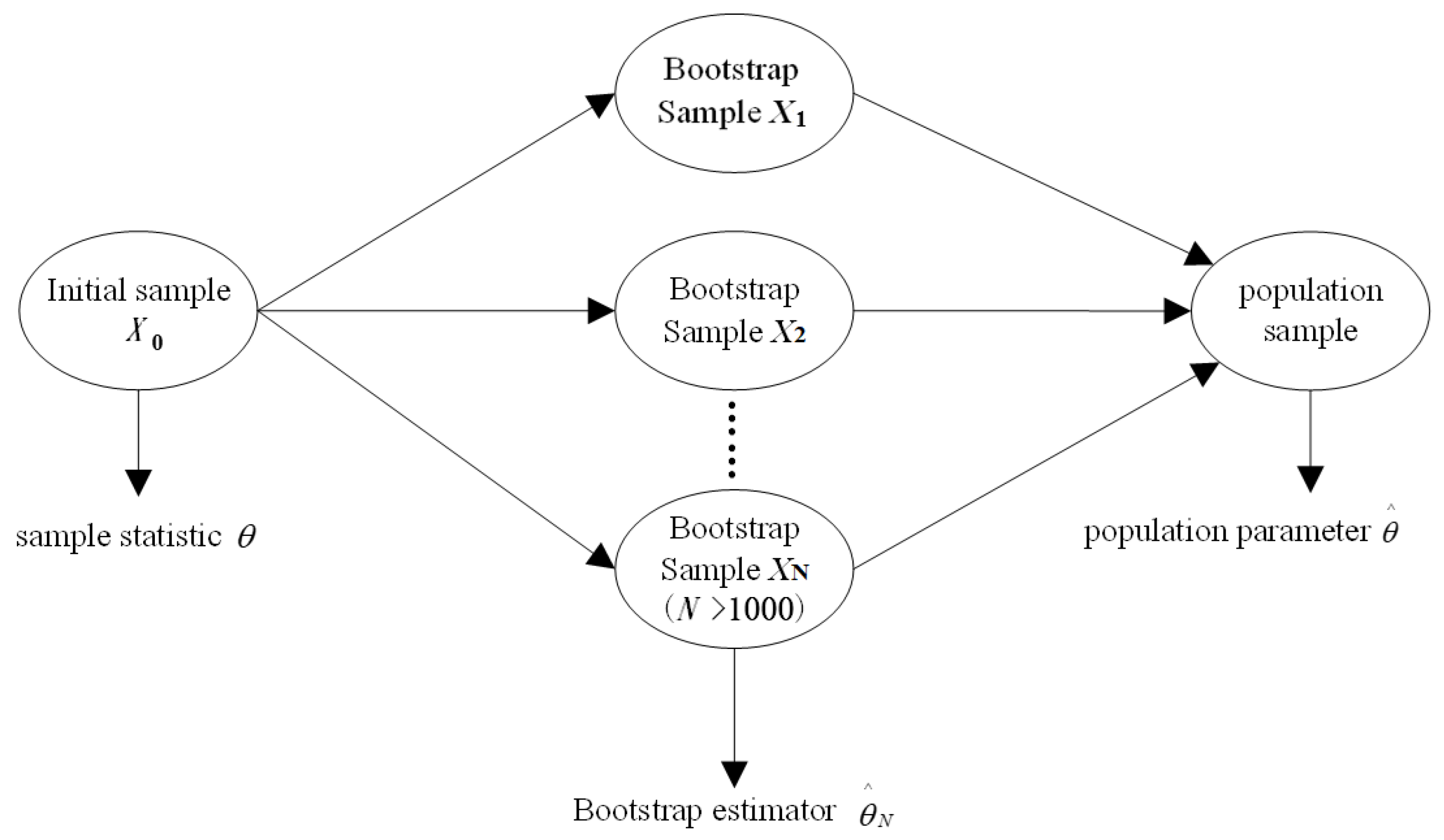
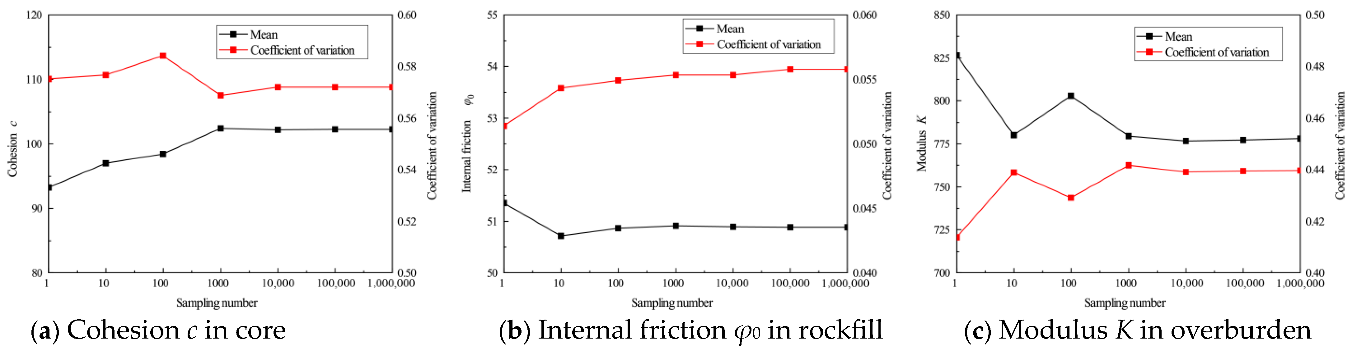
2.1.1. Material Parametric Statistical Method Based on Small-Sample Data

The nonparametric bootstrap sampling technique, proposed by Efron in 1979 [27], generates numerous bootstrap subsamples by selectively resampling the original limited data. This method allows for statistical analysis of small-sample data, offering a practical approach to overcoming sample size limitations.

Assuming (X₁, X₂, …, X_n) is the initial sample of geotechnical parameters, and the statistical parameters θ (mean, variance, etc.) of the sample are unknown, based on this sample, the target quantity θ is estimated as $\widehat{\theta }=\widehat{\theta }\hspace{0.33em}(X_1,X_2,\dots ,X_n)$. When the target quantity θ represents the mean of the sample, then $\widehat{\theta }={\displaystyle \frac{1}{n}}{\displaystyle \sum _{i=1}^n{X}_i}$. Due to the randomness of the sample, it is impossible to know the difference between the primary point estimation and the truth value of the parameter. The fluctuation of the point estimate can be obtained by multiple sampling techniques. While the overall distribution is unknown, an estimate of population distributions can be found to represent the population distributions. The essence of the bootstrap method is to replace the unknown population distribution with the empirical distribution. The bootstrap sampling method can produce new samples by sampling with replacement. Assuming a bootstrap sample $(X_1^{*},X_2^{*},\dots ,X_m^{*})$ is produced by random sampling from the initial sample (X₁, X₂,…, X_n), then the estimation $\widehat{\theta }$ based on the bootstrap sample is ${\widehat{\theta }}_m^{*}={\widehat{\theta }}_m(X_1^{*},X_2^{*},\dots ,X_m^{*})$. When applying repeated bootstrap sampling N times, then ${\widehat{\theta }}_{m1}^{*},{\widehat{\theta }}_{m2}^{*},\dots ,{\widehat{\theta }}_{mN}^{*}$ can be obtained. The point estimation and variance estimation of the overall sample based on the bootstrap method are shown in Equation (1), and the process of the bootstrap sample method is shown in Figure 1.

$$\left\{\begin{array}{l}{\widehat{\theta }}_{*}={\displaystyle \frac{1}{N}}{\displaystyle \sum _{i=1}^N{\hat{\theta }}_{n,i}^{*}}\\ v_N({\widehat{\theta }}^{*})={\displaystyle \frac{1}{N-1}}{\displaystyle \sum _{i=1}^N({\widehat{\theta }}_{n,i}^{*}}-{\widehat{\theta }}_n^{*}{)}^2\end{array}\right.$$

(1)

2.1.2. Marginal Distribution Test

The point estimation method commonly used in engineering has a limited capacity to evaluate the error between the estimated result and the true value, making it difficult to assess the reliability and accuracy of the estimate. In contrast, interval estimation not only determines the range within which parameters may lie but also provides the probability that the true parameters are contained within that range. During parameter interval estimation based on bootstrap sampling, N bootstrap samples were first generated to obtain parameter estimation values ${\widehat{\theta }}_i^{*}=\widehat{\theta }(x_1^{*i},x_2^{*i},\dots ,x_n^{*i},),i=1,2,\dots ,N$ of each sample, and then the parameters ${\widehat{\theta }}_1^{*},{\widehat{\theta }}_2^{*},\dots ,{\widehat{\theta }}_n^{*}$ were ranked from small to large [28].

The Kolmogorov–Smimov (K-S) and Anderson–Darling (A-D) tests can be used to estimate the marginal distribution of parameters. However, the results may vary depending on which test method is used, and some parameters may fit more than one distribution. As a result, the marginal distribution remains unclear for certain parameters. To address this, the Akaike information criterion (AIC) can be employed as a measure of the fitness of a statistical model. The AIC evaluates the goodness of fit based on the entropy principle [29,30], as shown in Equation (2),

$$AIC=-2{\displaystyle \sum _{i=1}^N\ln f(x_i;\epsilon )}+2k$$

(2)

where f (x_i; ε) is an alternative marginal distribution probability density function for the material parameter; x_i is the sample value of the material parameters to be tested; ε is the distribution parameter vector of the alternative marginal distribution probability density function; and k is the number of material parameters in the probability density function.

Based on the marginal distribution test, if a soil parameter fits multiple distribution types, the distribution with the smallest AIC value is considered the optimal fit for that parameter.

2.1.3. The Construction Method of a Multi-Dimensional Joint Distribution Model for Parameters

In the reliability analysis of rockfill dams, many studies have used a multi-dimensional normal distribution of random variables to establish the joint probability distribution function [31] or applied the Nataf transform to convert non-normal variables into independent variables. However, geotechnical parameters do not always follow a multi-dimensional normal distribution. Moreover, using a normal marginal distribution to describe the multi-dimensional probability distribution of random variables may underestimate the failure probability [32]. Thus, it is essential to develop a multi-dimensional joint probability distribution model to address the non-normal distribution of rockfill dam material parameters.

In the statistical analysis of rockfill dam material parameters, constructing the joint probability distribution function is challenging when material parameter distributions are non-normal. Copula theory offers a solution by allowing the establishment of a joint distribution function for non-normal distributions. Using Copula functions, a mathematical model can be developed that incorporates both the marginal distribution functions of the random parameters and the correlation functions between them.

Assume that X = {X₁, X₂,…, X_n} is an n-dimensional random vector and F_i(x_i) is the marginal distribution function of random variables; then, the joint distribution of random variables can be expressed by the Copula function as

$$F_X(x)=C(F_1(x_1),F_2(x_2),\dots ,F_n(x_n);\theta )$$

(3)

where X = {X₁, X₂,…, X_n} represents the random vectors; F_X(x) is the joint distribution function of random vectors; and θ is the correlation coefficient matrix of the Copula function.

Copula theory can be used to independently implement model construction including a marginal distribution of random parameters and correlation between parameters, thus avoiding the thorny problem of coupling modeling. There are many types of Copula functions that represent different correlation relationships between parameters. The Gaussian Copula, t Copula, Frank Copula, No. 16 Copula, and Clayton Copula can be used to express the symmetrical correlation between the random parameters. The Clayton Copula, Gumbel Copula, and Plackett Copula can be applied to represent the positive correlation between random parameters. Moreover, the t Copula, Clayton Copula, Clayton Copula, Gumbel Copula, and No. 16 Copula can represent the tail correlation between random parameters.

The multi-dimensional Gaussian Copula function and ellipse Copula function can describe the positive and negative correlations between parameters, and the correlation coefficient ranges from −1 to 1. These two Copula functions are widely used in ascertaining the uncertainty distribution of a multi-dimensional parameter field. So, these two Copula functions were used to construct the multi-dimensional joint probability density and distribution function of material parameters or constitutive model parameters of high core rockfill dams in this study.

The joint probability density function and distribution function of a multi-dimensional Gaussian Copula are as follows:

$$D(F_1(x_1),F_2(x_2),\dots ,F_n(x_n);\theta )=|\theta {|}^{-1/2}\exp [-{\displaystyle \frac{1}{2}}{\zeta }^{\prime }({\theta }^{-1}-I)\zeta ]$$

(4)

$$C(F_1(x_1),F_2(x_2),\dots ,F_n(x_n);\theta )={\mathsf{\Phi }}_n({\mathsf{\Phi }}^{-1}(F_1(x_1)),{\mathsf{\Phi }}^{-1}(F_2(x_2)),\dots ,{\mathsf{\Phi }}^{-1}(F_n(x_n));\theta )$$

(5)

where θ is the Copula correlation parameter matrix of n-dimensional random vectors; $|\theta |$ is the determinant of the correlation parameter; ${\zeta }^{\prime }=({\mathsf{\Phi }}^{-1}(u_1),{\mathsf{\Phi }}^{-1}(u_2),\dots ,{\mathsf{\Phi }}^{-1}(u_n))$ is the n-dimensional standard normal distribution variable; ${\mathsf{\Phi }}_n(•,\dots ,•;\theta )$ is the n-dimensional standard normal distribution function of the correlation parameter matrix θ; ${\mathsf{\Phi }}^{-1}(•)$ is the inverse function of the one-dimensional standard normal distribution; and I is the unit matrix.

The joint probability density function and distribution function of the multi-dimensional t Copula are as follows:

$$D(F_1(x_1),F_2(x_2),\dots ,F_n(x_n);\theta )=|\theta {|}^{-1/2}{\displaystyle \frac{\mathsf{\Gamma }(\frac{\nu +n}{2}){(\mathsf{\Gamma }(\frac{\nu }{2}))}^{n-1}}{{(\mathsf{\Gamma }(\frac{\nu +1}{2}))}^n}}{\displaystyle \frac{{(1+\frac{1}{\nu }{\zeta }^{\prime }{\theta }^{-1}\zeta )}^{\frac{\nu +n}{2}}}{{\displaystyle \prod _{i=1}^n{(1+\frac{{\zeta }_i^2}{\nu })}^{-\frac{\nu +1}{2}}}}}$$

(6)

$$C(F_1(x_1),F_2(x_2),\dots ,F_n(x_n);\theta )=T_n(T_{\nu }^{-1}(F_1(x_1)),T_{\nu }^{-1}(F_2(x_2)),\dots ,T_{\nu }^{-1}(F_n(x_n));\theta ,\nu )$$

(7)

where ${\zeta }^{\prime }=(T^{-1}(F_1(x_1)),T^{-1}(F_2(x_2)),\dots ,T^{-1}(F_n(x_n))$ is the t distribution variable with v degrees of freedom; $T_n(•,\dots ,•;\theta ,\nu )$ is the n-dimensional standard distribution function with correlation parameter matrix θ and v degrees of freedom; and ${T_v}^{-1}(•)$ is the inverse function of the one-dimensional t distribution of u_i with v degrees of freedom. The other symbols have the same meaning as before.

The elements θ of the correlation parameter matrix θ in the Copula function can be obtained by transforming Pearson correlation coefficients ρ as follows:

$$\rho ={\displaystyle {\int }_{-\propto }^{\propto }{\displaystyle {\int }_{-\propto }^{\propto }\dots {\displaystyle {\int }_{-\propto }^{\propto }\frac{x_1-{\mu }_1}{{\sigma }_1}\frac{x_2-{\mu }_2}{{\sigma }_2}\dots \frac{x_n-{\mu }_n}{{\sigma }_n}}}}D(F_1(x_1),F_2(x_2)\dots F_n(x_n);\theta )f_1(x_1)f_2(x_2)\dots f_n(x_n)d{x}_{1}d{x}_2\dots d{x}_n$$

(8)

The AIC can be used to judge which function can more reasonably describe the joint probability distribution of multiple parameters, shown as

$$AIC=-2{\displaystyle \sum _{i=1}^N\ln C\prime (F_1(x_1),F_2(x_2),\dots ,F_n(x_n);\theta )}+2k$$

(9)

where $C\prime (F_1(x_1),F_2(x_2),\dots ,F_n(x_n);\theta )$ is the maximum likelihood function value of the Copula distribution function; k is the number of correlation parameters in the Copula function; and $F_1(x_1),F_2(x_2),\dots ,F_n(x_n)$ is the marginal distribution of material parameters or constitutive model parameters of rockfill dams.

2.2. Cracking Risk Analysis Method for the Core Wall

Uneven deformation of the core wall may result from variations in soil compressibility across different sections, as well as factors such as water immersion and creep deformation during operation. The extent of uneven deformation and the potential for soil cracking are typically assessed by evaluating the degree of deformation inclination. Thus, the cracking of the core wall due to uneven deformation can be judged by checking whether the deformation inclination at various positions exceeds the empirical allowable value [33], that is,

$$f(\delta )={\delta }_0-\delta$$

(10)

where δ₀ is the allowable value of deformation inclination, and δ is the calculation value of deformation inclination.

Usually, the surrogate model can be used to reduce the difficulty of solving the above performance function (Equation (10)). Here, a quadratic response surface method without considering the cross term is introduced as a surrogate model, which can be computed as

$${\sigma }_t=a_0+{\displaystyle \sum _{i=1}^n{b}_i{X}_i+{\displaystyle \sum _{i=1}^n{c}_i{X}_i^2}}$$

(11)

where σ_t are stress calculation values of characteristic points, X_i is the random variable and a₀, b_i, and c_i are parameters of the response surface equation to be solved.

Based on Equation (11), Combined with the multi-dimensional joint distribution model, the Monte Carlo method [34] is adopted and sample values of X = {x₁, x₂,…, x_n }^T are selected as the random samples. Additionally, an extra function with values of 0 and 1 is constructed:

$$I\left[G\left(x\right)\right]=\left\{\begin{array}{c}1, \hspace{0.17em}G\left(x\right)<0,\hspace{0.33em}Cracking\\ 0, G\left(x\right)\ge 0,\hspace{0.33em}\hspace{0.33em}\hspace{0.33em}\hspace{0.33em}\hspace{0.33em}\hspace{0.33em}Safety\end{array}\right.$$

(12)

where I[·] is the function symbol; and G(x) is the value of the performance function G(X).

Then, the sampling estimation of failure probability ${\widehat{P}}_f$ can be obtained as

$${\widehat{P}}_f={\displaystyle \frac{1}{N}}{\displaystyle \sum _{i=1}^{N}I\left[G{\left(x\right)}_i\right]}$$

(13)

where N is the total sampling number; G(x)_i is the value of the performance function corresponding to the ith sampling; and other symbols have the same meaning as before.

3. Case Study

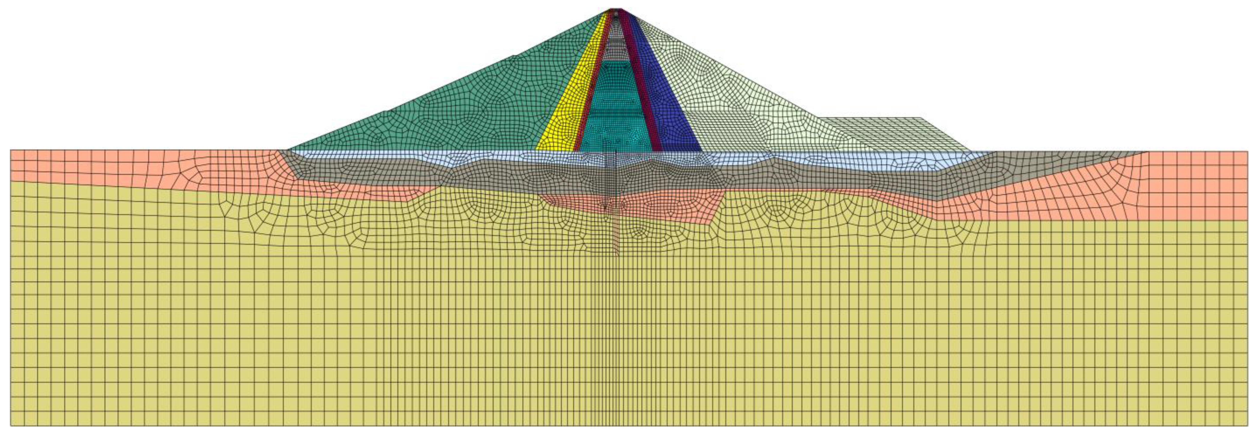
3.1. Project Specification

A high core rockfill dam, named PB, was selected as the case study to verify the feasibility and effectiveness of the proposed method, and a typical cross-section is shown in Figure 2. It is noted that the overburden of the dam foundation can be divided into four layers: the floated boulder and pebble layer (${\mathrm{Q}}_3^2$), the pebble and gravel layer (${\mathrm{Q}}_4^{\text{1-1}}$), the pebble layer with boulders (${\mathrm{Q}}_4^{\text{1-2}}$), and the boulder and pebble layer (${\mathrm{Q}}_4^2$). To study the effects of independent and joint sampling of material parameters on the stress and deformation of high core rockfill dams, a generalized plane model referring to the PB Hydropower Station was constructed, and the size information for the conceptual model of a high core rockfill dam was as follows: the dam height was 200 m, the water depth in front of the dam was 190 m, the crest width was 14 m, and the upstream and downstream slope ratio was 1:0.25. The dam body included upstream and downstream rockfill areas, transition layers, inverted flayers, and a core wall. The foundation included the overburden (thickness: 70 m) and the bedrock.

The dam–foundation system was discretized into 4798 nodes and 2335 elements (see Figure 3). The X axis pointed downstream, while the Y axis extended upward. The upstream and downstream boundaries of the model were controlled by normal displacement methods, and the bottom boundary was constrained rigidly.

3.2. Statistical Analysis of the Multi-Dimensional Joint Distribution Model for the Duncan–Chang Model Parameters

3.2.1. Interval Estimation of the Duncan–Chang Model Parameters for High Rockfill Dams

The Duncan–Chang E-B model is a widely used soil constitutive model in the numerical simulation of stress and deformation in earth–rock dams. This nonlinear elastic model accounts for the nonlinear characteristics of soil material deformation and uses a hyperbola to fit the triaxial test data.

A total of 155 groups of parameter test data for the Duncan–Chang E-B model were collected from several high core rockfill dams and dam foundation overburdens. The material parameter samples included 52 groups for the core wall, 59 groups for the rockfill, and 44 groups for the overburden. The core of the bootstrap sampling method involves randomly sampling the original experimental data with replacement to generate numerous subsamples of the same size as the original data. By repeatedly sampling and estimating, a series of statistical values are obtained, from which confidence intervals and probability distributions can be derived to assess the variability of these values. To determine the optimal sampling frequency for the bootstrap method, sampling tests with different frequencies were conducted. Figure 4 shows the relationship curves between the mean value and the coefficient of variation of the cohesion c of the core wall, the internal friction angle of the rockfill material, and the deformation modulus K of the overburden and the bootstrap sampling frequency. As can be seen from Figure 4, when the sampling frequency exceeds 10,000, the mean value and coefficient of variation of parameters c and K are stable. Therefore, a sampling frequency of 10,000 was adopted for the bootstrap method in the subsequent research.

Based on the statistical characteristic values of the Duncan–Chang E-B model parameters for the core material, rockfill material, and dam foundation overburden of the high core rockfill dam, the interval estimation with a 95% confidence level is presented in

Table 1. Interval estimation of the Duncan–Chang E-B model parameters in the core wall.

Parameter		c/kPa	φ/°	Rf	K	Kb	m	n
Mean	Lower limit	89.65	26.48	0.81	407.00	291.06	0.29	0.42
	Upper limit	115.92	28.20	0.83	442.02	328.05	0.35	0.47
SD	Lower limit	50.62	3.43	0.05	65.18	70.67	0.11	0.10
	Upper limit	64.71	4.38	0.07	98.45	94.33	0.14	0.14
VC	Lower limit	0.51	0.12	0.06	0.15	0.23	0.34	0.21
	Upper limit	0.63	0.16	0.08	0.22	0.30	0.44	0.32

Note: SD, standard deviation; VC, variation coefficient.

,

Table 2. Interval estimation of the Duncan–Chang E-B model parameters in the rockfill.

Parameter		${\mathit{\phi }}_0\mathbf{/}\mathbf{°}$	$\mathbf{\Delta }\mathit{\phi }\mathbf{/}\mathbf{°}$	Rf	K	Kb	m	n
Mean	Lower limit	50.31	8.18	0.74	1013.69	500.12	0.24	0.27
	Upper limit	51.47	8.97	0.77	1131.78	570.88	0.28	0.30
SD	Lower limit	2.25	1.57	0.07	256.02	142.96	0.09	0.07
	Upper limit	3.39	2.25	0.08	336.70	196.82	0.13	0.10
VC	Lower limit	0.04	0.18	0.09	0.22	0.26	0.35	0.25
	Upper limit	0.06	0.26	0.11	0.31	0.37	0.47	0.33

Note: SD, standard deviation; VC, variation coefficient.

and

Table 3. Interval estimation of the Duncan–Chang E-B model parameters in the overburden.

Parameter		${\mathit{\phi }}_0/°$	Rf	K	Kb	m	n
Mean	Lower limit	38.38	0.78	699.54	332.01	0.25	0.41
	Upper limit	41.21	0.81	858.70	405.55	0.30	0.44
SD	Lower limit	5.27	0.06	302.52	137.58	0.08	0.05
	Upper limit	6.99	0.08	381.92	186.23	0.12	0.08
VC	Lower limit	0.13	0.07	0.37	0.36	0.31	0.13
	Upper limit	0.17	0.10	0.51	0.51	0.42	0.19

Note: SD, standard deviation; VC, variation coefficient.

. The results show that the parameters with the highest interval estimation values of the coefficient of variation for the core wall, rockfill, and overburden are the cohesion, the exponent of the volume modulus, and the volume variation modulus, respectively. Among these, the coefficient of variation for the cohesion c of the core wall is the highest, ranging from 0.51 to 0.63. The mean of R_f of the core wall is the highest, followed by the overburden and rockfill materials, with the variation coefficients of the failure ratios for all three materials being relatively small. The variation coefficients of K and K_b are similar across the three materials. Notably, the variation coefficient of the deformation modulus of the overburden is the highest, while those of the core wall and rockfill materials are comparable. This may be due to the core wall and rockfill materials being manually compacted, resulting in controlled physical and mechanical properties (e.g., dry density) and less modulus anisotropy compared to the natural overburden. Additionally, the variation coefficients of the exponent of the volume modulus are the same for the three materials. The variation coefficient of the exponent of the initial deformation modulus is smallest in the overburden and identical in the core wall and rockfill.

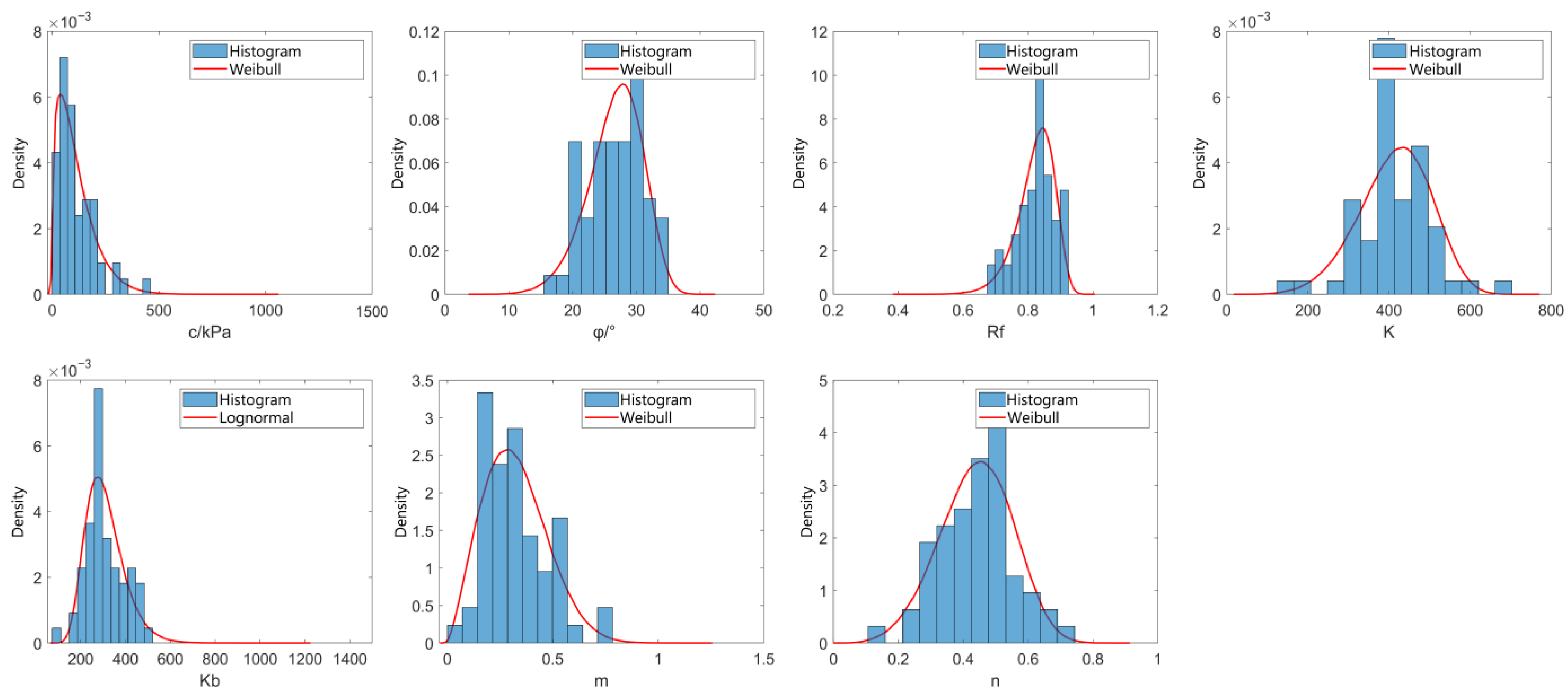
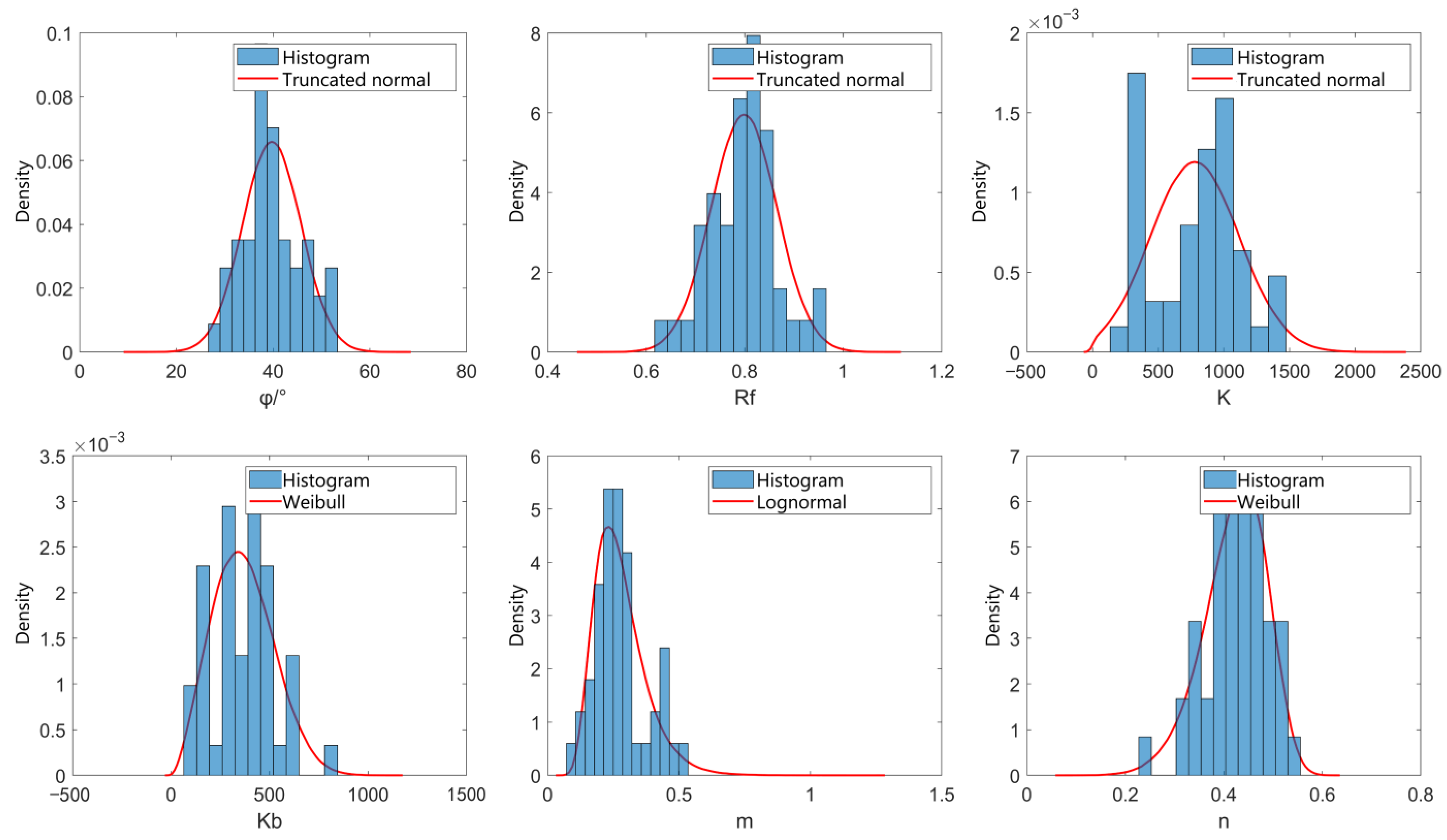
3.2.2. Distribution Types of the Duncan–Chang Model Parameters

Based on the test data samples of high core rockfill dams and foundation material parameters, the K-S and A-D test methods were used to evaluate the marginal distribution types of the Duncan–Chang E-B model parameters. The results are shown in

Table 4. The marginal distribution of the Duncan–Chang model in the core wall.

Parameters	K-S Test				A-D Test
	Truncated Normal Distribution	Lognormal Distribution	Extremal Distribution	Weibull Distribution	Truncated Normal Distribution	Lognormal Distribution	Extremal Distribution	Weibull Distribution
c/kPa	✗	✓	✗	✓	✗	✓	✗	✓
φ/°	✓	✗	✓	✓	✓	✗	✓	✓
Rf	✗	✗	✓	✓	✗	✗	✓	✓
Kb	✓	✗	✗	✓	✓	✗	✗	✗
m	✗	✓	✗	✗	✗	✓	✗	✗
n	✗	✗	✗	✓	✗	✗	✗	✓
Rf	✓	✗	✗	✓	✓	✗	✗	✓

,

Table 5. The marginal distribution of the Duncan–Chang model in the rockfill.

Parameters	K-S Test				A-D Test
	Truncated Normal Distribution	Lognormal Distribution	Extremal Distribution	Weibull Distribution	Truncated Normal Distribution	Lognormal Distribution	Extremal Distribution	Weibull Distribution
c/kPa	✗	✗	✗	✓	✓	✗	✗	✓
φ/°	✓	✗	✓	✓	✗	✗	✓	✓
Rf	✓	✓	✗	✗	✓	✓	✗	✗
Kb	✓	✗	✗	✓	✓	✓	✗	✗
m	✓	✗	✗	✓	✓	✗	✗	✓
n	✓	✗	✗	✓	✓	✓	✗	✓
Rf	✗	✓	✗	✗	✗	✓	✗	✗

and

Table 6. The marginal distribution of the Duncan–Chang model in the overburden.

Parameters	K-S Test				A-D Test
	Truncated Normal Distribution	Lognormal Distribution	Extremal Distribution	Weibull Distribution	Truncated Normal Distribution	Lognormal Distribution	Extremal Distribution	Weibull Distribution
$\phi /°$	✓	✓	✗	✗	✓	✓	✗	✗
$R_f$	✓	✓	✗	✗	✓	✓	✗	✗
$K$	✓	✗	✓	✗	✗	✗	✗	✗
$K_b$	✓	✗	✓	✓	✓	✗	✓	✓
$m$	✗	✓	✗	✗	✗	✓	✗	✗
$n$	✓	✓	✓	✓	✓	✓	✓	✓

, in which ✓ indicates that the parameter follows a distribution form, and ✗ indicates that the parameter does not follow a distribution form. The marginal distribution is not always consistent across the K-S and A-D test methods, and some parameters may conform to more than one distribution. As a result, the marginal distribution remains unclear for some parameters. To address this, the Akaike information criterion (AIC) was employed in this study.

Here, the result with the minimum AIC value is the optimal marginal distribution, as shown in

Table 7. The optimal marginal distribution of the Duncan–Chang model in the core wall.

Parameters	AIC				Optimal Marginal Distribution
	Truncated Normal Distribution	Lognormal Distribution	Extremal Distribution	Weibull Distribution
c/kPa	/	731.14	/	709.16	Weibull distribution
φ/°	376.34	/	528.79	359.73	Weibull distribution
Rf	/	/	−133.27	−184.43	Weibull distribution
K	744.71	/	/	730.80	Weibull distribution
Kb	/	/	/	/	Lognormal distribution
m	/	/	/	/	Weibull distribution
n	−85.36	/	/	−100.70	Weibull distribution

,

Table 8. The optimal marginal distribution of the Duncan–Chang model in the rockfill.

Parameters	AIC				Optimal Marginal Distribution
	Truncated Normal Distribution	Lognormal Distribution	Extremal Distribution	Weibull Distribution
φ0/°	388.22	/	/	490.91	Truncated normal distribution
$\Delta \phi$/°	478.74	/	595.76	457.02	Weibull distribution
Rf	−185.30	−187.36	/	/	Lognormal distribution
K	1125.10	1126.40	/	1105.90	Weibull distribution
Kb	1032.50	/	/	1008.60	Weibull distribution
m	−123.15	−100.23	/	−159.68	Weibull distribution
n	/	/	/	/	Lognormal distribution

and

Table 9. The optimal marginal distribution of the Duncan–Chang model in the overburden.

Parameters	AIC				Optimal Marginal Distribution
	Truncated Normal Distribution	Lognormal Distribution	Extremal Distribution	Weibull Distribution
φ/°	546.37	569.27	/	/	Truncated normal distribution
Rf	−156.37	−153.66	/	/	Truncated normal distribution
K	1133.80	/	1145.10	/	Truncated normal distribution
Kb	1065.70	/	1049.10	1009.90	Weibull distribution
m	/	/	/	/	Lognormal distribution
n	−72.56	−77.49	−76.99	−103.41	Weibull distribution

. The parameters in the core wall obey a Weibull distribution, except K_b, which obeys a lognormal distribution. The internal friction angle φ₀ in the rockfill follows a truncated normal distribution, R_f and n obey a lognormal distribution, and the other parameters follow a Weibull distribution. The parameter m in the overburden obeys a lognormal distribution, K_b and n follow a Weibull distribution, and other parameters obey a truncated normal distribution.

Based on the above results, this study employed the bootstrap sampling method to generate 10,000 groups of parameter subsamples for the Duncan–Chang E-B model to verify whether the distribution features of statistical data were reasonable by analyzing the variability of statistical eigenvalues of the subsamples. The results of our efforts at generating subsamples for each parameter and testing their marginal distribution are presented in

Table 10. The marginal distribution of the Duncan–Chang model in the core wall based on the bootstrap method.

Marginal Distribution	c/kPa	φ/°	Rf	K	Kb	m	n
Truncated normal distribution	40	0	172	37	0	0	0
Lognormal distribution	375	5	15	213	9932	0	61
Extremal distribution	2016	1	0	116	56	0	2
Weibull distribution	7569	9994	9813	9634	12	10,000	9937

,

Table 11. The marginal distribution of the Duncan–Chang model in the rockfill based on the bootstrap method.

Marginal Distribution	φ0/°	Δφ/°	Rf	K	Kb	m	n
Truncated normal distribution	9711	34	259	0	0	0	0
Lognormal distribution	0	0	6777	32	2	0	8183
Extremal distribution	0	0	2531	80	6	0	602
Weibull distribution	289	9966	433	9888	9992	10,000	1215

and

Table 12. The marginal distribution of the Duncan–Chang model in the overburden based on the bootstrap method.

Marginal Distribution	φ/°	Rf	K	Kb	m	n
Truncated normal distribution	8298	9336	10,000	0	0	0
Lognormal distribution	79	419	0	0	9939	0
Extremal distribution	2	5	0	0	6	0
Weibull distribution	1621	240	0	10,000	55	10,000

. As can be seen in these tables, the marginal distribution test results for the bootstrap subsample of the high core rockfill dam material are consistent with the statistical sample test results, thereby verifying the correctness of the marginal distribution test results for the material parameters.

Figure 5, Figure 6 and Figure 7 show the marginal distribution probability density curves and histograms of the Duncan–Chang E-B model parameters of samples for the core wall material, rockfill, and dam foundation overburden, respectively. Here, the marginal distribution probability density curves closely match the probability distribution of the sample parameters.

3.2.3. The Multi-Dimensional Joint Distribution Model for the Duncan–Chang Model Parameters

Correlation Analysis of Duncan–Chang Model Parameters

Many geotechnical tests have shown that the mechanical parameters of geotechnical materials are not mutually independent but exhibit a certain degree of correlation. Based on the parameter test data, the Pearson correlation coefficients (PCCs) between the Duncan–Chang E-B model parameters are given in

Table 13. The correlation coefficient among the parameters in the Duncan–Chang E-B model in the core wall.

Parameters	c/kPa	φ/°	Rf	K	Kb	m	n
$c/kPa$	1.00	−0.68	0.31	0.15	0.17	−0.31	0.06
$\phi /°$		1.00	0.12	0.34	0.22	−0.35	0.28
$R_f$			1.00	0.53	0.07	0.41	−0.08
$K$				1.00	0.63	0.41	0.02
$K_b$					1.00	0.11	0.18
$m$						1.00	0.40
$n$							1.00

,

Table 14. The correlation coefficient among the parameters in the Duncan–Chang E-B model in the rockfill.

Parameters	φ0/°	Δφ/°	Rf	K	Kb	m	n
${\phi }_0/°$	1.00	0.78	0.41	0.37	0.34	0.04	0.28
$\Delta \phi /°$		1.00	0.43	0.39	0.26	−0.09	0.01
$R_f$			1.00	0.25	0.15	0.28	0.05
$K$				1.00	0.74	−0.01	−0.04
$K_b$					1.00	−0.17	0.23
$m$						1.00	0.60
$n$							1.00

and

Table 15. The correlation coefficient among the parameters in the Duncan–Chang E-B model in the overburden.

Parameters	φ/°	Rf	K	Kb	m	n
$\phi /°$	1.00	0.03	0.57	0.40	0.19	−0.21
$R_f$		1.00	0.20	0.27	0.06	0.21
$K$			1.00	0.87	0.11	−0.17
$K_b$				1.00	0.08	0.06
$m$					1.00	0.14
$n$						1.00

. The results show that the correlation coefficients of c~φ and K~K_b in the core wall, as well as those of φ₀~Δφ and K~K_b in the rockfill, all range between 0.6 and 0.8, indicating a strong correlation. Additionally, the correlation coefficient of K~K_b in the overburden is 0.87, indicating an extremely strong correlation.

In total, 10,000 groups of samples were generated using the bootstrap sampling method. Aside from the strong correlations for c~φ and K~K_b in the core wall, the bootstrap sampling analysis results indicated that 57.87% of the samples for m~n had strong correlations, which meant that the strong correlation for m~n would be neglected with traditional small-sample processing methods. Similarly, there was also a strong correlation for m~n in the overburden. However, the strong correlation for m~n in the rockfill was only supported by 20% of the sample data. Therefore, parameters that can be considered to have a strong correlation include c~φ, K~K_b, and m~n in the core wall, φ₀~Δφ and K~K_b in the rockfill, and K~K_b and m~ n in the overburden.

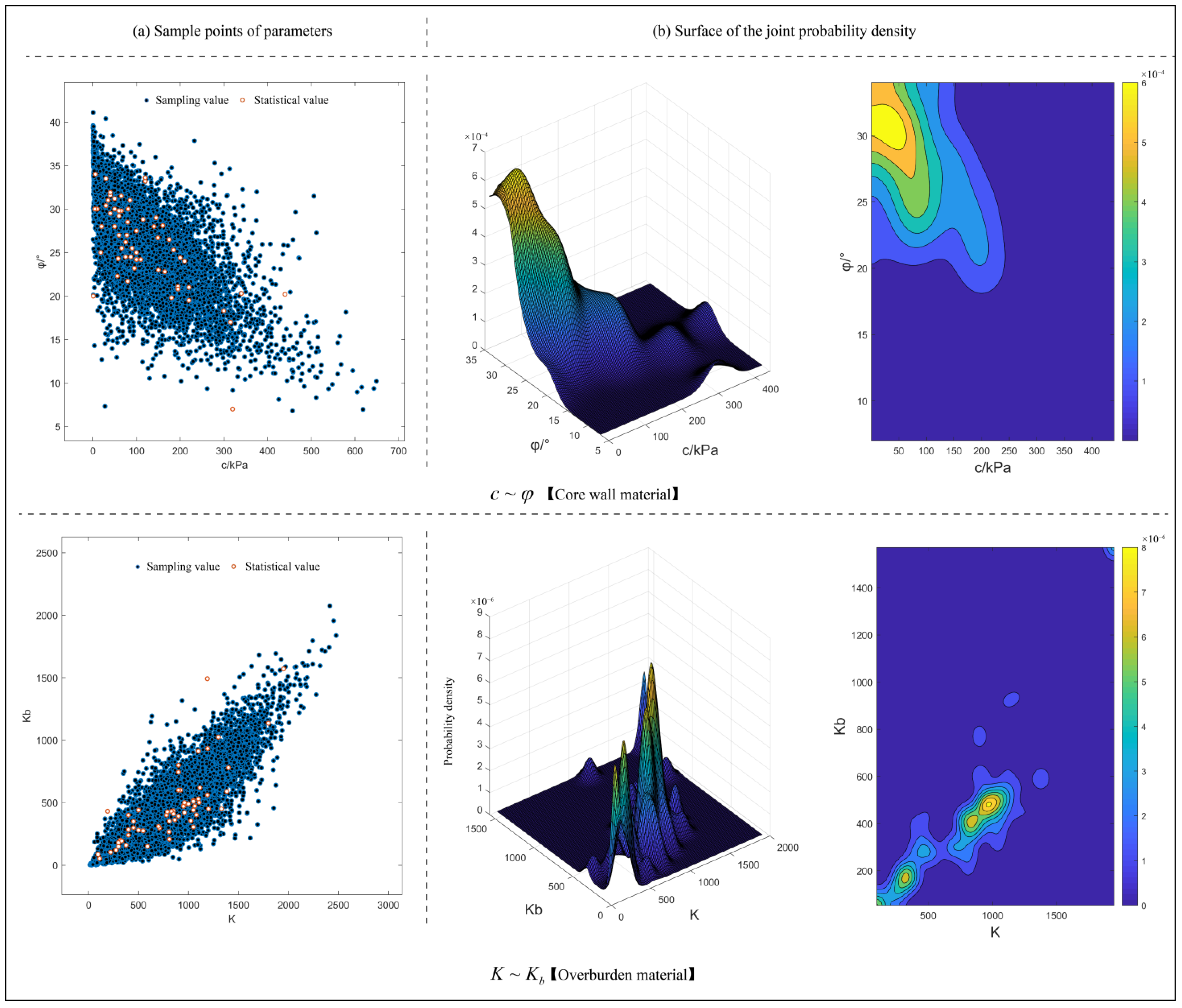
Construction of the Multi-Dimensional Joint Distribution Model for the Duncan–Chang Model Parameters

Based on Equations (4)–(8) and the marginal distribution types of Duncan–Chang model parameters, the corresponding multi-dimensional joint probability density functions and distribution functions could be constructed using the Gaussian Copula and t Copula as follows:

$$\left\{\begin{array}{l}D(c,\phi ,R_f,K,K_b,m,n;\theta )=|\theta {|}^{-1/2}\exp [-{\displaystyle \frac{1}{2}}{\zeta }^{\prime }({\theta }^{-1}-I)\zeta ]\\ C(c,\phi ,R_f,K,K_b,m,n;\theta )={\mathsf{\Phi }}_n({\mathsf{\Phi }}^{-1}(c),{\mathsf{\Phi }}^{-1}(\phi ),\dots ,{\mathsf{\Phi }}^{-1}(n);\theta )\end{array}\right.$$

(14)

$$\left\{\begin{array}{l}D(c,\phi ,R_f,K,K_b,m,n;\theta )=|\theta {|}^{-1/2}{\displaystyle \frac{\mathsf{\Gamma }(\frac{\nu +n}{2}){(\mathsf{\Gamma }(\frac{\nu }{2}))}^{n-1}}{{(\mathsf{\Gamma }(\frac{\nu +1}{2}))}^n}}{\displaystyle \frac{{(1+\frac{1}{\nu }{\zeta }^{\prime }{\theta }^{-1}\zeta )}^{\frac{\nu +n}{2}}}{{\displaystyle \prod _{i=1}^n{(1+\frac{{\zeta }_i^2}{\nu })}^{-\frac{\nu +1}{2}}}}}\\ C(c,\phi ,R_f,K,K_b,m,n;\theta )=T_n\left(T^{-1}(c),T^{-1}(\phi ),\dots ,T^{-1}(n),\theta ,\nu \right)\end{array}\right.$$

(15)

where c, φ, R_f, K, K_b, m, and n are the Duncan–Chang model parameters in the high core rockfill dams.

To verify the applicability of the two functions, 10,000 sample sets were analyzed, and the test results for the multi-dimensional joint probability model of Duncan–Chang model parameters are presented in

Table 16. Test results of the Copula function based on the AIC.

Materials	AIC		Number of t Copula < Gaussian Copula
	Gaussian Copula	t Copula
Core wall	−139.95	−164.10	6720
Rockfill	−251.10	−264.43	8333
Overburden	−137.02	−171.37	6282

. As shown in Table 16, the t Copula function performs better in describing the multi-dimensional joint probability distribution of Duncan–Chang E-B model parameters for core wall, rockfill, and dam foundation overburden materials. Additionally, the parametric samples effectively cover the original samples (see Figure 8), indicating that the multi-dimensional joint distribution model for Duncan–Chang model parameters based on the t Copula function can accurately capture the nonlinear correlations between parameters and their joint probability distribution.

Based on the statistical analysis of Duncan–Chang model parameters, the random characteristics of parameters in the dam and foundation are shown in

Table 17. Random characteristics of parameters in the dam and foundation (1).

		c	Internal Friction Angle			Rf	K	Kb	m	n
			φ	φ0	Δφ
Core wall	Mean	0.06(MPa)	35°	/		0.68	411.0	185.0	0.30	0.68
	VC	0.57	0.14			0.07	0.19	0.27	0.39	0.27
	Type	Weibull	Weibull			Weibull	Weibull	Lognormal	Weibull	Weibull
Main rockfill	Mean	/	/	30.76	10.0	0.63	1184.0	489.0	0.33	0.35
	VC	/	/	0.05	0.22	0.10	0.27	0.32	0.41	0.29
	Type	/	/	Truncated normal	Weibull	Lognormal	Weibull	Weibull	Weibull	Lognormal
Secondary rockfill	Mean	/	/	28.6	8.3	0.64	1027.0	380.0	0.36	0.36
	VC	/	/	0.05	0.22	0.10	0.27	0.32	0.41	0.29
	Type	/	/	Truncated normal	Weibull	Lognormal	Weibull	Weibull	Weibull	Lognormal
Overburden	Mean	/	38°	/		0.64	780.0	400.0	0.18	0.42
	VC	/	0.15			0.09	0.44	0.44	0.37	0.16
	Type	/	Truncated normal			Truncated normal	Truncated normal	Weibull	Lognormal	Weibull

and

Table 18. Random characteristics of parameters in the dam and foundation (2).

		Mean	VC	Type
Cutoff Wall	c (MPa)	1.13	0.25	Lognormal
	φ (°)	42.3	0.15	Normal
	E (GPa)	28.5	0.10	Lognormal
Bedrock	c (MPa)	1.30	0.30	Lognormal
	φ (°)	49.0	0.20	Normal
	E (GPa)	9.0	0.15	Lognormal

, and the multi-dimensional joint probability density functions of Duncan–Chang model parameters can be described by Equation (15).

3.3. Cracking Risk Analysis of the Core Wall

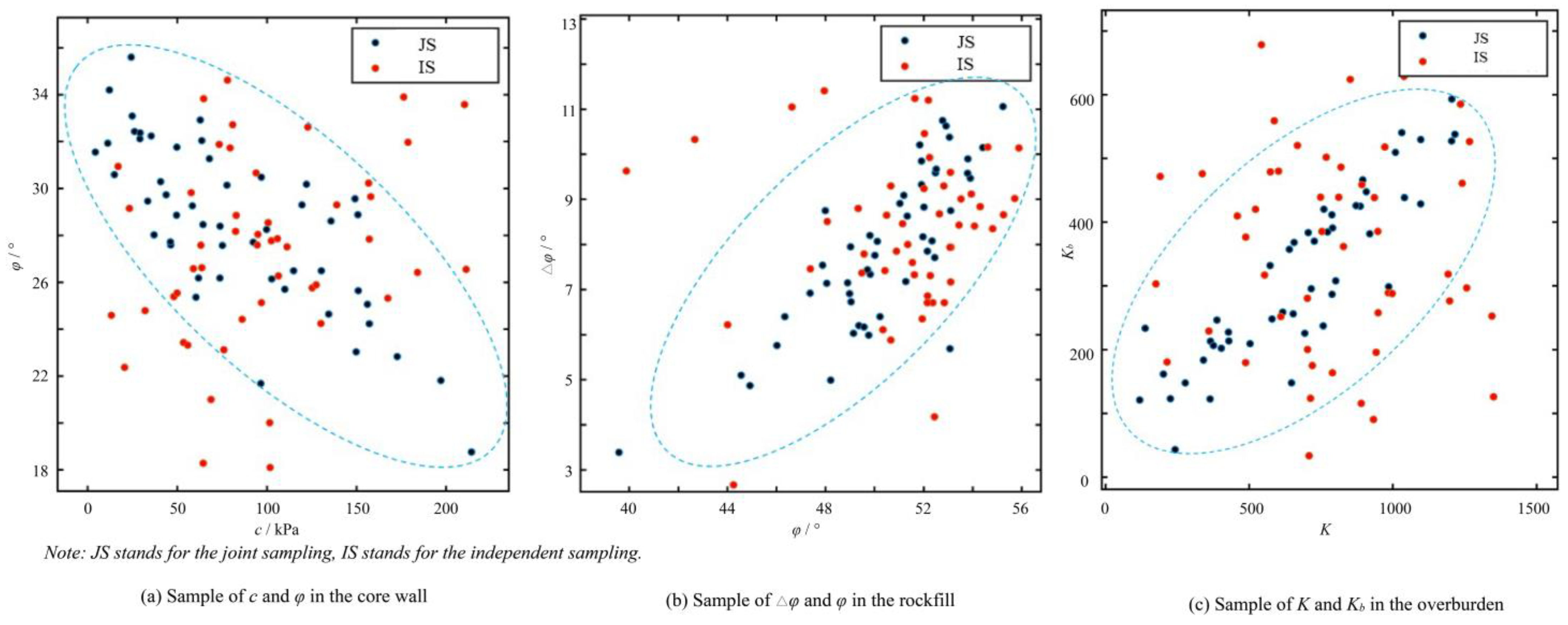
3.3.1. Analysis of the Sample Point Change Law for Independent and Joint Sampling of Parameters

Through the independent (IS) and joint sampling (JS) of the Duncan–Chang model parameters, a sample scatter plot was compiled, as shown in Figure 9. For the method of independent sampling, the sample points of each parameter are random, without any associated features, and do not conform to the true law of material parameters, such as the negative correlation for c~φ in the core wall, the positive correlation for φ₀~Δφ in the rockfill, etc. For the method of joint sampling, the sample points of each parameter exhibit good correlation characteristics, which conform to the inherent correlation law of material mechanical parameters. For example, c~φ of the core wall, φ₀~Δφ of the rockfill, and K~K_b of the overburden all exhibit correlation laws that are consistent with their statistical characteristics. This implies that in the safety risk analysis of high core rockfill dams, if the relevant laws of material parameters are not considered, it will cause physical distortion in parametric sampling and form unreasonable evaluation results.

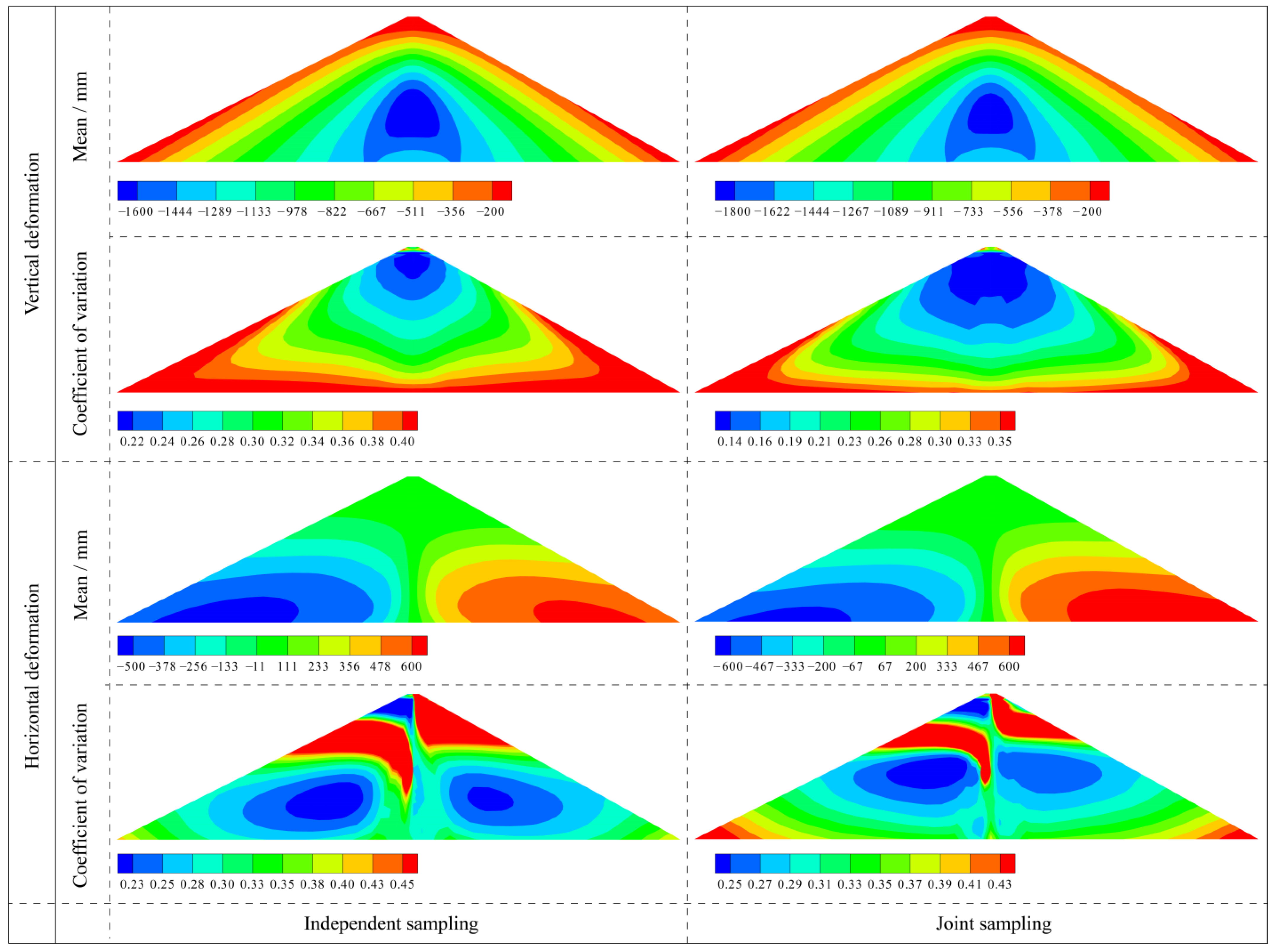
3.3.2. Analysis of the Deformation and Stress of Dams Based on the Independent and Joint Sampling of Parameters

Based on the statistical characteristics and distribution types of material parameters in Table 17, 300 sets of samples were generated using both independent and joint sampling methods for finite element simulation. The resulting mean and coefficient of variation cloud maps for deformation, principal stress, and the stress level are shown in Figure 10 and Figure 11. As depicted in Figure 10 and Figure 11, the means of the major and minor principal stresses are only slightly affected by the sampling method, with a maximum difference of 1.8%. However, the mean stress level is significantly influenced, showing an 8.7% increase when using the joint sampling method. Additionally, the means of vertical and horizontal deformations are higher with the joint sampling method compared to the independent sampling method, with increases of 12.5% and 8.7%, respectively.

Compared to the results obtained using the independent sampling method, the coefficients of variation for dam deformation and stress using the joint sampling method are relatively smaller. Specifically, the coefficient of variation for major and minor principal stresses and stress levels are reduced by 27.9%, 10.1%, and 21.0%, respectively. Additionally, the coefficient of variation for vertical and horizontal deformations is reduced by 12.5% and 4.6%, respectively.

3.3.3. Analysis of the Cracking Risk

Since the densities of concrete, the foundation, fractures, and disturbed zones vary little, 30 random parameters were identified, including the reservoir water level, Duncan–Chang E-B model parameters for the core wall, rockfill, and overburden materials, as well as cohesion, the friction angle, and the elastic moduli of the cutoff wall, galleries, and curtain materials. Based on Equation (11), the response surface equation for the performance function related to core wall cracking was established as follows:

$$G(X)={\displaystyle \sum _{i=1}^n{b}_i}{X_i}^2+{\displaystyle \sum _{i=1}^n{c}_i}{X}_i+a_0=A{X_1}^{\mathrm{T}}$$

(16)

$$X_1=[1,x_1,x_2,\dots ,x_{29},x_{30},x_1^2,x_2^2,\dots x_{29}^2,{x^2}_{30}]$$

(17)

where X₁ is the random variable matrix, and x₁, x₂, …, and x₃₀ are the random variables for analyzing the cracking risk of the core wall.

Using the response surface equation for the performance function related to core wall cracking in the PB dam, Monte Carlo simulation, the proposed stochastic characteristics, and a joint distribution model for multi-component material parameters of high core rockfill dams were employed. The number of sampling iterations significantly affects the risk probability results. Since the risk probability P_f of the dam failure in Equation (13) is usually very small (e.g., less than 0.001), it is recommended that the number of samples N satisfies N ≥ 100/P_f [35]. Consequently, the cracking risk of the core wall was determined to be 2.14 × 10⁻⁷ using the Monte Carlo simulation.

4. Conclusions

An interval estimation of the statistical parameters of the Duncan–Chang E-B model for high core rockfill dam materials is proposed. The bootstrap method was used to estimate the mean value, standard deviation, and coefficient of variation for the Duncan–Chang E-B model parameters of the core wall, rockfill, and overburden based on 155 groups of test data. The maximum and minimum variation coefficients of the parameters are as follows: the cohesion c and the failure ratio R_f in the core wall, the exponent of the volume modulus m and the internal friction angle φ in the rockfill, and the exponent of the volume modulus m and the failure ratio R_f in the overburden. The mean value of the internal friction angle φ in the core wall material is the smallest, while the mean value of the internal friction angle φ₀ in the rockfill material is the largest, with the minimum variation coefficient, while the variation coefficient of Δφ is large.

The marginal distribution types of Duncan–Chang E-B model parameters for high core rockfill dam materials are proposed. Since the marginal distribution is not always consistent when using the K-S and A-D test methods, AIC optimization is employed to accurately estimate the marginal distribution types of these parameters. In addition to K_b of the core wall material following a lognormal distribution, the other parameters of the core wall follow a Weibull distribution. The internal friction angle φ₀ of the rockfill follows a truncated normal distribution, Δφ, K, K_b, and m follow a Weibull distribution, and the other parameters of the rockfill follow a lognormal distribution. φ, R_f, and K of the overburden obey a truncated normal distribution, m obeys a lognormal distribution, and the other parameters obey a Weibull distribution. Furthermore, the results obtained through bootstrap sampling are consistent with those from the statistical sample tests.

Based on the correlation analysis and marginal distribution results of the Duncan–Chang model parameters, a multi-dimensional joint distribution model for the parameters of the core wall, rockfill, and overburden materials in high core rockfill dams was established using the t Copula function. The samples generated by this method demonstrate that the correlation laws effectively represent the original samples and reasonably describe the correlation and joint probability distribution of the Duncan–Chang E-B model parameters for high core rockfill dam materials.

A method for analyzing the cracking risk of the core wall using the multi-dimensional joint distribution of Duncan–Chang model parameters is proposed, leading to a more reasonable security assessment. The results for the PB dam demonstrate that joint sampling effectively captures the internal correlation between material mechanical parameters. In contrast, independent sampling can introduce physical distortions in parametric sampling and does not align with the inherent random correlations of material parameters. The cracking risk of the core wall using the proposed model is 2.14 × 10⁻⁷.

It is noted that this paper focuses on the statistical analysis of only three main material parameter zones—the core wall, rockfill, and overburden—using bootstrap sampling to obtain their statistical values. However, actual core wall rockfill dams include additional material zones, such as the transition layer and filter layer. Due to the lack of statistical samples for these zones, the analysis was approximated and simplified. Furthermore, high core rockfill dams are characterized by large volumes, multiple material zones, and complex structures, which exhibit significant spatial variability in parameters. This spatial variability was not considered in the parameter statistical analysis and requires further research.

References

1. Ministry of Water Resources of the People’s Republic of China (MWRPRC). 2021 Statistic Bulletin on China Water Activities; China Water Power Press: Beijing, China, 2022. [Google Scholar]
2. Guo, X.; Dias, D.; Carvajal, C.; Peyras, L.; Breul, P. A comparative study of different reliability methods for high dimensional stochastic problems related to earth dam stability analyses. Eng. Struct. 2019, 188, 591–602. [Google Scholar] [CrossRef]
3. Liu, Y.; Zheng, D.; Cao, E.; Wu, X.; Chen, Z. Cracking risk analysis of face slabs in concrete face rockfill dams during the operation period. Structures 2022, 40, 621–632. [Google Scholar] [CrossRef]
4. Mouyeaux, A.; Carvajal, C.; Bressolette, P.; Peyras, L.; Breul, P.; Bacconnet, C. Probabilistic analysis of pore water pressures of an earth dam using a random finite element approach based on field data. Eng. Geol. 2019, 259, 105190. [Google Scholar] [CrossRef]
5. Chi, F.; Breul, P.; Carvajal, C.; Peyras, L. Stochastic seepage analysis in embankment dams using different types of random fields. Comput. Geotech. 2023, 162, 105689. [Google Scholar] [CrossRef]
6. Li, Y.; Min, K.; Zhang, Y.; Wen, L. Prediction of the failure point settlement in rockfill dams based on spatial-temporal data and multiple-monitoring-point models. Eng. Struct. 2021, 243, 112658. [Google Scholar] [CrossRef]
7. Pei, L.; Chen, C.; He, K.; Lu, X. System reliability of a gravity dam-foundation system using Bayesian networks. Reliab. Eng. Syst. Saf. 2022, 218, 108178. [Google Scholar] [CrossRef]
8. Feng, S.; Hao, P.; Liu, H.; Wang, B.; Wang, B.; Yue, C. A collaborative model calibration framework under uncertainty considering parameter distribution. Comput. Methods Appl. Mech. Eng. 2023, 404, 115841. [Google Scholar] [CrossRef]
9. Guan, Z.; Sun, X.; Zhang, G.; Li, G.; Huang, P.; Zhang, B.; Wang, J.; Zhou, X. Deformation and damage behavior of the deep concrete cut-off wall in core earth-rock dam foundation based on plastic damage model—A case study. Structures 2022, 46, 1480–1494. [Google Scholar] [CrossRef]
10. Guo, Y.; Cui, Y.; Xie, J.; Luo, Y.; Zhang, P.; Liu, H.; Liu, J. Seepage detection in earth-filled dam from self-potential and electrical resistivity tomography. Eng. Geol. 2022, 306, 106750. [Google Scholar] [CrossRef]
11. Phoon, K.; Kulhawy, F. Characterization of model uncertainties for laterally loaded rigid drilled shafts. Geotechnique 2005, 55, 45–54. [Google Scholar] [CrossRef]
12. Dithinde, M.; Phoon, K.; De, W.; Retirf, J. Characterization of model uncertainty in the static pile design formula. J. Geotech. Geoenvironmental Eng. 2011, 137, 70–85. [Google Scholar] [CrossRef]
13. Zou, Q.; Wen, J. A novel fatigue design modeling method under small-sample test data with generalized fiducial theory. Appl. Math. Model. 2024, 128, 260–271. [Google Scholar] [CrossRef]
14. Prakash, A.; Hazra, B.; Sreedeep, S. Probabilistic analysis of soil-water characteristic curve using limited data. Appl. Math. Model. 2021, 89, 752–770. [Google Scholar] [CrossRef]
15. Li, J.; Wu, Z.; Chen, J. An advanced Bayesian parameter estimation methodology for concrete dams combining an improved extraction technique of hydrostatic component and hybrid response surface method. Eng. Struct. 2022, 267, 114687. [Google Scholar] [CrossRef]
16. Teixeira, J.; Stutz, L.; Knupp, D.; Silva Neto, A. A new adaptive approach of the Metropolis-Hastings algorithm applied to structural damage identification using time domain data. Appl. Math. Model. 2020, 82, 587–606. [Google Scholar] [CrossRef]
17. Doan, Q.; Mai, S.; Do, Q.; Thai, D. A cluster-based data splitting method for small sample and class imbalance problems in impact damage classification. Appl. Soft Comput. 2022, 120, 108628. [Google Scholar] [CrossRef]
18. Li, D.; Tang, X.; Zhou, C.; Phoon, K. Characterization of uncertainty in probabilistic model using bootstrap method and its application to reliability of piles. Appl. Math. Model. 2015, 39, 5310–5326. [Google Scholar] [CrossRef]
19. Jiang, L.; Zhao, J.; Luo, Q.; Zhang, W.; Xiong, W.; Kong, D. Conditional probability method for soil slope stability with small sample. J. Eng. Geol. 2021, 29, 205–213. [Google Scholar] [CrossRef]
20. Liu, B.; Zhao, Y.; Chen, Z.; Wang, Y.; Wang, W. Bayesian estimation method for grading characteristic parameters of sand-gravel dam material under small sample condition. Shuili Xuebao 2022, 53, 608–620. [Google Scholar] [CrossRef]
21. Wang, B.; Li, D.; Tang, X. Impact of statistical uncertainty in soil parameters on slope stability reliability of rockfill dams. Eng. J. Wuhan Univ. 2019, 59, 758–766. [Google Scholar]
22. Kumar, A.; Tiwari, G. An efficient Bayesian multi-model framework to analyze reliability of rock structures with limited investigation data. Acta Geotech. 2024, 19, 3299–3319. [Google Scholar] [CrossRef]
23. Liu, P.; Chen, J.; Fan, S.; Xu, Q. Uncertainty quantification of the effect of concrete heterogeneity on nonlinear seismic response of gravity dams including record-to-record variability. Structures 2021, 34, 1785–1797. [Google Scholar] [CrossRef]
24. Li, Y.; Liu, H.; Wen, L.; Xu, Z.; Zhang, Y. Reliability analysis of high core rockfill dam against seepage failure considering spatial variability of hydraulic parameters. Acta Geotech. 2024, 19, 4091–4106. [Google Scholar] [CrossRef]
25. Yuan, Y.; Guo, Q.; Zhou, Z.; Wu, Z.; Chen, J.; Yao, F. Back analysis of material parameters of high core rockfill dam considering parameters correlation. Rock Soil Mech. 2017, 38 (Suppl. S1), 463–470. [Google Scholar]
26. Chi, S.; Feng, W.; Jia, Y.; Zhang, Z. Application of the soil parameter random field in the 3D random finite element analysis of Guanyinyan composite dam. Case Stud. Constr. Mater. 2022, 17, e01329. [Google Scholar] [CrossRef]
27. Efron, B. Bootstrap Method: Another Look at the Jackknife. Ann. Stat. 1979, 7, 1–26. [Google Scholar] [CrossRef]
28. Sun, X.; Si, S. Engineering Mathematics Application of MATLAB; National Defence Industry Press: Beijing, China, 2016. [Google Scholar]
29. Akaike, H. Information theory and an extension of the maximum likelihood principle. In Proceedings of the 2nd International Symposium on Information Theory, Tsahkadsor, Armenia, USSR, 2–8 September 1971; Akademia Kiado: Budapest, Hungary, 1973; pp. 267–281. [Google Scholar]
30. Deng, J. Probabilistic characterization of soil properties based on the maximum entropy method from fractional moments: Model development, case study, and application. Reliab. Eng. Syst. Saf. 2022, 219, 108218. [Google Scholar] [CrossRef]
31. Dutfoy, A.; Lebrun, R. Practical approach to dependence modeling using copulas. Proc. Inst. Mech. Eng. Part O J. Risk Reliab. 2009, 223, 347–361. [Google Scholar] [CrossRef]
32. Tang, X.; Li, D.; Chen, Y.; Zhou, C.; Zhang, L. Improved knowledge-based clustered partitioning approach and its application to slope reliability analysis. Comput. Geotech. 2012, 45, 34–43. [Google Scholar] [CrossRef]
33. Ma, H.; Chi, F. Major technologies for safe construction of high earth-rockfill dams. Engineering 2016, 2, 498–509. [Google Scholar] [CrossRef]
34. McFarland, J.; DeCarlo, E. A Monte Carlo framework for probabilistic analysis and variance decomposition with distribution parameter uncertainty. Reliab. Eng. Syst. Saf. 2020, 197, 106807. [Google Scholar] [CrossRef]
35. Lu, X.; Chen, C.; Li, Z.; Chen, J.; Pei, L.; Kun, H. Bayesian network safety risk analysis for the dam–foundation system using Monte Carlo simulation. Appl. Soft Comput. 2022, 126, 109229. [Google Scholar] [CrossRef]
Figure 1. Procedure of the bootstrap method.
Applsci 14 07646 g001
Figure 2. Typical section of PB Hydropower Station.
Applsci 14 07646 g002
Figure 3. The finite element generalized model of a high core rockfill dam.
Applsci 14 07646 g003
Figure 4. Relationship curves between the material parameter characteristic values and the sampling frequencies of high core rockfill dams.
Applsci 14 07646 g004
Figure 5. Marginal distribution probability density curve of the Duncan–Chang model parameters in the core wall.
Applsci 14 07646 g005
Figure 6. Marginal distribution probability density curve of the Duncan–Chang model parameters in the rockfill.
Applsci 14 07646 g006
Figure 7. Marginal distribution probability density curve of the Duncan–Chang model parameters in the overburden.
Applsci 14 07646 g007
Figure 8. The joint sampling results of typical parameters.
Applsci 14 07646 g008
Figure 9. Scatter plots of samples for the independent and joint sampling of partial parameters.
Applsci 14 07646 g009
Figure 10. Mean and coefficient of variation cloud maps for the deformation of the dam.
Applsci 14 07646 g010
Figure 11. Mean and coefficient of variation cloud maps for the stress of the dam.
Applsci 14 07646 g011