Multi-Objective Optimization of Building Design Parameters for Cost Reduction and CO2 Emission Control Using Four Different Algorithms


Abstract
:1. Introduction
2. Mathematical Model
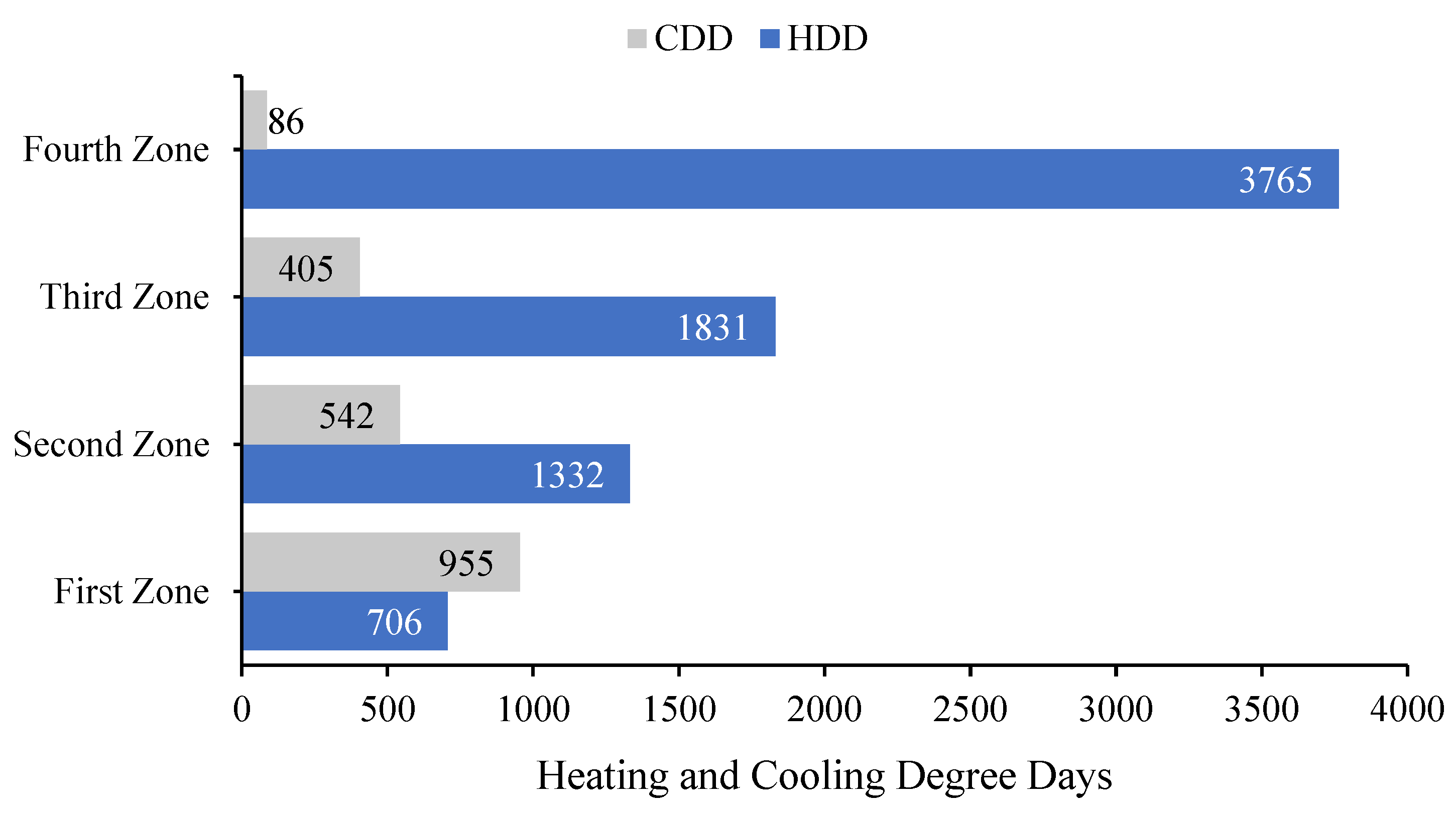
2.1. Degree-Day Method Incorporating Solar Radiation Effect
2.2. Determination of Annual Heat Loss and Gain through Building Walls
2.3. Economic Assessment and CO2 Emission Calculations

| Heating Source | Emission Factor, fh | Lower Heating Value, Hu | Efficiency, η | Price, Cf |
|---|---|---|---|---|
| (kgCO2/kWh) | (%) | |||
| Natural Gas | 0.194 | 34.526 × 10⁶ J/m3 | 93 | 0.327 USD/m3 |
| Electricity | 0.588 | 3.599 × 10⁶ J/kWh | 99 | 0.1059 USD/kWh |
| Fuel Oil | 0.268 | 40.594 × 10⁶ J/kg | 80 | 0.734 USD/kg |
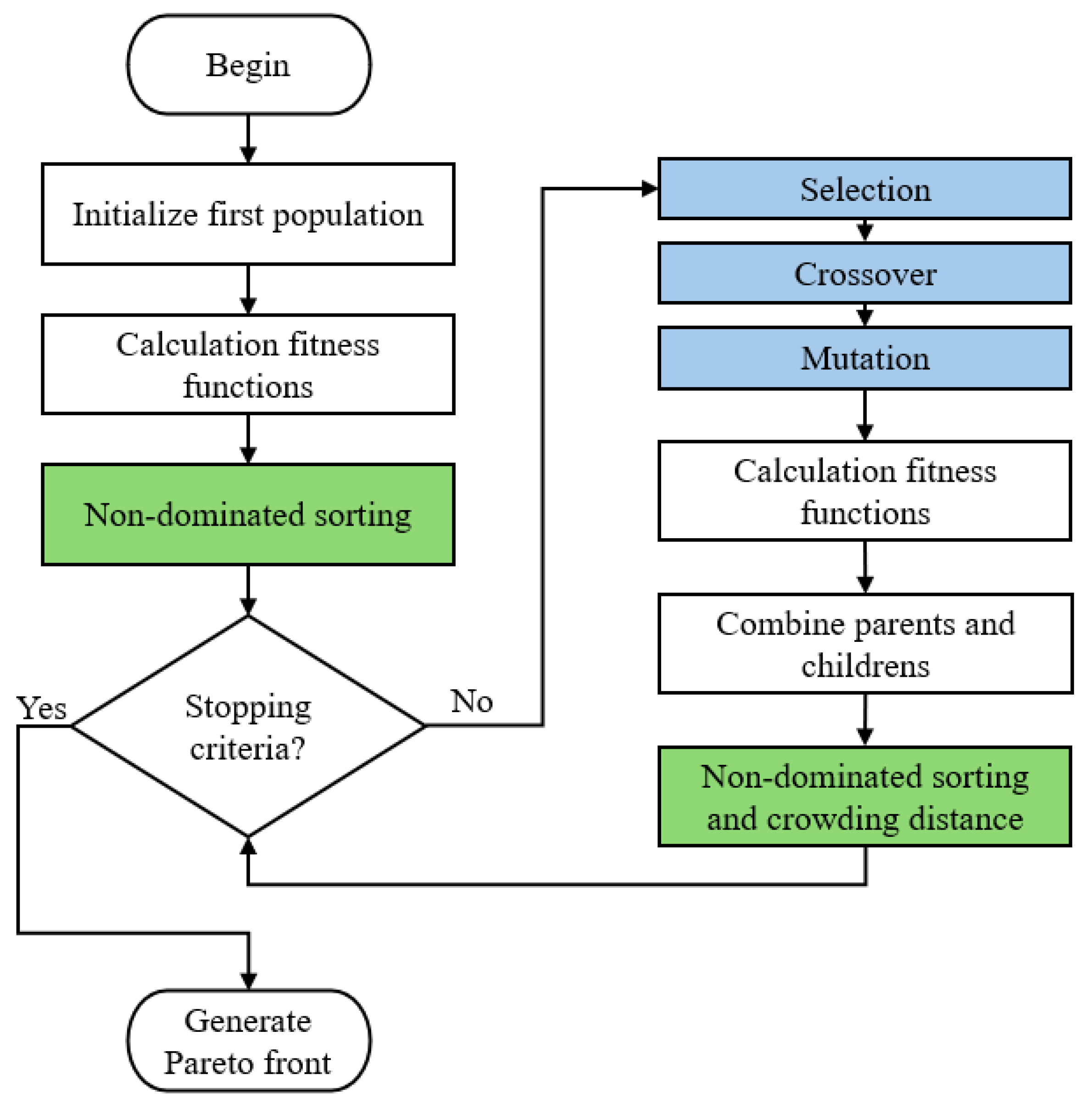
2.4. Multi-Objective Optimization and Knee Point
3. Results and Discussion
4. Conclusions
Author Contributions
Funding
Institutional Review Board Statement
Informed Consent Statement
Data Availability Statement
Conflicts of Interest
References
- Zamorano, M. Recent Advances in Energy Efficiency of Buildings. Appl. Sci. 2022, 12, 6669. [Google Scholar] [CrossRef]
- Mohkam, M.; Mohammadi, S.M.H.; Arababadia, R.; Jahanshahi Javaran, E. Impacts of phase change materials on performance of operational peak load shifting strategies in a sample building in hot-arid climate. Environ. Prog. Sustain. Energy 2023, 42, e13961. [Google Scholar] [CrossRef]
- Asdrubali, F.; D’Alessandro, F.; Schiavoni, S. A review of unconventional sustainable building insulation materials. Sustain. Mater. Technol. 2015, 4, 1–17. [Google Scholar] [CrossRef]
- Braulio-Gonzalo, M.; Bovea, M.D. Environmental and cost performance of building’s envelope insulation materials to reduce energy demand: Thickness optimisation. Energy Build. 2017, 150, 527–545. [Google Scholar] [CrossRef]
- Dylewski, R. Optimal thermal insulation thicknesses of external walls based on economic and ecological heating cost. Energies 2019, 12, 3415. [Google Scholar] [CrossRef]
- Ali, K.A.; Ahmad, M.I.; Yusup, Y. Issues, impacts, and mitigations of carbon dioxide emissions in the building sector. Sustainability 2020, 12, 7427. [Google Scholar] [CrossRef]
- López-Ochoa, L.M.; Las-Heras-Casas, J.; López-González, L.M.; García-Lozano, C. Energy renovation of residential buildings in cold Mediterranean zones using optimized thermal envelope insulation thicknesses: The case of Spain. Sustainability 2020, 12, 2287. [Google Scholar] [CrossRef]
- Zhu, W.; Feng, W.; Li, X.; Zhang, Z. Analysis of the embodied carbon dioxide in the building sector: A case of China. J. Clean. Prod. 2020, 269, 122438. [Google Scholar] [CrossRef]
- Bharadwaj, P.; Jankovic, L. Self-organised approach to designing building thermal insulation. Sustainability 2020, 12, 5764. [Google Scholar] [CrossRef]
- Li, D.; Huang, Y.; Guo, C.; Wang, H.; Jia, J.; Huang, L. Low-Carbon Optimization Design for Low-Temperature Granary Roof Insulation in Different Ecological Grain Storage Zones in China. Sustainability 2023, 15, 13626. [Google Scholar] [CrossRef]
- Min, J.; Yan, G.; Abed, A.M.; Elattar, S.; Amine Khadimallah, M.; Jan, A.; Ali, H.E. The effect of carbon dioxide emissions on the building energy efficiency. Fuel 2022, 326, 124842. [Google Scholar] [CrossRef]
- Er-rradi, H.; Idchabani, R.; Oubrek, M.; Bojji, C.; Boukhattem, L.; Doublali, A.; Jilbab, A. Experimental study of composite materials based on ecological wastes. J. Compos. Mater. 2022, 56, 3295–3306. [Google Scholar] [CrossRef]
- Wang, X.; Lin, Q.; Li, J. Energy Saving Technology of Wall Insulation of Harbor Building Based on Energy Cost Analysis. Therm. Sci. 2021, 26, 4003–4010. [Google Scholar] [CrossRef]
- Stamoulis, M.N.; dos Santos, G.H.; Lenz, W.B.; Tusset, A.M. Genetic algorithm applied to multi-criteria selection of thermal insulation on industrial shed roof. Buildings 2019, 9, 238. [Google Scholar] [CrossRef]
- Bolattürk, A. Optimum insulation thicknesses for building walls with respect to cooling and heating degree-hours in the warmest zone of Turkey. Build. Environ. 2008, 43, 1055–1064. [Google Scholar] [CrossRef]
- Kaynakli, O. A study on residential heating energy requirement and optimum insulation thickness. Renew. Energy 2008, 33, 1164–1172. [Google Scholar] [CrossRef]
- Ozel, M. Thermal performance and optimum insulation thickness of building walls with different structure materials. Appl. Therm. Eng. 2011, 31, 3854–3863. [Google Scholar] [CrossRef]
- Dylewski, R.; Adamczyk, J. Economic and Ecological Optimization of Thermal Insulation Depending on the Pre-Set Temperature in a Dwelling. Energies 2023, 16, 4174. [Google Scholar] [CrossRef]
- Kotb, A.T.M.; Nawar, M.A.A.; Attai, Y.A.; Mohamed, M.H. Performance enhancement of a Wells turbine using CFD-optimization algorithms coupling. Energy 2023, 282, 128962. [Google Scholar] [CrossRef]
- Zheng, Z.; Xiao, J.; Yang, Y.; Xu, F.; Zhou, J.; Liu, H. Optimization of exterior wall insulation in office buildings based on wall orientation: Economic, energy and carbon saving potential in China. Energy 2024, 290, 130300. [Google Scholar] [CrossRef]
- Çallı, M.; Albak, E.İ.; Öztürk, F. Prediction and Optimization of the Design and Process Parameters of a Hybrid DED Product Using Artificial Intelligence. Appl. Sci. 2022, 12, 5027. [Google Scholar] [CrossRef]
- Tunçel, O. Optimization of Charpy Impact Strength of Tough PLA Samples Produced by 3D Printing Using the Taguchi Method. Polymers 2024, 16, 459. [Google Scholar] [CrossRef]
- Canbolat, A.S.; Bademlioglu, A.H.; Kaynakli, O. Thermohydraulic Performance Optimization of Automobile Radiators Using Statistical Approaches. J. Therm. Sci. Eng. Appl. 2022, 14, 051014. [Google Scholar] [CrossRef]
- Albak, E.İ. Optimization for multi-cell thin-walled tubes under quasi-static three-point bending. J. Brazilian Soc. Mech. Sci. Eng. 2022, 44, 207. [Google Scholar] [CrossRef]
- Wu, Y.; Li, Z.; Zhang, B.; Chen, H.; Sun, Y. Multi-objective optimization of key parameters of stirred tank based on ANN-CFD. Powder Technol. 2024, 441, 119832. [Google Scholar] [CrossRef]
- Gao, B.; Zhu, X.; Ren, J.; Ran, J.; Kim, M.K.; Liu, J. Multi-objective optimization of energy-saving measures and operation parameters for a newly retrofitted building in future climate conditions: A case study of an office building in Chengdu. Energy Rep. 2023, 9, 2269–2285. [Google Scholar] [CrossRef]
- Behzadi Hamooleh, M.; Torabi, A.; Baghoolizadeh, M. Multi-objective optimization of energy and thermal comfort using insulation and phase change materials in residential buildings. Build. Environ. 2024, 262, 111774. [Google Scholar] [CrossRef]
- Alimohamadi, R.; Jahangir, M.H. Multi-Objective optimization of energy consumption pattern in order to provide thermal comfort and reduce costs in a residential building. Energy Convers. Manag. 2024, 305, 118214. [Google Scholar] [CrossRef]
- Bi, H.; Lu, F.; Duan, S.; Huang, M.; Zhu, J.; Liu, M. Two-level principal–agent model for schedule risk control of IT outsourcing project based on genetic algorithm. Eng. Appl. Artif. Intell. 2020, 91, 103584. [Google Scholar] [CrossRef]
- Antonio, L.M.; Coello, C.A.C. Use of cooperative coevolution for solving large scale multiobjective optimization problems. In Proceedings of the 2013 IEEE Congress on Evolutionary Computation, Cancun, Mexico, 20–23 June 2013; pp. 2758–2765. [Google Scholar] [CrossRef]
- de Farias, L.R.C.; Araújo, A.F.R. A decomposition-based many-objective evolutionary algorithm updating weights when required. Swarm Evol. Comput. 2022, 68, 100980. [Google Scholar] [CrossRef]
- Liu, Y.; Ishibuchi, H.; Masuyama, N.; Nojima, Y. Adapting Reference Vectors and Scalarizing Functions by Growing Neural Gas to Handle Irregular Pareto Fronts. IEEE Trans. Evol. Comput. 2020, 24, 439–453. [Google Scholar] [CrossRef]
- Canbolat, A.S. An integrated assessment of the financial and environmental impacts of exterior building insulation application. J. Clean. Prod. 2023, 435, 140376. [Google Scholar] [CrossRef]
- Kurekci, N.A. Determination of optimum insulation thickness for building walls by using heating and cooling degree-day values of all Turkey’s provincial centers. Energy Build. 2016, 118, 197–213. [Google Scholar] [CrossRef]
- Canbolat, A.; Bademlioglu, A.; Saka, K.; Kaynakli, O. Investigation of parameters affecting the optimum thermal insulation thickness for buildings in hot and cold climates. Therm. Sci. 2020, 24, 2891–2903. [Google Scholar] [CrossRef]
- Bektas Ekici, B.; Aytac Gulten, A.; Aksoy, U.T. A study on the optimum insulation thicknesses of various types of external walls with respect to different materials, fuels and climate zones in Turkey. Appl. Energy 2012, 92, 211–217. [Google Scholar] [CrossRef]
- Corrales-Suastegui, A.; Ruiz-Alvarez, O.; Torres-Alavez, J.A.; Pavia, E.G. Analysis of cooling and heating degree days over mexico in present and future climate. Atmosphere 2021, 12, 1131. [Google Scholar] [CrossRef]
- Cengel, Y. Heat Transfer: A Practical Approach, 2nd ed.; McGraw-Hill: New York, NY, USA, 2002. [Google Scholar]
- Tiris, M.; Tiris, Ç.; Türe, I.E. Diffuse solar radiation correlations: Applications to Turkey and Australia. Energy 1995, 20, 745–749. [Google Scholar] [CrossRef]
- Yiğit, A.; Atmaca, İ. Solar Energy; Alfa Aktüel: Bursa, Turkey, 2010. (In Turkish) [Google Scholar]
- Kaynakli, Ö.; Kaynakli, F. Determination of Optimum Thermal Insulation Thicknesses for External Walls Considering The Heating, Cooling and Annual Energy Requirements. Uludağ Univ. J. Fac. Eng. 2016, 21, 229. [Google Scholar] [CrossRef]
- Central Bank of Türkiye. Available online: https://www.tcmb.gov.tr (accessed on 5 April 2024).
- Turkish Statistical Institute. Available online: www.tuik.gov.tr (accessed on 12 November 2023).
- Ucar, A.; Balo, F. Determination of the energy savings and the optimum insulation thickness in the four different insulated exterior walls. Renew. Energy 2010, 35, 88–94. [Google Scholar] [CrossRef]
- Anastaselos, D.; Giama, E.; Papadopoulos, A.M. An assessment tool for the energy, economic and environmental evaluation of thermal insulation solutions. Energy Build. 2009, 41, 1165–1171. [Google Scholar] [CrossRef]
- Saafi, K.; Daouas, N. A life-cycle cost analysis for an optimum combination of cool coating and thermal insulation of residential building roofs in Tunisia. Energy 2018, 152, 925–938. [Google Scholar] [CrossRef]
- Zroichikov, N.A.; Gribkov, A.M.; Saparov, M.I.; Mirsalikhov, K.M. A General-Purpose Procedure for the Calculation of the Optimum Gas Velocity in Gas Exhaust Ducts of Stacks at Thermal Power Stations. Therm. Eng. 2020, 67, 157–164. [Google Scholar] [CrossRef]
- Asadi, I.; Shafigh, P.; Abu Hassan, Z.F.B.; Mahyuddin, N.B. Thermal conductivity of concrete—A review. J. Build. Eng. 2018, 20, 81–93. [Google Scholar] [CrossRef]
- Liu, H.; Li, Q.; Quan, H.; Xu, X.; Wang, Q.; Ni, S. Assessment on the Properties of Biomass-Aggregate Geopolymer Concrete. Appl. Sci. 2022, 12, 3561. [Google Scholar] [CrossRef]
- Axaopoulos, I.; Axaopoulos, P.; Gelegenis, J.; Fylladitakis, E.D. Optimum external wall insulation thickness considering the annual CO2 emissions. J. Build. Phys. 2019, 42, 527–544. [Google Scholar] [CrossRef]
- Tian, Y.; Cheng, R.; Zhang, X.; Jin, Y. PlatEMO: A MATLAB Platform for Evolutionary Multi-Objective Optimization [Educational Forum]. IEEE Comput. Intell. Mag. 2017, 12, 73–87. [Google Scholar] [CrossRef]
- Deb, K.; Pratap, A.; Agarwal, S.; Meyarivan, T. A fast and elitist multiobjective genetic algorithm: NSGA-II. IEEE Trans. Evol. Comput. 2002, 6, 182–197. [Google Scholar] [CrossRef]
- Peng, Y.; Wang, S.; Yao, S.; Xu, P. Crashworthiness analysis and optimization of a cutting-style energy absorbing structure for subway vehicles. Thin-Walled Struct. 2017, 120, 225–235. [Google Scholar] [CrossRef]
- Duan, S.; Tao, Y.; Han, X.; Yang, X.; Hou, S.; Hu, Z. Investigation on structure optimization of crashworthiness of fiber reinforced polymers materials. Compos. Part. B Eng. 2014, 60, 471–478. [Google Scholar] [CrossRef]
- TS 825; Thermal Insulation Requirements for Buildings. Turkish Standards Institution: Ankara, Turkey, 2013.
- Sisman, N.; Kahya, E.; Aras, N.; Aras, H. Determination of optimum insulation thicknesses of the external walls and roof (ceiling) for Turkey’s different degree-day regions. Energy Policy 2007, 35, 5151–5155. [Google Scholar] [CrossRef]
- Ucar, A. Thermoeconomic analysis method for optimization of insulation thickness for the four different climatic regions of Turkey. Energy 2010, 35, 1854–1864. [Google Scholar] [CrossRef]
- Ozbek, K.; Gelis, K.; Ozyurt, O. Optimization of external wall insulation thickness in buildings using response surface methodology. Int. J. Energy Environ. Eng. 2022, 13, 1367–1381. [Google Scholar] [CrossRef]


| Wall Components | Emission Factor, f | Density, ρ | Conductivity, k | Price, C |
|---|---|---|---|---|
| (kgCO2/kg) | (kg/m3) | (W/mK) | (USD/m3) | |
| Expanded Polystyrene (EPS) | 3.51 | 20 | 0.036 | 100 |
| Extruded Polystyrene (XPS) | 3.83 | 30 | 0.037 | 150 |
| Mineral Wool (MW) | 1.16 | 55 | 0.04 | 130 |
| Polyurethane Foam (PUR) | 4.47 | 40 | 0.036 | 200 |
| Plaster | 0.36 | 1800 | 0.87 | 90 |
| Light Concrete | 0.09 | 1700 | 0.71 | 85 |
| Reinforced Concrete | 0.12 | 2400 | 2.5 | 120 |
| Brick | 0.31 | 1200 | 0.45 | 45 |
| Insulation Thickness (m) | Insulation Material | Wall Material | Heating Source | |
|---|---|---|---|---|
| Base Case Scenario | 0.02 | XPS | Brick | Fuel Oil |
| Optimum Cost | 0.0470 | EPS | Brick | Natural Gas |
| Optimum CO2 | 0.1961 | EPS | Light concrete | Natural Gas |
| Cost-Oriented Knee Point | 0.1312 | EPS | Brick | Natural Gas |
| CO2-Oriented Knee Point | 0.0790 | EPS | Light concrete | Natural Gas |
| Method | Scenario | CT (USD/m2) | MCO2 (kg/m2) | % CT | % MCO2 |
|---|---|---|---|---|---|
| Base Case Scenario | 42.60 | 20.14 | - | - | |
| CCGDE3 | Optimum Cost | 34.27 | 15.56 | 20% | 23% |
| Optimum CO2 | 52.44 | 9.18 | −23% | 54% | |
| MOEA/D-UR | Optimum Cost | 34.27 | 15.55 | 20% | 23% |
| Optimum CO2 | 52.41 | 9.18 | −23% | 54% | |
| DEA-GNG | Optimum Cost | 34.27 | 15.55 | 20% | 23% |
| Optimum CO2 | 52.45 | 9.18 | −23% | 54% | |
| NSGA-II | Optimum Cost | 34.27 | 15.50 | 20% | 23% |
| Optimum CO2 | 52.45 | 9.18 | −23% | 54% | |
| Cost-Oriented Knee Point | 38.84 | 13.68 | 9% | 32% | |
| CO2-Oriented Knee Point | 43.56 | 10.17 | −2% | 50% |
| Insulation Thickness (m) | Insulation Material | Wall Material | Heating Source | |
|---|---|---|---|---|
| Base Case Scenario | 0.02 | XPS | Brick | Fuel Oil |
| Optimum Cost | 0.0499 | EPS | Brick | Natural Gas |
| Optimum CO2 | 0.2055 | EPS | Light concrete | Natural Gas |
| Cost-Oriented Knee Point | 0.1368 | EPS | Brick | Natural Gas |
| CO2-Oriented Knee Point | 0.0829 | EPS | Light concrete | Natural Gas |
| Method | Scenario | CT (USD/m2) | MCO2 (kg/m2) | % CT | % MCO2 |
|---|---|---|---|---|---|
| Base Case Scenario | 48.45 | 22.40 | - | - | |
| CCGDE3 | Optimum Cost | 34.84 | 15.79 | 28% | 30% |
| Optimum CO2 | 53.44 | 9.31 | 28% | 30% | |
| MOEA/D-UR | Optimum Cost | 34.84 | 15.79 | 28% | 30% |
| Optimum CO2 | 53.44 | 9.31 | 28% | 30% | |
| DEA-GNG | Optimum Cost | 34.84 | 15.80 | 28% | 30% |
| Optimum CO2 | 53.47 | 9.31 | 28% | 30% | |
| NSGA-II | Optimum Cost | 34.84 | 15.79 | 28% | 30% |
| Optimum CO2 | 53.47 | 9.31 | −10% | 58% | |
| Cost-Oriented Knee Point | 39.51 | 13.83 | 18% | 38% | |
| CO2-Oriented Knee Point | 44.16 | 10.36 | 9% | 54% |
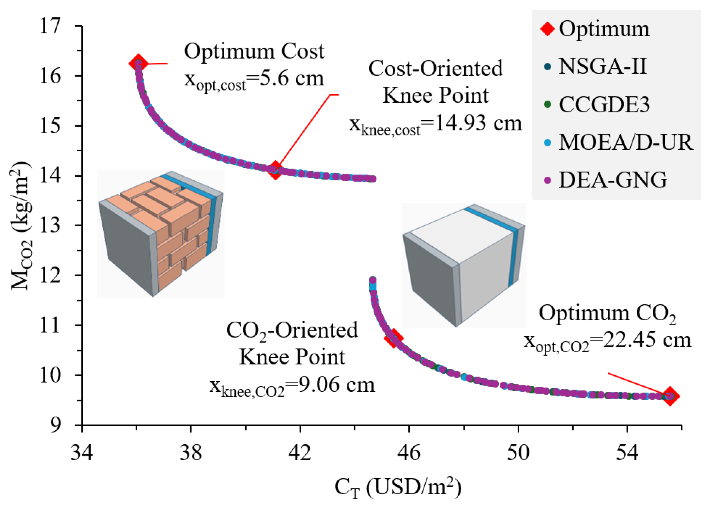
| Insulation Thickness (m) | Insulation Material | Wall Material | Heating Source | |
|---|---|---|---|---|
| Base Case Scenario | 0.02 | XPS | Brick | Fuel Oil |
| Optimum Cost | 0.056 | EPS | Brick | Natural Gas |
| Optimum CO2 | 0.2245 | EPS | Light concrete | Natural Gas |
| Cost-Oriented Knee Point | 0.1493 | EPS | Brick | Natural Gas |
| CO2-Oriented Knee Point | 0.0906 | EPS | Light concrete | Natural Gas |
| Method | Scenario | CT (USD/m2) | MCO2 (kg/m2) | % CT | % MCO2 |
|---|---|---|---|---|---|
| Base Case Scenario | 54.52 | 25.10 | - | - | |
| CCGDE3 | Optimum Cost | 36.07 | 16.26 | 34% | 35% |
| Optimum CO2 | 55.62 | 9.58 | −2% | 62% | |
| MOEA/D-UR | Optimum Cost | 36.07 | 16.24 | 34% | 35% |
| Optimum CO2 | 55.50 | 9.58 | −2% | 62% | |
| DEA-GNG | Optimum Cost | 36.07 | 16.24 | 34% | 35% |
| Optimum CO2 | 55.57 | 9.58 | −2% | 62% | |
| NSGA-II | Optimum Cost | 36.07 | 16.25 | 34% | 35% |
| Optimum CO2 | 55.57 | 9.58 | −2% | 62% | |
| Cost-Oriented Knee Point | 41.10 | 14.11 | 25% | 44% | |
| CO2-Oriented Knee Point | 45.42 | 10.74 | 17% | 57% |
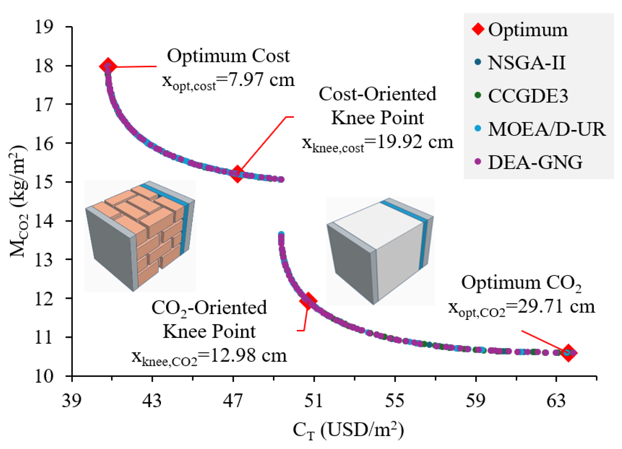
| Insulation Thickness (m) | Insulation Material | Wall Material | Heating Source | |
|---|---|---|---|---|
| Base Case Scenario | 0.02 | XPS | Brick | Fuel Oil |
| Optimum Cost | 0.0797 | EPS | Brick | Natural Gas |
| Optimum CO2 | 0.2971 | EPS | Light concrete | Natural Gas |
| Cost-Oriented Knee Point | 0.1992 | EPS | Brick | Natural Gas |
| CO2-Oriented Knee Point | 0.1298 | EPS | Light concrete | Natural Gas |
| Method | Scenario | CT (USD/m2) | MCO2 (kg/m2) | % CT | % MCO2 |
|---|---|---|---|---|---|
| Base Case Scenario | 79.66 | 36.58 | - | - | |
| CCGDE3 | Optimum Cost | 40.80 | 17.97 | 49% | 51% |
| Optimum CO2 | 63.64 | 10.60 | 20% | 71% | |
| MOEA/D-UR | Optimum Cost | 40.80 | 17.97 | 49% | 51% |
| Optimum CO2 | 63.52 | 10.60 | 20% | 71% | |
| DEA-GNG | Optimum Cost | 40.80 | 17.97 | 49% | 51% |
| Optimum CO2 | 63.84 | 10.60 | 20% | 71% | |
| NSGA-II | Optimum Cost | 40.80 | 17.97 | 49% | 51% |
| Optimum CO2 | 63.60 | 10.60 | 20% | 71% | |
| Cost-Oriented Knee Point | 47.21 | 15.20 | 41% | 58% | |
| CO2-Oriented Knee Point | 50.71 | 11.93 | 36% | 67% |
Disclaimer/Publisher’s Note: The statements, opinions and data contained in all publications are solely those of the individual author(s) and contributor(s) and not of MDPI and/or the editor(s). MDPI and/or the editor(s) disclaim responsibility for any injury to people or property resulting from any ideas, methods, instructions or products referred to in the content. |
© 2024 by the authors. Licensee MDPI, Basel, Switzerland. This article is an open access article distributed under the terms and conditions of the Creative Commons Attribution (CC BY) license (https://creativecommons.org/licenses/by/4.0/).
Share and Cite
Canbolat, A.S.; Albak, E.İ. Multi-Objective Optimization of Building Design Parameters for Cost Reduction and CO2 Emission Control Using Four Different Algorithms. Appl. Sci. 2024, 14, 7668. https://doi.org/10.3390/app14177668
Canbolat AS, Albak Eİ. Multi-Objective Optimization of Building Design Parameters for Cost Reduction and CO2 Emission Control Using Four Different Algorithms. Applied Sciences. 2024; 14(17):7668. https://doi.org/10.3390/app14177668
Chicago/Turabian StyleCanbolat, Ahmet Serhan, and Emre İsa Albak. 2024. "Multi-Objective Optimization of Building Design Parameters for Cost Reduction and CO2 Emission Control Using Four Different Algorithms" Applied Sciences 14, no. 17: 7668. https://doi.org/10.3390/app14177668