Abstract
Accurate evapotranspiration (ET) estimation is crucial for sustainable water management in the diverse and water-scarce Mediterranean region. This study compares three prominent models (Simulator of Terrestrial Ecohydrological Processes and Systems (STEPS), Soil-Canopy-Observation of Photosynthesis and Energy fluxes (SCOPE), and Two-Source Energy Balance (TSEB)) with established global datasets (Moderate Resolution Imaging Spectroradiometer 8-day global terrestrial product (MOD16A2), Global Land Evaporation Amsterdam Model (GLEAM), and TerraClimate) at multiple spatial and temporal scales and validates model outcomes with eddy covariance based ground measurements. Insufficient ground-based observations limit comprehensive model validation in the eastern Mediterranean part (Turkey and Balkans). The results reveal significant discrepancies among models and datasets, highlighting the challenges of capturing ET variability in this complex region. Differences are attributed to variations in ecosystem type, energy balance calculations, and water availability constraints. Ground validation shows that STEPS performs well in some French and Italian forests and crops sites but struggles with seasonal ET patterns in some locations. SCOPE mostly overestimates ET due to detailed radiation flux calculations and lacks accurate water limitation representation. TSEB faces challenges in capturing ET variations across different ecosystems at a coarser 10 km resolution. No single model and global dataset accurately represent ET across the entire region. Model performance varies by region and ecosystem. As GLEAM and TSEB excel in semi-arid Savannahs, STEPS and SCOPE are better in grasslands, croplands, and forests in few locations (5 out of 18 sites) which indicates these models need calibration for other locations and ecosystem types. Thus, a region-specific model calibration and validation, sensitive to extremely humid and arid conditions can improve ET estimation across the diverse Mediterranean region.
1. Introduction
Evapotranspiration (ET) is a critical component of the hydrological cycle, deeply influencing water availability in ecosystems and agricultural landscapes []. Yet, predicting ET on a large scale is quite challenging, given the myriad of physical drivers at play. Factors such as wind patterns, cloud cover, soil moisture, surface albedo, precipitation, radiation scattering, and surface heterogeneity introduce considerable variability. Moreover, the intricate interplay of crop biophysical characteristics, including canopy structure, vegetation abundance, phenology, and energy partitioning, further compounds this variability. This complexity is especially pronounced in data-sparse regions and heterogeneous land use systems, such as the Mediterranean region []. This region experiences a complex interplay of factors, including diverse land cover, heterogeneous topography, and variable climatic conditions, making ET estimation particularly challenging []. Moreover, ET and precipitation are the principal mechanisms of the water balance in the Mediterranean Basin. Due to precipitation decline, Mediterranean ecosystems in specific arid and semi-arid production systems are more vulnerable to water stress leading to growing hydrological imbalances in the basin []. The accelerating near-surface temperatures and declining near-surface soil moisture exacerbate the need for precise ET assessments []. Our understanding of Mediterranean ecosystems’ reactions to stressed hydro-climatological conditions is still limited. This information gap demands strong monitoring and modeling capabilities in terrestrial water flux quantification (evapotranspiration, runoff, and groundwater storage), especially ET, which is a principal water-extracting component in arid regions. ET’s accurate quantification with precipitation is becoming critical in the basin with the growing water and food scarcity [,]. Since many ET modeling schemes exist, it is meaningful to find the best approach for the Mediterranean region through which we can manage and control water stress, seasonal water shortages, and the expansion of irrigated agriculture.
While various remote sensing and modeling approaches have been developed to estimate ET, their effectiveness in capturing the complexities of the Mediterranean region is still negotiable. Remote sensing-based models often rely on empirical relationships and simplifications, neglecting the influence of sub-surface hydrology and complex land use patterns. ET by these models is derived from the integration of radiometric land surface temperature (LST), and biophysical variables, i.e., leaf area index (LAI), photosynthetically active radiation (PAR), fractional vegetation cover (FVC), clumping index, leaf angles, canopy height, leaf abundance, ecosystem hierarchy, etc. [,]. Some other techniques are based on net radiation and temperature differentials [,], or an inferential approach constrained by crop coefficients [,,]. These simple generic models do not account for the horizontal movement of soil energy fluxes and water and heat storage [,,,]. Some examples are the Mapping ET at high Resolution with Internalized Calibration-Earth Engine Evapotranspiration Flux (METRIC-EEFlux), surface energy balance index (SEBI), Operational Simplified Surface Energy Balance (SSEBop), Atmosphere-Land Exchange Inverse algorithm (ALEXI), and Atmosphere Land Exchange Inverse Disaggregation algorithm (DisALEXI). In these models, LST is used as a proxy for soil moisture conditions of the upper soil layer. Surface resistances are modeled as a function of abstracted hydrology following the aerodynamic theory. The accurate estimation of aerodynamic resistance is crucial, due to complexities in atmospheric conditions and surface characteristics. Temperature gradients in the planetary boundary layer influence the rate of evaporation, and changes in surface roughness occur as soil moisture decreases and vegetation wilt, further affecting the exchange of moisture between the surface and the atmosphere. Though these models have made ET determination easier are more flexible in time and scale. With their generic settings, they have been applied over large continents in recent years such as Water Productivity Open-access portal version 2 (WaPORII) for Africa, the Global Daily Evapotranspiration Portal-Atmosphere-Land Exchange Inverse algorithm (GLODET-ALEXI) for the Mediterranean region, and OpenET-Ensemble for the United States Continent [,]. The lack of uniformity in the current model schemes made ET estimates more uncertain. LST-driven models do not have soil–water balancing and are preferred to use in crop ET monitoring due to their short temporal frequency and compatibility with crop phenology. Where ET in the semi-arid Mediterranean environment is very sensitive to soil moisture conditions, sub-surface hydrology in the soil plays a significant role in ET regulation [,,,,]. ET methods need to increase their modeling precision in stress parameters and better space/time resolutions with good-quality data to improve the quality of predictions in water-stressed environments.
Physically based soil–vegetation–atmosphere transfer (SVAT) models offer a more mechanistic representation of hydrological processes, coupling soil moisture dynamics, root zone interactions, and energy balance components. However, their application to diverse land use systems, such as rotational cropping, demands extensive parameterization and a large variable space []. Large-scale applications require multi-calibration techniques to enhance ET accuracy within a hydrological model because SVAT models often struggle to accurately capture ET in complex and heterogeneous landscapes []. The weak correlation between root zone soil moisture and canopy temperature under water-stressed conditions further emphasizes the challenges associated with these models []. Some SVAT modeling schemes use coupled Penman-Monteith and water balance approaches in a spatially explicit manner and simulate the coupled interactions between water and energy regimes. Such schemes connect deep soil hydrology with atmospheric fluxes realistically, they often require trial and error-based intensive parameterization with a comparatively large number of datasets [,]. This study intends to explore which ET estimation approach is most suitable for the Mediterranean region in capturing spatial variability of ET across different ecosystems. With that aim, models based on energy balance, water balance, and coupled approaches are tested in which the first large-scale application of the SVAT model, STEPS, to the Mediterranean region is introduced with its comparison with other established models, i.e., SCOPE and TSEB.
STEPS is a process-based model that dynamically calculates lateral water movement, runoff, soil moisture content, water table depth, and snowmelt, and integrates it all together and estimates ET on a daily scale. It adopts a “four-leaf” approach to stratify leaves based on moisture and sunlit conditions and solves water balance equations for each depth of the soil layer to represent diverse ecological and hydrological constraints in a spatially explicit manner []. Simulating the coupled behavior of water and energy cycle and accounting for subsurface lateral flux movement differentiates it from SCOPE and TSEB. In contrast, the SCOPE, being a radiative transfer model with energy balance calculations, first simulates spectral reflectance and transmittance of vegetation canopy and soil to derive fluxes of radiation, heat, water vapor, and carbon dioxide in the soil–atmosphere–vegetation continuum. It uses empirical and semi-empirical relationships and parameterizes the effects of soil moisture and LAI on canopy conductance and photosynthesis. However, it does not address the topography or canopy-clumping effects that STEPS do []. TSEB, in comparison, is a simple dual-source energy balance model that estimates two-layer evaporation separately for soil and canopy from the satellite-based LST in which wind speed and canopy height are used to compute aerodynamic and surface resistances. It simulates turbulent fluxes in the loop of given boundary layer conditions and uses empirical and semi-empirical relationships to parameterize the effects of surface temperature, vegetation cover, and aerodynamic resistance on the energy fluxes. In TSEB, the choice of soil resistance formulation can affect the accuracy of ET estimation. Different studies proposed and evaluated different soil resistance formulations []. Apart from others, it has the flexibility of choosing different ET methods, i.e., the Priestley–Taylor equation, dual-time difference approach, or component soil and canopy temperatures approach; all these methods require different climatic inputs, such as the maximum and the minimum air temperature, solar radiation, relative humidity, wind speed, etc. All these models are unique in their ET determination methods, input data, output frequency, assumptions, and sources of uncertainty.
This study evaluates the performances of these ET models (STEPS, SCOPE, and TSEB) across the Mediterranean region and compares them with those of existing global ET products (MOD16A2, GLEAM, and TerraClimate) and ground-based measurements, to identify their strengths, weaknesses, and potential for ET estimation in this complex environment. In the literature, mostly a comparison of annual and monthly estimates has been provided. This study provides a deeper insight into the modeled ET at a sub-regional scale to see if the modeled ET is reliable for all regions. This is a concern because low accuracy can change the water budget estimate if ET is not modeled accurately, and if some environmental constraints are ignored especially in arid and humid climates. Thus, our research contributes to a better understanding of ET dynamics in the Mediterranean region to support informed water resource management.
2. Materials and Methods
2.1. Common Inputs for STEPS, SCOPE, and TSEB
In the first step, daily meteorological data are prepared by aggregating the hourly 5th generation ECMWF Reanalysis for the Global Climate and Weather data (ERA5), United Kingdom [] in the Google Earth Engine (GEE) platform. These data are used as a common meteorological input for all models. ERA5 is chosen due to its global coverage and efficacy for data-sparse areas. Some discrepancies observed in the ERA5 repository in GEE led us to cross-check a portion of ERA5-Land data “ECMWF/ERA5_LAND/HOURLY” against the official Copernicus Climate Data Store for consistency. The pre-processing of ERA5 was carried out following the method in [].
For TSEB, hourly ERA5 weather data [air temperature, wind speed, and vapor pressure forcing] and LST from the Spinning Enhanced Visible and InfraRed Imager (SEVIRI), France on board the Meteosat Second Generation MSG were used to calculate instantaneous ET at 12:00 UTC, using Sentinels for the ET method (Sen-ET). These hourly variables are processed at the 100 m atmospheric blending height above the surface. TSEB also uses a different source of radiation data. Both instantaneous and daily average downward shortwave radiation input of TSEB are from MSG, i.e., the Total and Diffuse Downward Surface Shortwave Flux product (https://landsaf.ipma.pt/en/products/longwave-shortwave-radiation/mdssftd/) accessed on 1 November 2022. Their daily average is used to upscale the TSEB’s instantaneous ET to a daily ET following the method in [].
For STEPS, we used daily maximum, minimum, and average temperature (°C), median dew point (°C), total precipitation (mm), wind speed (ms−1), and total short-wave radiation (Wm2). A list of these datasets is in Table 1 showing input variables for each model.

Table 1.
ERA5: hourly climate datasets and other surface parameters used in three models input listed with their names and units.
Other ready-to-use datasets like Precipitation from Soil Moisture to Rain (SM2Rain) [] and Hourly Potential Evapotranspiration at 0.1-degree resolution [] were obtained from (https://doi.org/10.5281/zenodo.846259 accessed on 5 November 2022; https://data.bris.ac.uk/data/dataset/qb8ujazzda0s2aykkv0oq0ctp) accessed on 1 November 2022to use in water stress assessments.
2.2. Model Input Specifications and Parameterization for STEPS, SCOPE, and TSEB
Particular attention is given to the specific inputs of STEPS, SCOPE, and TSEB and their requirements to ensure transparency over the Mediterranean region. For STEPS, incoming solar radiation is first partitioned into direct and diffuse components using latitude, slope, aspect, and elevation data from the HydroSHEDS Digital Elevation Model (DEM). This partitioning is necessary for canopy radiative transfer calculations, which STEPS employs in its empirical scheme to simulate eco-hydrological processes []. For the parameterization of soil and surface variables, literature-based ranges are selected to determine soil texture–specific hydraulic properties (wilting point, field capacity, porosity, etc.). The same approach is followed for biological parameters, i.e., the maximum carboxylation capacity (Vcmax), canopy clumping index, precipitation interception, and stomatal conductance for each land cover class (forests, croplands, grasslands, and shrublands).
The STEPS model simulates daily LAI values (LAIdaily) using its phenology module. It considers daily air temperature and the maximum LAI (LAImax) of the growing season for each vegetation type and applies the classical growing degree days (GDD) concept, where LAImax is a crucial variable for simulating biophysical processes, i.e., photosynthesis, respiration, etc. []. STEPS and SCOPE both acquired the high-quality maximum LAI product, MOD15A2H V6. While TSEB acquired the daily LAI product from SEVIRI-MSG (https://landsaf.ipma.pt/en/products/vegetation/lai/) accessed on 5 November 2022. Table 2 summarizes the model-specific inputs and model specifications for STEPS, SCOPE, and TSEB.
Table 2.
Modeled ET inputs, frequency, resolution sources, and estimation approach.
To ensure consistency across models, all surface and subsurface parameters were resampled to a fixed 10 km resolution (Table 2). These parameters include the following:
- LAI;
- Volumetric Soil Moisture Content (VSMC) for SCOPE and STEPS;
- International Soil Reference and Information Centre (ISRIC) SoilGrids containing soil texture and soil depth information for STEPS;
- European Space Agency (ESA) Worldcover 100 m land use/cover for STEPS and SCOPE and GLCNMO-LULC for TSEB.
To enhance the accuracy of ET estimations, adjustments were made to the SCOPE and TSEB model outputs. Initial simulations with SCOPE indicated overestimated ET values in dry, arid regions. To address this, additional soil moisture constraints were added from ERA5 data (volumetric soil water content at 0–7 cm depth) to balance the energy budget []. For TSEB, gap-filling was carried out for LST, and cloud-contaminated pixels using a ratio of actual ET to ASCE-based reference ET, assuming this ratio remained constant over ten days; its rational method is explained in [].
2.3. Model-Specific Parameters
The parameterization schemes of STEPS, SCOPE, and TSEB significantly differ, reflecting their unique approaches to ET estimation. STEPS focuses on soil properties and land cover characteristics, utilizing soil hydraulic parameters and land cover-specific canopy physiological attributes. SCOPE adopts a more complex structure with sub-modules for radiative transfer, energy balance, aerodynamics, and leaf biochemistry. TSEB, relatively simpler, relies on energy balance principles, with key parameters including the Priestley–Taylor coefficient (αPT) and soil resistance constants. Despite these differences, generic parameter settings are applied across the Mediterranean region for this study as follows.
Parameters in STEPS cover soil hydraulics for water movement in Table 3. Land cover-specific canopy characteristics (Table 4) like canopy structure by leaf area index, canopy water content, light conditions conducive to optimal photosynthesis, photosynthetically active photon flux density (PPFD), and stomatal conductance coefficients are given in Table 4 for computing photosynthetic and transpiration rates throughout leaf and canopy.
Table 3.
Hydraulic properties of four soil texture classes used in STEPS model.
Table 4.
Biophysical parameterization of the STEPS model specific to major land cover classes.
SCOPE is rather more complex in its parameterization and structure. It has sub-modules for simulating radiative transfer at both leaf and canopy scales, energy balance modeling for leaf and soil temperature simulations, aerodynamics fitting for resistances, and calculations related to leaf biochemistry.
Table 5 provides a detailed reference for key parameters within the SCOPE, in which the canopy roughness length, leaf drag coefficient, maximum carboxylation rate, and parameters related to the Ball–Berry stomatal conductance model are included, their theoretical details are in [,].
Table 5.
List of relevant parameters used for SCOPE simulations.
TSEB requires rather fewer parameters to calculate the latent heat fluxes of soil and canopy (Table 6). One key parameter is the Priestley–Taylor coefficient (αPT) that governs the potential transpiration rate of the canopy based on available energy and vapor pressure deficit (VPD). For this experiment, a uniform value of αPT equal to 1.26 is applied across all vegetation types, except for forest ecosystems, where it is adjusted based on the canopy height [,]. Soil resistance constants (Rs), represented by parameters (b, c), are set at (0.012, 0.0025), which specifies the resistance to water vapor diffusion from the soil surface to the atmosphere. Other parameters such as green vegetation fraction, fractional cover, and effective leaf width are simply derived from satellite-based NDVI and land cover maps where vegetation parameters are assigned based on the look-up table (Table 2) in Guzinski et al. (2020) [].
Table 6.
Parameterization used for TSEB application in Mediterranean region.
2.4. Global Datasets, Their Inputs, and Underlying Approach
Simulated ET from our models was compared with three established global ET datasets: MOD16A2-ET, GLEAM, and TerraClimate. Table 7 summarizes their resolution, temporal frequency, input data, and primary algorithms used for ET estimation. MOD16A2-ET employs the Penman–Monteith approach to derive canopy conductance and ET. It utilizes MODIS land and vegetation products alongside gridded weather data from The Modern-Era Retrospective analysis for Research and Applications, version 2 (MERRA-2) [].
Table 7.
Characteristics of Global ET products used as reference datasets in this study.
The GLEAM product is derived from microwave satellite observations. Vegetation optical depth (VOD) and soil moisture data are sourced from passive and active C- and L-band microwave sensors. GLEAM first calculates cover-dependent potential evaporation rates (Ep) using the Priestley–Taylor (1972) equation based on air temperature and net radiation. This captures sub-grid land cover heterogeneity. Subsequently, Ep is transformed to actual transpiration or bare soil evaporation at each grid cell using a cover-dependent multiplicative stress factor (S) determined by vegetation optical depth (VOD) and root-zone soil moisture [].
TerraClimate is built upon the Thornthwaite water balance model. It integrates soil and land properties with daily climatological data from the GRIDMET-A Dataset of Daily High-Spatial Resolution Surface Meteorological data to provide water budget and recharge estimates for each grid within the surface water flow direction. ET is then derived by solving the water balance equation for each grid, with available soil water capacity acting as a major constraint [].
2.5. Validation of STEPS, SCOPE, and TSEB
For validation, fine-quality level 2 data from 18 Integrated Carbon Observation System (ICOS) sites were downloaded from the DIBAF-ICOS portal for the year 2019. Although eddy covariance observations are available for the Mediterranean region from 1999 to 2021 across 144 sites, much of these data are not publicly accessible or are only available up to 2015 (the eddy flux sites distribution is shown in Figure 1).
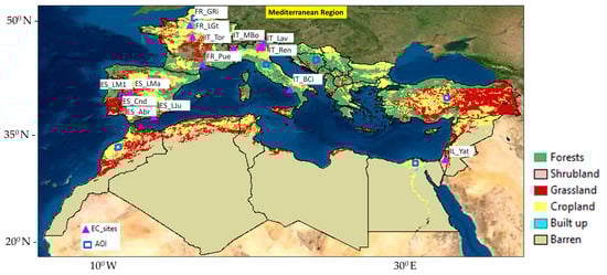
Figure 1.
The figure shows the study area, locations of seven AOIs colored in blue capturing major land use types of Mediterranean countries, and locations of eddy covariance sites in purple from where ground ET is retrieved for validating the results.
In sites where eddy covariance-based ground (G) flux data were available, energy balance closure correction was applied to validate energy balance. These validation datasets were screened for missing values, and the screened LE flux was multiplied with a conversion factor (the latent heat of vaporization) to obtain ET values in millimeters per day.
The daily ET pixels of models were validated against ground-based ET flux measurements to assess model performance in specific ecosystems and compare their differences at sites and regional scales. For this statistical comparison, the determination of coefficients (r2), root mean square error (RMSE), and mean bias error (MBE) were calculated to find the agreement between the model-based estimates and EC measurements. They were calculated as follows:
2.6. Evaluation of Modeled ET Products Using GLEAM, MOD16A2, and TerraClimate
To assess the performance of modeled ET products relative to established global datasets, GLEAM, MOD16A2, and TerraClimate, we compared daily, weekly, and monthly estimates with those from STEPS, SCOPE, and TSEBS. Annual ET maps were generated for each product to analyze spatial patterns and temporal variability. Seasonal comparisons were performed to capture the dominant ET regimes. Season window was determined based on the study that revised Mediterranean seasons using mean intra-annual variations of 12 key climatological parameters over 70 years of data (1948–2018) []. Given this study’s one-year duration, only spring [21 March–12 June], summer [13 June–7 September], and autumn periods [8 September–23 November] were included. Winter was excluded due to the limited study timeframe.
The evaporative stress index (ESI) was calculated for major land cover types to evaluate model behavior under different environmental conditions across regions using modeled ET products (ETa) and ERA5-PET.
3. Results
3.1. Spatiotemporal Comparison among New and Existing Modeled Evaporative Fluxes
Figure 2a presents the annual evapotranspiration (ET) estimates across the study region from all models. As expected, the total annual ET varies based on climatic conditions. Lower values (0–500 mm) are observed over Turkey, the Middle East–North African belt, and Spain, reflecting their aridity. Conversely, regions like Italy, the Balkans, France, and Portugal exhibit higher ET (>500 mm), indicating a more humid climate with a larger contribution of ET (Figure 2a). Interestingly, the SCOPE model shows comparatively higher ET estimates for semi-arid regions like Turkey compared to other models. This discrepancy highlights the importance of model selection and the influence of input data on ET estimates. In the case of SCOPE, the lack of explicit water availability constraints may be leading to overestimations in semi-arid regions. The spatial patterns of ET in cultivated regions like the Nile Delta in Egypt are generally well captured by STEPS, TSEB, and SCOPE, but not by GLEAM and TerraClimate. This highlights the difference in how these models estimate ET. Studies have shown that average ET rates in the Nile Delta range from 705 mm/year for croplands to 1099 mm/year for forests []. Our findings of comparable ET patterns over the Nile with STEPS, TSEB, and SCOPE are consistent with these observations.
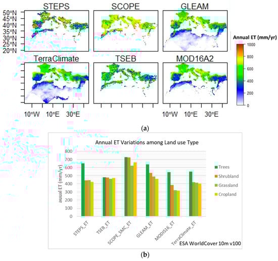
Figure 2.
(a) Total ET estimated from observed models [TSEB, SCOPE, STEPS] and reference products [GLEAM, MOD16, TerraClimate] over the Mediterranean region with their aggregated sum over major land cover types (b). Uncertainty is expected from the use of high-resolution land cover data (ESA—100 m WorldCover) for comparison.
The discrepancies in the annual pattern between models and products highlight the difference of approaches for ET estimation. Models like STEPS, SCOPE, TSEB, and MOD16A2 rely on LAI- and LST-driven schemes. These models perform well in capturing ET over cultivated semi-arid regions. However, models like GLEAM and TerraClimate take precipitation as the main input, which can lead to significant underestimations in the arid areas. The variability in ET in agroecosystems is largely influenced by vegetation characteristics like species composition and LAI []. For example, the spatial pattern of STEPS-ET closely resembles MOD16A2, particularly over southern Europe. This similarity is likely due to their use of a common LAI dataset and the Penman–Monteith approach. In contrast, TSEB and SCOPE, which incorporate LST, canopy temperature, and radiative responses, show greater spatial variability in ET across irrigated and non-irrigated zones.
This study represents the first combined regional-scale evaluation of these models (STEPS, SCOPE, TSEB) for ET estimation in the Mediterranean. The results provide some confidence in the ability of these models, particularly those incorporating LAI or LST, to capture ET over cultivated areas. However, limitations were also identified in areal coverage. Models relying solely on LAI exhibited missing values in arid regions of North Africa. Using precipitation as the main input in the case of GLEAM and TerraClimate also showed negligible ET estimates over irrigated zones.
Figure 2b highlights the differential responses of the models to different land cover types across the Mediterranean. TSEB’s estimates show minimal variation across land cover types at the 10 km resolution, likely due to pixel heterogeneity leading to uncertainty in canopy parameterization. This results in smaller gaps in ET between different land cover types. In contrast, SCOPE, due to its lack of explicit water limitations and its land cover-independent parameterization, produces higher ET values across all land cover types. However, LAI plays a dominant role in differentiating canopy response. Irrigated crops can also show higher ET than grasslands or shrublands, it is determined by SCOPE and TSEB. These models account for several surface characteristics, such as albedo, roughness, and vegetation properties, which influence energy balance calculations and can lead to higher ET estimates from irrigated crops. Other models show a larger gap of more than 100 mm in annual ET between forests and other land cover types, with a decreasing sequence of forest > shrubland > grassland > cropland. Forests typically have higher LAI, more complex canopies, and greater transpiration rates, leading to higher overall ET compared to other land covers. This finding aligns with observations from eddy covariance sites as well, where forests generally exhibit higher daily ET rates in the Mediterranean region. So, forests can show the highest cumulative ET in the Mediterranean region. Overall, the observed variations in annual ET patterns across land cover types highlight the need for accurate land cover parameterization and corresponding boundary conditions for reliable ET estimation.
3.2. Comparison of Seasonal Evapotranspiration Sums
Seasonal ET sums for 2019 from each model (STEPS, SCOPE, and TSEB) are also compared with reference datasets (MOD16, GLEAM, and TerraClimate). A spatial correlation was applied to examine the degree of agreement between the models and other products. The chosen period, March to November, captures the growing season and peak ET activity. Spatial variability among ET products is most prominent in summer (Figure 3a) when atmospheric water demand is typically high in the Mediterranean region. This reflects the models’ ability to capture the spatial dynamics of ET linked to seasonal variations in water demand. As expected, ET estimates are proportionally higher in summer, ranging from 0 to 350 mm in spring, from 150 to over 650 mm in summer, and declining to 0 to 150 mm in autumn. This seasonal pattern aligns well with daily ET trends reported in many Mediterranean site-scale measurements.
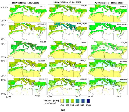
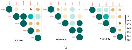
Figure 3.
(a) Seasonal evapotranspiration (ET) sums for the period March to November 2019 from STEPS, SCOPE, TSEB, MOD16A2, and GLEAM (b) refer to their corresponding correlation matrix. The highest correlations were observed between STEPS and GLEAM in spring and summer with TSEB in summer, and STEPS and GLEAM in autumn. Conversely, the lowest correlations were found in the case of SCOPE with other products. Seasonal demarcations for this comparison adhere to reference [].
During summer, when precipitation is minimal, GLEAM exhibited the lowest cumulative ET (<350 mm) compared to other models across all seasons. Other products showed some ET variability over the Balkans and France. Spatial autocorrelation analysis provided further insights into model agreement. STEPS showed a strong correlation with TSEB, MOD16A2, and GLEAM, with the strongest correlation observed between STEPS, TSEB, and GLEAM in summer. In contrast, SCOPE exhibited a generally lower correlation with other products, indicating that its spatial behavior is distinct. As expected, SCOPE also showed relatively high ET levels (>200–350 mm) over the Nile region, where ET is negligible in GLEAM’s estimates throughout the year (consistent with annual findings). On the other hand, STEPS, TSEB, and MOD16A2 exhibited good agreement across all seasons.
The likely reason for these spatial differences is how models are trained on closing water and energy balance when imbalances are caused by the radiation budget, latent heat flux, ground and sensible heat fluxes, or soil moisture dynamics. Additionally, differences in model parameterizations have influenced their outputs. The high correlation observed among STEPS, TSEB, and GLEAM in summer, and with MOD16A2 in spring, highlights their consistency and potential for intercomparison, particularly during the growing season.
3.3. Comparison of Total ET Estimates and Evaporative Stress Index over AOIs
Hourly potential evapotranspiration (PET), a derived dataset from the ASCE’s standardized reference ET model is used for countrywide atmospheric energy demand comparisons. Zonal statistics were applied to calculate the average precipitation (influx) and PET (outflux) for each country over a year. Figure 4 highlights the hydro-climatic disparities for the year 2019 in the Mediterranean countries. Precipitation is surplus in some countries (e.g., Montenegro, Bosnia, Albania, Italy, and Croatia) and deficits in others. This suggests favorable conditions for water availability, agriculture, and ecosystems in some southeast Mediterranean countries with precipitation surpluses. In contrast, the majority of Middle Eastern and North African (MENA) countries received less than 500 mm of annual rainfall, with the exceptions of Lebanon and Cyprus. Notably, Egypt is one of the driest countries, where PET reached above 1500 mm. In Egypt and other MENA countries (Libya, Tunisia, Algeria, Morocco) rainfall is low but evaporation demand is high, and agriculture is irrigation dependent. This makes water demand a dominant factor controlling water availability in the region. However, irrigation supplements the water deficit and allows agricultural activities to persist. The dependence on irrigation systems also highlights these regions’ fragility to changes in climate variability. Strong climate variability over southern Europe, Turkey, and the western Balkans has also been observed in recent years, affecting the water budget, and making their land use systems more vulnerable to water stress, which makes the two distinct climate clusters of hydrological imbalances more intense [], as shown in Figure 4 with a dotted borderline.
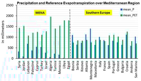
Figure 4.
The figure shows aggregated precipitation and potential ET in the year 2019 over different Mediterranean countries, retrieved from the annual total Precipitation from Soil Moisture to Rain (SM2rain) and Potential ET (PET) product from ERA5.
The comparison of ET across different land cover types of seven AOIs reveals more distinct model behaviors in arid regions. Figure 5a presents the area-averaged annual ET sums from all models across seven AOIs, in which SCOPE exhibits the highest values over croplands in Turkey, Morocco, Egypt, and the grasslands of Spain. In these areas with high PET near 1500 mm, indicating a high atmospheric water demand, GLEAM and TerraClimate show considerably lower ET there compared to other models, indicating their limitation in the arid cultivated regions. These model discrepancies highlight the importance of not relying on a single ET product for water use assessment. A complementary approach using multiple ET datasets is recommended for the arid regions in the Middle East and North Africa (MENA). However, differences in case of France, Italy, and the Balkans are less pronounced. Here, TSEB shows relatively low ET estimates over the forest ecosystems.
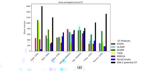
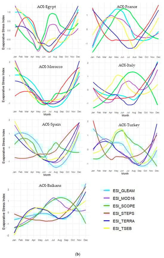
Figure 5.
(a) Area-averaged evapotranspiration (ET) from all products computed for specific areas of interest (AOIs) across various locations, representing different ecosystems to compare ET budget estimates from different products, revealing notable discrepancies among ET magnitudes. (b) Monthly time series of the Evaporative Stress Index (ESI) derived from ET products and ERA5-potential ET for assessing water stress in summer across various locations and ecosystems.
The Evaporative Stress Index (ESI) is employed to further assess how different ET products can influence the assessment of water stress (Figure 5b). An ESI value of −1.5 or lower indicates severe water stress, while +1.5 or higher suggests excessive soil moisture []. By comparing ESI derived from different models’ ET outputs, we observed variations in model performance over AOIs. For example, over croplands in Egypt, STEPS-GLEAM indicated water stress in June and July, whereas SCOPE-TSEB indicated earlier stress in May. It shows their effectiveness for irrigated croplands, assessing water demand earlier. Over grasslands in Spain, TSEB, MOD16A2, GLEAM, and TerraClimate showed a summer deficit, while STEPS and SCOPE did not, showing usability of the former over Spain. In the Balkan Forest, all models behaved entirely differently, making it challenging to decipher the uniform ET pattern of this region. The response of models over croplands in France was more consistent. STEPS, GLEAM, and TerraClimate, indicated similar trends, with only TerraClimate showing water stress in July, TSEB in August, and STEPS indicating stress throughout the summer. In contrast, all models agreed on water stress for croplands in Morocco during the same period, with SCOPE and TSEB again showing earlier stress as observed in Egypt. The overlapping responses by models in Morocco are likely due to the dominant role of high atmospheric demand and dry conditions. Ground ET measurements in Morocco would be valuable for verifying this uniform response by all models.
The following is inferred:
- Over Spain, TSEB, MOD16A2, GLEAM, and TerraClimate are showing consistent trends, giving robust signals of water stress in spring and summer, but this seasonal trend is absent in the case of STEPS and SCOPE, which means they need better parameterization for this climatic region, which is also observed in their ground validations over shrubland sites.
- Over Egypt, SCOPE’s and MOD16A2’s behaviors are comparable, whereas models that account for precipitation have collectively shown July as the most stressed month for Egypt (although not severe for STEPS, TSEB, GLEAM, and TerraClimate)
- Over France, similarity was found between SCOPE-GLEAM, TSEB-MOD16A2, and between STEPS-TerraClimate. These models also showed good accuracy for forest sites.
- A robust agreement among all models was observed over croplands in Morocco, which may be due to the dominance of the crop ecosystem or the strong influence of atmospheric demand and dry conditions in summer.
Based on these results, the feasibility of using ensemble ET outputs from these models is likely supported for croplands in Morocco. ET estimation remains challenging in the Balkans, where irregular precipitation patterns further complicate the determination of ET trends with the least definite ET seasonality (Figure 4). This evaluation highlights the highly diverse nature of ET across the Mediterranean region, suggesting that a single approach may not be optimal for modeling ET flux, particularly in regions where both energy and water limitations coexist. A pragmatic approach is needed with a combination of methods, necessitating careful consideration of climate clustering or regional segregation during model parameterization (as in Figure 4).
Unlike many studies that focus on broad comparisons of annual and monthly ET estimates, this study provides deeper insights into modeled ET at sub-regional, seasonal, and ecosystem scales through its application to water stress assessment via evaporative stress index. Our findings suggest that modeled ET may be unreliable for specific regions, such as the Balkans and Turkey. Significant improvements in model parameterizations are needed in these areas. Given the limited ground observations of ET in North Africa and the eastern Mediterranean region, model validation over this region remains understudied, particularly for desert and oasis ecosystems []. We need ongoing model refinement, validation, and integration with ground-based observations to address these limitations and improve ET estimates across the region.
3.4. Daily Time-Series: Modeled ET vs. Eddy Covariance ET
To assess the accuracy of the models on the ground, daily time series data for 2019 were compared with eddy covariance observations from 17 sites across southern Europe and 1 site in Israel (IL-Yat). These sites encompass a diverse range of ecosystems, including evergreen needle forests, deciduous boreal forests, evergreen boreal forests, croplands, grasslands, shrublands, and savannahs covering mostly ecosystems in southern Europe.
The results have shown daily ET varies across land cover types. Forests in France and Italy exhibited the highest daily ET (>6 mm/day), followed by croplands (<6 mm/day), and shrublands/savannahs (around 4 mm/day). This trend in higher ET in Mediterranean forests was consistent across some models (mainly STEPS) (Figure 3b). However, seasonal ET patterns differed among models across sites. For instance, STEPS and SCOPE overestimated summer ET in Spanish shrublands, while GLEAM and TSEB captured the right ET pattern observed there. In contrast, all models agreed on seasonal patterns in some Italian and French croplands and forests. Discrepancies in boreal forests and savannahs highlight the need for improvements in capturing the phenological response of these ecosystems (e.g., STEPS, SCOPE, TSEB).
Forest and grassland sites generally showed the strongest agreement between modeled and eddy covariance (EC) ET observations (r2 = 0.6–0.8), with low root mean square error (RMSE) and mean bias error (MBE) (Figure 6). IT_MBo exhibited the highest coefficient of determination (r2) scores, indicating strong agreement between modeled and ET observations in the range of 0.6–0.8. Their corresponding root mean square error (RMSE) and mean bias error (MBE) were also low (Figure 6), showing the high accuracy of these models in these two ecosystems (forests and grasslands). SCOPE and STEPS also showed good agreement in some forest, grassland, and cropland sites, while GLEAM performed best in shrublands. GLEAM, along with other sites, showed the highest congruence in shrubland sites (ES_LM1, ES_LM2, and ES_LMa), whereas only TSEB showed high congruence afterward.
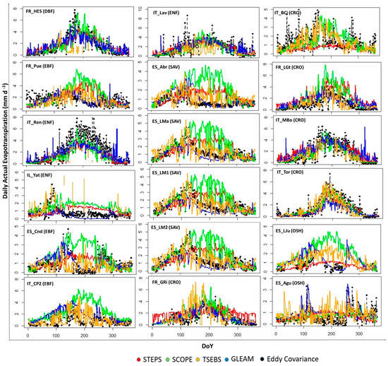
Figure 6.
Daily time series of ET derived from models [STEPS, SCOPE, TSEB, GLEAM] and their comparison with daily observations from 18 eddy covariance sites presenting four ecosystems (forest, savannah, shrubland, and cropland) of the Mediterranean countries.
Five out of eighteen sites (mostly in France and Italy) showed significant agreement with both STEPS and SCOPE models (FR_HES, IT_Ren, FR_LGt, IT_MBo, and IT_Tor) (Figure 7). However, several sites exhibited lower accuracies. The Israeli forest (IL_Yat), Italian cropland (IT_BCi), and Spanish shrublands (ES_LJu and ES_Agu) showed lower agreement with modeled ET. Similarly, all models showed poor performance in evergreen boreal forest sites (ES_Cnd, FR_Pue, and IT_CP2), suggesting a need for improved model parameterization for boreal ecosystems, which are prone to wildfire in the Mediterranean region in the context of heat waves and water stress.
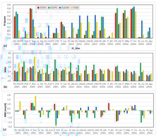
Figure 7.
Displays plots of the r-square coefficient of determination, (a) root mean square error RMSE (b), and (c) mean bias error (MBE) of all models [STEPS, SCOPE, TSEB, and GLEAM] explaining the relative performance of these models in Mediterranean ecosystems.
In summary, SCOPE demonstrates good performance with grasslands, GLEAM shows better in savannahs, and STEPS shows good performance in certain forest and crop sites. The performance of these products was checked with both unadjusted fluxes’ original ET and corrected fluxes for energy balance closure (ETebc); accuracy results were the same. Diego Salazar et al., 2022, also noticed, when evaluating with the original unadjusted ET flux, that GLEAM and ALEXI showed the highest coefficient of determination (r2), smallest percent bias (PBIAS), and best root mean square error (RMSE) with unadjusted ET [].
Weak agreement with other EC sites may stem from seasonal fluctuations in meteorological, soil, and land conditions, as well as the limitations of some models in capturing heterogeneity in ecosystems. Some models cannot perform well in heterogeneous ecosystems. This limitation was noticed by Burchard-Levine et al. (2020) first in TSEB, and they recommended seasonal adaptations of TSEB for a dominant vegetation cover for a given period to accurately estimate ET at a large spatial scale []. This validation lacks ground-based ET data over North Africa, limiting our ability to validate model responses over irrigated croplands in countries like Egypt, Morocco, and other North African countries. These regions exhibit significant seasonal variability in irrigated ET as observed in the ET magnitude and spatial patterns above, ground validation is major limitation for building confidence of using these models.
4. Discussion
The presented study highlights the complexities and uncertainties surrounding ET estimation in the Mediterranean region. Different models rely on distinct approaches. Some, like MOD16A2 and TSEB, focus solely on the energy balance approach, while others like STEPS and GLEAM couple energy and water balance approaches. This inherent bias can lead to contrasting ET patterns even with identical meteorological data, as we used for our models. This study delves deeper into how each model’s underlying assumptions influence ET calculations across diverse landscapes in the Mediterranean region. The lesson learned is that the choice of model should be driven by the specific objective. Short-term crop water requirement estimations benefit from process-based models that incorporate a wider range of factors beyond just climate and vegetation cover. Conversely, long-term and seasonal assessments might find energy balance models more suitable [,]. Traditional approaches that do not consider topographic and radiative influences on ET also surpass water or energy limits due to differences in the available energy −−should not be used for arid regions. As observed in the case of the TerraClimate and GLEAM estimates over Egypt, it is highly recommended to use near-surface air temperature with precipitation in dry ecosystems to derive patterns of ET [].
ET can have a lot of uncertainties due to the misinterpretation of the models, types of input, differences in scale and temporal/spatial resolution, and data coverage. This study rightly emphasizes the need for the careful evaluation of models before applying their output in critical areas like budget estimation, water productivity assessment, water use assessments, etc. []. A rigorous comparison of various models’ accuracy with established ground-truth data or other reliable sources is crucial. We identified the strengths and weaknesses of these models across diverse Mediterranean ecosystems to guide researchers in selecting the most appropriate tool for each specific scenario. Revising STEPS and SCOPE model parameterization is recommended for dry ecosystems, i.e., rainfed, shrublands, savannahs, etc. The comparison showed a contrasting difference in ET patterns: the annual and seasonal patterns showed that SCOPE’s response was closer to potential ET across the region, and STEPS is more aligned with MOD16A2-GLEAM compared to SCOPE-TSEB. A fundamental difference in the modeled ET estimates stems from their underlying approach: some are driven solely by the energy balance approach (such as MOD16A2 and TSEB) [,], radiative forcing and energy balancing (SCOPE), while others couple energy and water balance approaches (like STEPS and GLEAM). This disparity might have led to different patterns over southern Europe and MENA, and even the use of common meteorological forcings has no effect. Surface condition parameters (e.g., LST, LAI, LULC) have significantly influenced ET calculations. LST and LAI, being major components of these models, are not temporally consistent with climatic parameters, and this is another limitation. This might have also influenced the accuracy of our daily ET. Similar behavior is observed in the comparison of Landflux, GLDAS, GLEAM, and ERA-Interim, which all failed to capture evaporative flux over irrigated croplands, so high-resolution LST and LAI forcings were suggested []. In addition, some recent products, i.e., CSIRO MODIS ReScaled EvapoTranspiration (CMRSET), SSEBop, and WaPOR are found as less biased than MOD16A2 and GLEAM with an improved land surface parameterization for dry ecosystems. Integrating fractional vegetation cover and climatic water deficit into algorithms can also reduce model uncertainties [,].
The choice of variables in each model affects how they capture and represent the complex processes involved in ET, which affects the accuracy of ET estimates []. LAI is the most influential parameter in our models, as in SCOPE and STEPS, it determines photosynthetic foliage and influences the interception of rainfall and the subsequent evaporation from the vegetation canopy. In TSEB, it determines the fraction of incoming solar radiation intercepted by the vegetation canopy. Other models like GLEAM emphasize the role of vegetation dynamics and precipitation in driving ET by relying on VOD and precipitation, their comparison was challenging due to differences in input data and estimation algorithms; however, this revealed that accuracy can be increased over the region by improving inputs and modifying parameters for dry ecosystems. The area-specific parameterization can improve ET models’ performance in a given area or basin [,]. The “one-size-fits-all” approach for model parameters might not be optimal for the entire Mediterranean with its diverse climate clustering. Future research should prioritize area/climate-specific parameterization. This involves customizing model parameters based on unique regional conditions of soil types, vegetation characteristics, and prevailing climatic patterns. Such fine-tuning can significantly enhance model performance in specific regions within the Mediterranean basin considering the extremely arid and humid conditions. Future research should focus on parameterizing and training models to handle these extremes effectively. This is particularly critical given the increasing atmospheric demand leading to flash droughts and floods across the region.
The assimilation of high-resolution remote sensing data with advanced modeling techniques holds immense potential for generating robust ET estimates. By addressing these areas, we can ensure a more robust scientific foundation for ET estimation in the Mediterranean. This will not only improve the accuracy of water resource management but also enhance our understanding of the complex hydrological processes within this diverse and ecologically sensitive region. This inter-comparison somehow facilitated comprehending the shortcomings of each model, and how they can be modified for their future adaptation to the heterogeneous Mediterranean region.
5. Conclusions
While many studies broadly compare annual and monthly ET estimates, this study provides deeper insights into modeled ET at the sub-regional, seasonal, and ecosystem scales with its implication in seasonal stress prediction. Errors in ET estimates can have profound implications for regional water budget assessments and evaluations of agro-ecological drought risk. Therefore, it is imperative to continue refining model parameterization and enhancing the accuracy of ET simulations. Comparing models like STEPS, SCOPE, and TSEB reveals inconsistencies in their ET estimations for similar meteorological conditions. This exposes inherent biases within each model’s algorithms and assumptions for Mediterranean conditions. These inter-model comparisons revealed the significant influence of factors like LST, LAI, and subsurface hydrology on regional-scale ET calculations. This knowledge can help improve datasets on these factors during model improvement and parameter refining.
Key insights are as follows:
- STEPS encountered challenges in effectively modulating the seasonality of ET over different ecosystems. SCOPE gave higher evapotranspiration (ET) estimates during summer, and TSEB yielded lower ET estimates over forest ecosystems.
- TSEB showed larger uncertainty in its current parameterization routine, particularly when applied at a scale of 10 km. However, studies have shown that its less than 15% discrepancies in validation against ground observations when used at high resolution. To enhance its applicability across the large Mediterranean region, a seasonal adaptation of the model while considering dominant vegetation cover for a given period is recommended [,], and more specific vegetation parameterization, especially for forests, is required.
- GLEAM could not perform well over irrigated Nile Egypt. GLEAM’s limitations in irrigated areas suggest the need for an improved representation of crop phenology. However, it showed good results in semi-arid ecosystems of Spain and France, with potential use of microwave satellite-based products.
- STEPS showed some spatial similarity with existing global datasets and produced satisfactory simulation results, over some forest and crop sites. However, for large-scale applications, it requires extensive sub-regional scale parameterization, as this generic parameterization has yielded unreliable results in some locations.
- The evaporative stress index across different regions has shown robust agreement and reliability among these models in some areas, i.e., Morocco, Spain, and Egypt, where ground data were missing but the absence of significant trends over Italy, Balkans, and Turkey indicates the need for region-specific model calibration and validation for all models.
None of the models could holistically capture ET patterns across the entire region, and each has limitations and weaknesses in particular climates and ecosystems. This comparison, however, indicates areas of improvement in these models. Further investigation into model physics and forcing errors can enhance the overall robustness of ET simulations. Generic parameterizations used in some models (e.g., STEPS, TSEB, and SCOPE) can lead to unreliable results in certain locations. We should prioritize creating parameter sets tailored to specific regions and ecosystems within the Mediterranean. This will lead to more accurate model representations of local ET dynamics. Integrating high-resolution remote sensing data using advanced data assimilation offers significant potential for improving model accuracy. Tuning models for accurately representing extremely humid and arid environments within the Mediterranean will enhance their applicability in water management and environmental planning across the Middle East, North Africa, and Scandinavian regions.
Author Contributions
Conceptualization, Z.U. and A.G.; methodology, Z.U., A.G., E.P. and V.B.-L.; software, Z.U., A.G., E.P., C.V.d.T. and V.B.-L.; data curation, Z.U., A.G. and E.P.; writing—original draft preparation, Z.U.; writing—review and editing, E.P., V.B.-L., B.L., C.V.d.T. and M.M.; visualization, Z.U.; supervision, M.M., A.G., B.L. and C.V.d.T. All authors have read and agreed to the published version of the manuscript.
Funding
This research is funded by (1) the CGIAR Initiative on Climate Resilience, ClimBeR and (2) Regional Water Harvesting Potential Mapping Project under SIDA and FAO.
Institutional Review Board Statement
Not applicable.
Informed Consent Statement
Not applicable.
Data Availability Statement
Data will be shared publicly.
Acknowledgments
We acknowledge the doctoral scholarship awarded to Z.U. by the Department of Innovation in Biology, Agri-food, and Forest Systems (DIBAF) at the University of Tuscia, Viterbo, Italy, as well as the short scientific mission grant provided by the SENSECO COST Action program (CA17134). We are grateful to the CGIAR Initiatives on [1] Climate Resilience (ClimBeR) and [2] Fragility to Resilience in Central and West Asia and North Africa
(F2R-CWANA), and the International Center for Agricultural Research in the Dry Areas (ICARDA) for the support and also for providing the STEPS model. The authors extend thanks to the Faculty of Geoinformation Science and Earth Observation ITC, Netherlands, and UNIMOL DiBT Forestry Lab@Pesche for their support. We acknowledge scientific data providers, i.e., Copernicus Climate Change Service (C3S) Climate Data Store (CDS) for meteorological forcing datasets, NASA’s Land Processes Distributed Active Archive Center (LP DAAC) for MOD16A2.006 ET product, ICOS-DIBAF UNITUS for the LE Flux database, the Geospatial Information Authority of Japan, Chiba University, and their collaborating organizations for sharing the land cover database, and ISRIC–EU-H2020 for providing free access to their latest release (May 2020) of SoilGrids Information.
Conflicts of Interest
The authors declare no conflicts of interest.
References
- Krishna, P.R. Evapotranspiration and agriculture. A review. Agric. Rev. 2019, 40, 1–11. [Google Scholar]
- Urdiales-Flores, D.; Zittis, G.; Hadjinicolaou, P.; Osipov, S.; Klingmüller, K.; Mihalopoulos, N.; Kanakidou, M.; Economou, T.; Lelieveld, J. Drivers of accelerated warming in Mediterranean climate-type regions. Npj Clim. Atmos. Sci. 2023, 6, 97. [Google Scholar] [CrossRef]
- Brown, P. Basics of Evaporation and Evapotranspiration; College of Agriculture and Life Sciences, University of Arizona: Tucson, AZ, USA, 2014. [Google Scholar]
- Unnisa, Z.; Govind, A.; Lasserre, B.; Marchetti, M. Water Balance Trends along Climatic Variations in the Mediterranean Basin over the Past Decades. Water 2023, 15, 1889. [Google Scholar] [CrossRef]
- Boulet, G.; Jarlan, L.; Olioso, A.; Nieto, H. Chapter 2—Evapotranspiration in the Mediterranean region. In Water Resources in the Mediterranean Region; Zribi, M., Brocca, L., Tramblay, Y., Molle, F., Eds.; Elsevier: Amsterdam, The Netherlands, 2020; pp. 23–49. ISBN 978-0-12-818086-0. [Google Scholar]
- Katerji, N.; Campi, P.; Mastrorilli, M. Productivity, evapotranspiration, and water use efficiency of corn and tomato crops simulated by AquaCrop under contrasting water stress conditions in the Mediterranean region. Agric. Water Manag. 2013, 130, 14–26. [Google Scholar] [CrossRef]
- Wang, K.; Wang, P.; Li, Z.; Cribb, M.; Sparrow, M. A simple method to estimate actual evapotranspiration from a combination of net radiation, vegetation index and temperature. J. Geophys. Res. 2007, 112, D15107. [Google Scholar] [CrossRef]
- Anderson, M.; Kustas, W. Thermal remote sensing of drought and evapotranspiration. Eos Trans. Am. Geophys. Union 2008, 89, 233–234. [Google Scholar] [CrossRef]
- Ubing, D.S. Solar and net radiation, available energy and its influence on evapotranspiration from grass. Neth. J. Agric. Sci. 1961, 9, 81–93. [Google Scholar]
- Jensen, M.E. Empirical methods of estimating or predicting evapotranspiration using radiation. In Proceedings of the ASAE Conference Evapotranspiration and Its Role in Water Resources Management, Chicago, IL, USA, 5–6 December 1966; pp. 49–53, 64. [Google Scholar]
- Glenn, E.P.; Neale, C.M.; Hunsaker, D.J.; Nagler, P.L. Vegetation index-based crop coefficients to estimate evapotranspiration by remote sensing in agricultural and natural ecosystems. Hydrol. Process. 2011, 25, 4050–4062. [Google Scholar] [CrossRef]
- Allen, R.G.; Pereira, L.S.; Smith, M.; Raes, D.; Wright, J.L. FAO-56 dual crop coefficient method for estimating evaporation from soil and application extensions. J. Irrig. Drain. Eng. 2005, 131, 2–13. [Google Scholar] [CrossRef]
- Miao, Q.; Rosa, R.D.; Shi, H.; Paredes, P.; Zhu, L.; Dai, J.; Gonçalves, J.M.; Pereira, L.S. Modeling water use, transpiration and soil evaporation of spring wheat–maize and spring wheat–sunflower relay intercropping using the dual crop coefficient approach. Agric. Water Manag. 2016, 165, 211–229. [Google Scholar] [CrossRef]
- Nisa, Z.; Govind, A.; Marchetti, M.; Lasserre, B. A review of crop water productivity in the Mediterranean Basin under changing climate: Wheat and barley as test cases. Irrig. Drain. 2022, 71, 51–70. [Google Scholar] [CrossRef]
- Allen, R.G.; Morton, C.; Kamble, B.; Kilic, A.; Huntington, J.; Thau, D.; Gorelick, N.; Erickson, T.; Moore, R.; Trezza, R. EEFlux: A Landsat-based evapotranspiration mapping tool on the Google Earth Engine. In Proceedings of the 2015 ASABE/IA Irrigation Symposium, Long Beach, CA, USA, 10–12 November 2015; pp. 1–11. [Google Scholar]
- Bhattarai, N.; Wagle, P. Recent Advances in Remote Sensing of Evapotranspiration. Remote Sens. 2021, 13, 4260. [Google Scholar] [CrossRef]
- Gallego-Elvira, B.; Olioso, A.; Mira, M.; Reyes-Castillo, S.; Boulet, G.; Marloie, O.; Garrigues, S.; Courault, D.; Weiss, M.; Chauvelon, P. EVASPA (EVapotranspiration assessment from SPAce) tool: An overview. Proc. Environ. Sci. 2013, 19, 303–310. [Google Scholar] [CrossRef]
- Holmes, T.R.; Hain, C.R.; Crow, W.T.; Anderson, M.C.; Kustas, W.P. Microwave implementation of two-source energy balance approach for estimating evapotranspiration. Hydrol. Earth Syst. Sci. 2018, 22, 1351–1369. [Google Scholar] [CrossRef] [PubMed]
- Carpintero, E.; Anderson, M.C.; Andreu, A.; Hain, C.; Gao, F.; Kustas, W.P.; González-Dugo, M.P. Estimating Evapotranspiration of Mediterranean Oak Savanna at Multiple Temporal and Spatial Resolutions. Implications for Water Resources Management. Remote Sens. 2021, 13, 3701. [Google Scholar] [CrossRef]
- Melton, F.S.; Huntington, J.; Grimm, R.; Herring, J.; Hall, M.; Rollison, D.; Erickson, T.; Allen, R.; Anderson, M.; Fisher, J.B.; et al. OpenET: Filling a critical data gap in water management for the western United States. JAWRA J. Am. Water Resour. Assoc. 2022, 58, 971–994. [Google Scholar] [CrossRef]
- De Oliveira Ferreira Silva, C.; Lilla Manzione, R.; Albuquerque Filho, J.L. Large-scale spatial modeling of crop coefficient and biomass production in agroecosystems in southeast Brazil. Horticulturae 2018, 4, 44. [Google Scholar] [CrossRef]
- Pereira, L.S.; Paredes, P.; Melton, F.; Johnson, L.; Wang, T.; López-Urrea, R.; Cancela, J.J.; Allen, R.G. Prediction of crop coefficients from fraction of ground cover and height. Background and validation using ground and remote sensing data. Agric. Water Manag. 2020, 241, 106197. [Google Scholar] [CrossRef]
- Chirouze, J.; Boulet, G.; Jarlan, L.; Fieuzal, R.; Rodriguez, J.C.; Ezzahar, J.; Er-Raki, S.; Bigeard, G.; Merlin, O.; Garatuza-Payan, J. Intercomparison of four remote-sensing-based energy balance methods to retrieve surface evapotranspiration and water stress of irrigated fields in semi-arid climate. Hydrol. Earth Syst. Sci. 2014, 18, 1165–1188. [Google Scholar] [CrossRef]
- Gonzalez-Dugo, M.; Neale, C.; Mateos, L.; Kustas, W.; Prueger, J.; Anderson, M.; Li, F. A comparison of operational remote sensing-based models for estimating crop evapotranspiration. Agric. For. Meteorol. 2009, 149, 1843–1853. [Google Scholar] [CrossRef]
- Song, L.; Kustas, W.P.; Liu, S.; Colaizzi, P.D.; Nieto, H.; Xu, Z.; Ma, Y.; Li, M.; Xu, T.; Agam, N. Applications of a thermal-based two-source energy balance model using Priestley-Taylor approach for surface temperature partitioning under advective conditions. J. Hydrol. 2016, 540, 574–587. [Google Scholar] [CrossRef]
- Kirnak, H. A Comparison Between Deterministic and Stochastic Evapotranspiration Models for Container Grown Acer Rubrum. Int. J. Agric. Nat. Sci. 2014, 7, 33–38. [Google Scholar]
- Tang, R.; Li, Z.L.; Tang, B.; Wu, H. Interpretation of surface temperature/vegetation index space for evapotranspiration estimation from SVAT modeling. In Proceedings of the 2015 IEEE International Geoscience and Remote Sensing Symposium (IGARSS) (2028–2030), Milan, Italy, 26–31 July 2015; IEEE: Piscataway, NJ, USA. [Google Scholar] [CrossRef]
- Doung Vo, N.; Gourbesville, P. Application of deterministic distributed hydrological model for large catchment: A case study at Vu Gia Thu Bon catchment, Vietnam. J. Hydrol. 2016, 18, 885–904. [Google Scholar]
- Olchev, A.; Ibrom, A.; Priess, J.; Erasmi, S.; Leemhuis, C.; Twele, A.; Radler, K.; Kreilein, H.; Panferov, O.; Gravenhorst, G. Effects of land-use changes on evapotranspiration of tropical rain forest margin area in Central Sulawesi (Indonesia): Modelling study with a regional SVAT model. Ecol. Modell. 2008, 212, 131–137. [Google Scholar] [CrossRef]
- Olioso, A.; Rivalland, V.; Faivre, R.; Weiss, M.; Demarty, J.; Wassenaar, T.; Baret, F.; Cardot, H.; Rossello, P.; Jacob, F. Monitoring evapotranspiration over the alpilles test site by introducing remote sensing data at various spatial resolutions into a dynamic SVAT model. In AIP Conference Proceedings; American Institute of Physics: College Park, MD, USA, 2006; Volume 852, pp. 234–241. [Google Scholar]
- Govind, A.; Cowling, S.; Kumari, J.; Rajan, N.; Al-Yaari, A. Distributed modeling of ecohydrological processes at high spatial resolution over a landscape having patches of managed forest stands and crop fields in SW Europe. Ecol. Model. 2015, 297, 126–140. [Google Scholar] [CrossRef]
- Yang, P.; Prikaziuk, E.; Verhoef, W.; van Der Tol, C. SCOPE 2.0: A model to simulate vegetated land surface fluxes and satellite signals. Geosci. Model Dev. 2021, 14, 4697–4712. [Google Scholar] [CrossRef]
- Bigeard, G.; Coudert, B.; Chirouze, J.; Er-Raki, S.; Boulet, G.; Ceschia, E.; Jarlan, L. Ability of a soil–vegetation–atmosphere transfer model and a two-source energy balance model to predict evapotranspiration for several crops and climate conditions. Hydrol. Earth Syst. Sci. 2019, 23, 5033–5058. [Google Scholar] [CrossRef]
- Singer, M.B.; Asfaw, D.T.; Rosolem, R.; Cuthbert, M.O.; Miralles, D.G.; MacLeod, D.; Quichimbo, E.A.; Michaelides, K. Hourly potential evapotranspiration at 0.1 resolution for the global land surface from 1981-present. Sci. Data 2021, 8, 224. [Google Scholar] [CrossRef] [PubMed]
- Prikaziuk, E.; Yang, P.; van der Tol, C. Google Earth Engine Sentinel-3 OLCI Level-1 Dataset Deviates from the Original Data: Causes and Consequences. Remote Sens. 2021, 13, 1098. [Google Scholar] [CrossRef]
- Guzinski, R.; Nieto, H.; Sandholt, I.; Karamitilios, G. Modelling high-resolution actual evapotranspiration through Sentinel-2 and Sentinel-3 data fusion. Remote Sens. 2020, 12, 1433. [Google Scholar] [CrossRef]
- Ciabatta, L.; Massari, C.; Brocca, L.; Gruber, A.; Reimer, C.; Hahn, S.; Paulik, C.; Dorigo, W.; Kidd, R.; Wagner, W. SM2RAIN-CCI: A new global long-term rainfall data set derived from ESA CCI soil moisture. Earth Syst. Sci. Data 2018, 10, 267–280. [Google Scholar] [CrossRef]
- Prikaziuk, E.; Migliavacca, M.; Su, Z.B.; van der Tol, C. Simulation of ecosystem fluxes with the SCOPE model: Sensitivity to parametrization and evaluation with flux tower observations. Remote Sens. Environ. 2023, 284, 113324. [Google Scholar] [CrossRef]
- Jacquemoud, S.; Baret, F. PROSPECT: A model of leaf optical properties spectra. Remote Sens. Environ. 1990, 34, 75–91. [Google Scholar] [CrossRef]
- Van der Tol, C.; Verhoef, W.; Timmermans, J.; Verhoef, A.; Su, Z. An integrated model of soil-canopy spectral radiances, photosynthesis, fluorescence, temperature and energy balance. Biogeosciences 2009, 6, 3109–3129. [Google Scholar] [CrossRef]
- Guzinski, R.; Anderson, M.C.; Kustas, W.P.; Nieto, H.; Sandholt, I. Using a thermal-based two source energy balance model with time-differencing to estimate surface energy fluxes with day-night MODIS observations. Hydrol. Earth Syst. Sci. 2013, 17, 2809–2825. [Google Scholar] [CrossRef]
- Guzinski, R.; Nieto, H.; Sánchez, J.M.; López-Urrea, R.; Boujnah, D.M.; Boulet, G. Utility of Copernicus-based inputs for actual evapotranspiration modeling in support of sustainable water use in agriculture. IEEE J. Sel. Top. Appl. Earth Obs. Remote Sens. 2021, 14, 11466–11484. [Google Scholar] [CrossRef]
- Mu, Q.; Heinsch, F.A.; Zhao, M.; Running, S.W. Development of a global evapotranspiration algorithm based on MODIS and global meteorology data. Remote Sens. Environ. 2007, 111, 519–536. [Google Scholar] [CrossRef]
- Miralles, D.G.; Holmes, T.R.H.; De Jeu, R.A.M.; Gash, J.H.; Meesters, A.G.C.A.; Dolman, A.J. Global land-surface evaporation estimated from satellite-based observations. Hydrol. Earth Syst. Sci. 2011, 15, 453–469. [Google Scholar] [CrossRef]
- Abatzoglou, J.T.; Dobrowski, S.Z.; Parks, S.A.; Hegewisch, K.C. TerraClimate, a high-resolution global dataset of monthly climate and climatic water balance from 1958–2015. Sci. Data 2018, 5, 170191. [Google Scholar] [CrossRef]
- Kotsias, G.; Lolis, C.J.; Hatzianastassiou, N.; Lionello, P.; Bartzokas, A. An objective definition of seasons for the Mediterranean region. Int. J. Climatol. 2021, 41, E1889–E1905. [Google Scholar] [CrossRef]
- Khalil, A.A.; Essa, Y.H.; Abdel-Wahab, M.M. Evapotranspiration mapping over Egypt using MODIS/Terra satellite data. Int. J. Adv. Res. 2015, 15, 512–522. [Google Scholar]
- Zeng, Z.; Piao, S.; Li, L.Z.; Wang, T.; Ciais, P.; Lian, X.; Yang, Y.; Mao, J.; Shi, X.; Myneni, R.B. Impact of Earth greening on the terrestrial water cycle. J. Clim. 2018, 31, 2633–2650. [Google Scholar] [CrossRef]
- Anderson, M.C.; Hain, C.; Wardlow, B.; Pimstein, A.; Mecikalski, J.; Kustas, W. A thermal-based evaporative stress index for monitoring surface moisture depletion. In Remote Sensing of Drought: Innovative Monitoring Approaches; CRC Press/Taylor & Francis: Boca Raton, FL, USA, 2012; pp. 145–167. [Google Scholar]
- Salazar-Martínez, D.; Holwerda, F.; Holmes, T.R.; Yépez, E.A.; Hain, C.R.; Alvarado-Barrientos, S.; Ángeles-Pérez, G.; Arredondo-Moreno, T.; Delgado-Balbuena, J.; Figueroa-Espinoza, B. Evaluation of remote sensing-based evapotranspiration products at low-latitude eddy covariance sites. J. Hydrol. 2022, 610, 127786. [Google Scholar] [CrossRef]
- Burchard-Levine, V.; Nieto, H.; Riaño, D.; Migliavacca, M.; El-Madany, T.S.; Perez-Priego, O.; Carrara, A.; Martín, M.P. Seasonal adaptation of the thermal-based two-source energy balance model for estimating evapotranspiration in a semiarid tree-grass ecosystem. Remote Sens. 2020, 12, 904. [Google Scholar] [CrossRef]
- Qian, T.; Dai, A.; Trenberth, K.E.; Oleson, K.W. Simulation of global land surface conditions from 1948 to 2004. Part I: Forcing data and evaluations. J. Hydrometeorol. 2006, 7, 953–975. [Google Scholar] [CrossRef]
- Parajuli, P.B.; Risal, A.; Ouyang, Y.; Thompson, A. Comparison of SWAT and MODIS evapotranspiration data for multiple timescales. Hydrology 2022, 9, 103. [Google Scholar] [CrossRef]
- Stisen, S.; Soltani, M.; Mendiguren, G.; Langkilde, H.; Garcia, M.; Koch, J. Spatial patterns in actual evapotranspiration climatologies for Europe. Remote Sens. 2021, 13, 2410. [Google Scholar] [CrossRef]
- Ojeda, M.G.V.; Rosa-Cánovas, J.J.; Romero-Jimenez, E.; Yeste, P.; Gamiz-Fortis, S.R.; Castro-Diez, Y.; Esteban-Parra, M.J. The role of surface evapotranspiration in regional climate modelling: Evaluation and near-term future changes. Atmos. Res. 2020, 237, 104867. [Google Scholar] [CrossRef]
- Dile, Y.T.; Ayana, E.K.; Worqlul, A.W.; Xie, H.; Srinivasan, R.; Lefore, N.; You, L.; Clarke, N. Evaluating satellite-based evapotranspiration estimates for hydrological applications in data-scarce regions: A case in Ethiopia. Sci. Total Environ. 2020, 743, 140702. [Google Scholar] [CrossRef]
- Chen, X.; Su, Z.; Ma, Y.; Trigo, I.; Gentine, P. Remote sensing of global daily evapotranspiration based on a surface energy balance method and reanalysis data. J. Geophys. Res. Atmos. 2021, 126, e2020JD032873. [Google Scholar] [CrossRef]
- Wu, B.; Zhu, W.; Yan, N.; Xing, Q.; Xu, J.; Ma, Z.; Wang, L. Regional actual evapotranspiration estimation with land and meteorological variables derived from multi-source satellite data. Remote Sens. 2020, 12, 332. [Google Scholar] [CrossRef]
- Blatchford, M.L.; Mannaerts, C.M.; Zeng, Y.; Nouri, H.; Karimi, P. Status of accuracy in remotely sensed and in-situ agricultural water productivity estimates: A review. Remote Sens. Environ. 2019, 234, 111413. [Google Scholar] [CrossRef]
- Long, D.; Longuevergne, L.; Scanlon, B.R. Uncertainty in evapotranspiration from land surface modeling, remote sensing, and GRACE satellites. Water Resour. Res. 2014, 50, 1131–1151. [Google Scholar] [CrossRef]
- Kustas, W.P.; Alfieri, J.G.; Nieto, H.; Wilson, T.G.; Gao, F.; Anderson, M.C. Utility of the two-source energy balance (TSEB) model in vine and interrow flux partitioning over the growing season. Irrig. Sci. 2019, 37, 375–388. [Google Scholar] [CrossRef]
- Sanchez, J.M.; López-Urrea, R.; Valentín, F.; Caselles, V.; Galve, J.M. Lysimeter assessment of the Simplified Two-Source Energy Balance model and eddy covariance system to estimate vineyard evapotranspiration. Agric. For. Meteorol. 2019, 274, 172–183. [Google Scholar] [CrossRef]
- Burchard-Levine, V.; Nieto, H.; Riaño, D.; Migliavacca, M.; El-Madany, T.S.; Guzinski, R.; Carrara, A.; Martín, M.P. The effect of pixel heterogeneity for remote sensing based retrievals of evapotranspiration in a semi-arid tree-grass ecosystem. Remote Sens. Environ. 2021, 260, 112440. [Google Scholar] [CrossRef]
Disclaimer/Publisher’s Note: The statements, opinions and data contained in all publications are solely those of the individual author(s) and contributor(s) and not of MDPI and/or the editor(s). MDPI and/or the editor(s) disclaim responsibility for any injury to people or property resulting from any ideas, methods, instructions or products referred to in the content. |
© 2024 by the authors. Licensee MDPI, Basel, Switzerland. This article is an open access article distributed under the terms and conditions of the Creative Commons Attribution (CC BY) license (https://creativecommons.org/licenses/by/4.0/).