Abstract
In this work, the lumped model of Rogowski coils is briefly reviewed to illustrate that the reduction in stray capacitance expands the bandwidth and improves the high-frequency performance. Then, a network model as well as explicit formulas for the stray capacitance of Rogowski coils are established, and the influence of geometrical parameters of the skeletons on the stray capacitance is investigated. It is found that the stray capacitance of Rogowski coils is approximately proportional to the perimeter of the skeleton cross-section. Based on the above discussion, optimization of the shape of the skeleton cross-section, aiming at minimizing the perimeter without affecting the magnetic flux and mutual inductance of the coils, is carried out. The widely adopted circular and rectangular cross-sections are discussed first. Then, the cross-section of an arbitrary smooth and convex shape is optimized by solving a constrained variational problem, leading to an explicit equation for the optimal skeleton cross-section of Rogowski coils. Numerical results demonstrate that, compared with the common circular and rectangular skeleton cross-sections, the proposed optimal cross-section exhibits the shortest perimeter and thus the highest upper cutoff frequency under fixed magnetic flux. The optimization method developed by this work can provide a theoretical basis and guidance for the design of Rogowski coils.
1. Introduction
Rogowski coils, also known as air-cored coils, have been widely adopted as current transducers due to their many favorable properties over the conventional iron-cored current sensors, e.g., compact structure, low cost, wide bandwidth, simplicity, and the fact that they are not affected by core saturation [1,2,3,4].
Since Rogowski coils are frequently used in the measurement of pulsed currents with wide spectrum, their high-frequency performance is a major concern. Parasitic influences can deteriorate the high-frequency response of the coils; hence, many works have been devoted to the investigation of the stray parameters. The extraction and influence of stray inductance have been thoroughly investigated [5,6,7], yet less attention is paid to the stray capacitance.
In [8], it is demonstrated that the stray capacitance is one of the main factors affecting the high-frequency performance of Rogowski coils. It is proposed in [9] that the stray capacitance can be obtained through the electromagnetic energy in the surrounding volume of Rogowski coils, but the inter-turn capacitances are ignored, leading to inaccurate results. In addition, in this work the influence of the geometrical parameters of the skeletons on the high-frequency response of the coils are analyzed, and optimization of the skeletons of three typical shapes is further put forward. However, only the stray inductance is taken into account in the optimization. In [10], each turn of Rogowski coils and the metallic shielding shell are modelled as two electrodes of a capacitor, and the stray capacitance is estimated by using the cylindrical capacitor model. The above works typically involve troublesome finite element analysis, or analytical formulations for simple geometry, which are not practical and flexible. Therefore, in [11], a simple equivalent circuit model of the stray capacitance of high-voltage capacitive dividers is constructed, and experimental results are incorporated to extract circuit parameters.
To the best of the authors’ knowledge, so far, there are few studies on the influence of the skeletons on the frequency characteristics of the Rogowski coils from the perspective of the stray capacitance. The existing works of [12,13] often adopt standard rectangular cross-sections and determine geometrical parameters via optimization algorithms such as the particle swarm method [13], which require a dense coding effort, but the effect may be limited by the simple shape of the skeleton cross-section. Therefore, to fill this research gap, we investigate the optimization of the shape of the skeleton cross-section to minimize the stray capacitance without compromising other performance indicators, e.g., the mutual inductance. The optimization approach to be presented yields analytical expressions of the optimal convex boundary of the skeleton cross-section of Rogowski coils. Thus, it is straightforward to implement and provides a theoretical limit of the reduction in stray capacitance of Rogowski coils.
The remainder of this manuscript is structured as follows. In Section 2, the lumped model of Rogowski coils is briefly reviewed to illustrate that the stray capacitance is one of the main factors affecting the high frequency performance of Rogowski coils. In Section 3, a network model of the stray capacitance of Rogowski coils is established, and the influence of the geometrical parameters of the skeletons on the stray capacitance is investigated. Based on the discussion in Section 3, Section 4 first presents the optimization of the skeleton of circular and rectangular shapes of cross-sections. Then for skeletons of arbitrary smooth and convex shape, a general optimization approach to minimizing the stray capacitance of the skeleton is proposed, which can provide theoretical basis and guidance for the design of Rogowski coils.
2. Analysis of Dynamic Characteristics of Rogowski Coils
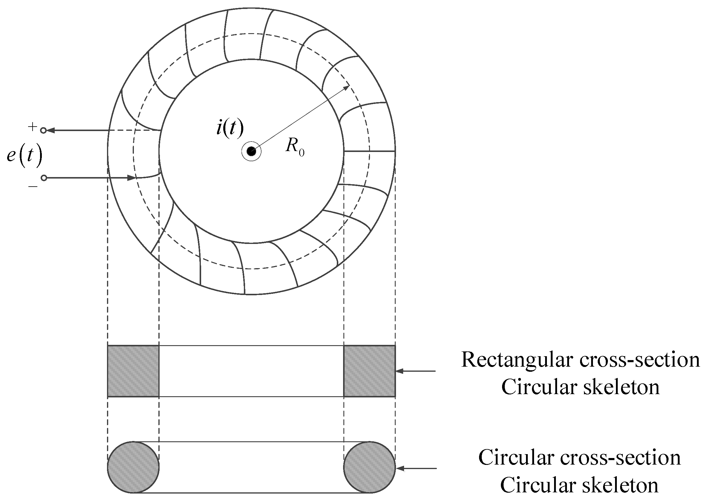
As shown in Figure 1, a Rogowski coil refers to a coil uniformly wound on a skeleton made of non-ferrous material. When a time-varying current i(t) flows along the central axis of the skeleton, a terminal voltage e(t) is induced, and i(t) can be recovered from e(t).
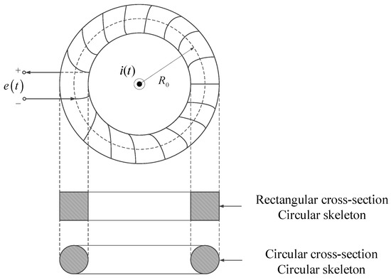
Figure 1.
The structure and measurement principle of Rogowski coils.
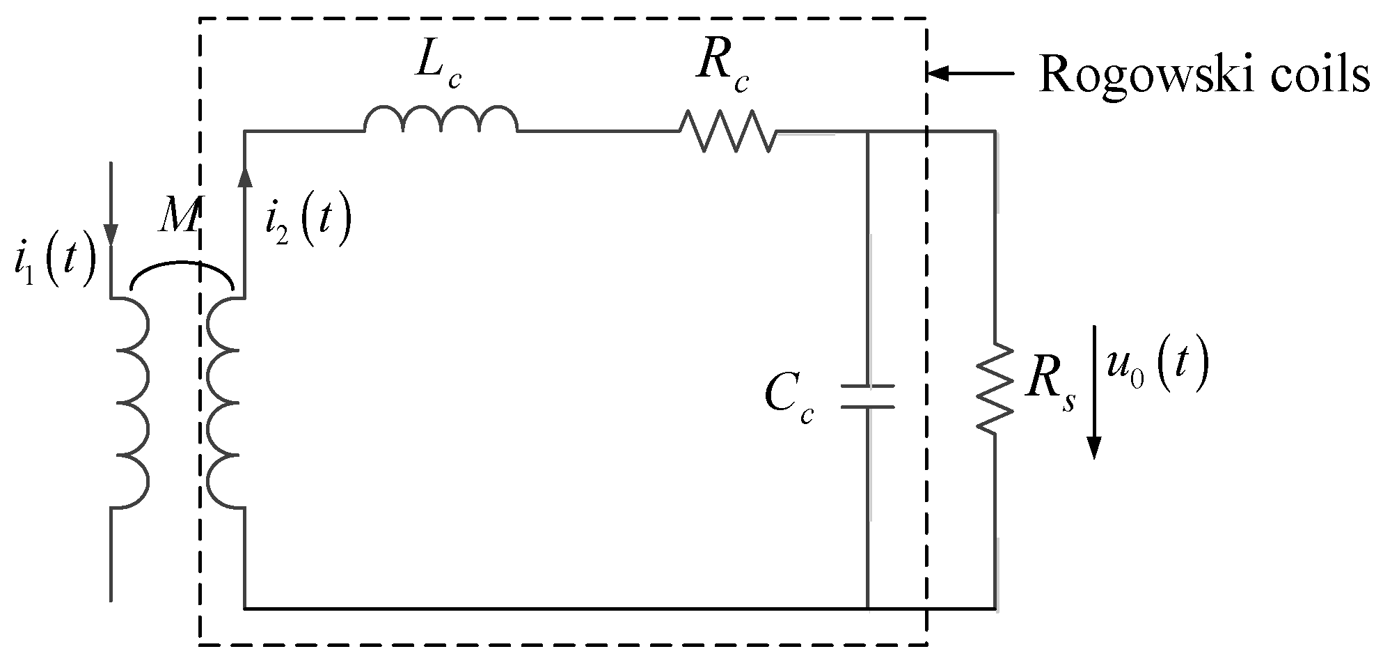
An equivalent circuit model of Rogowski coils is presented in Figure 2, where LC, RC, Cc, and RS are the self-inductance, internal resistance, stray capacitance, and external sampling resistance of the coil, respectively. M represents the mutual inductance of the coil and the current-carrying wire. The current to be measured and the current flowing through the coil are denoted by and , respectively [14].

Figure 2.
The equivalent circuit model of Rogowski coils.
In practical applications, it is necessary to integrate with integrator circuits to accurately extract the time profile of the measured current . According to different types of external signal processing circuits, the working states of Rogowski coils are usually divided into two self-integration and external integration [15,16].
Given sufficiently small or large , the voltage is approximately proportional to the measured current . Under this condition, Rogowski coils work under the self-integrating state, and a sampling resistor can be directly connected to complete a current measurement loop. It is straightforward to obtain the upper cut-off frequency and the lower cut-off frequency of the measurement circuit [8]
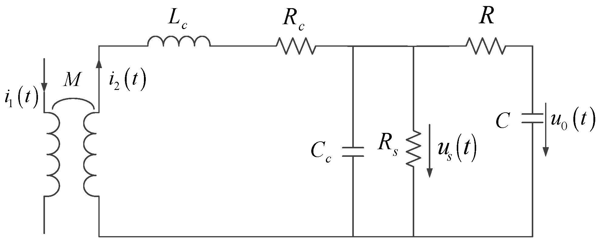
When the self-integrating condition is not satisfied, an RC integral circuit is added to the measurement circuit, as shown in Figure 3, where typically . The upper cut-off frequency and the lower cut-off frequency of the measurement circuit can be calculated as [17]

Figure 3.
The equivalent circuit diagram of external integral working state of Rogowski coil.
From Equations (1) and (2), it is seen that the bandwidth of Rogowski coils is determined by the internal resistance , sampling resistance , self-inductance or mutual inductance (, where N denotes the number of turns) and stray capacitance .
In general, the internal resistance and the mutual inductance have considerable influence on the low frequency characteristics of the measurement circuit yet little effect on the high frequency characteristics. Increasing brings little benefit of the amplitude-frequency gain, but it leads to worse low-frequency characteristics and narrower bandwidth. Therefore, should be reduced as much as possible. On the other hand, increased can improve the sensitivity and expand the bandwidth; hence, a larger M is usually favorable. As for the choice of the sampling resistance , there exists a tradeoff, since large leads to oscillation, while decrease of reduces the gain and signal-to-noise ratio.
The stray capacitance , which is the focus of this work, is one of the dominant factors affecting the high frequency response. From Equation (2), it is obvious that reducing the stray capacitance expands the bandwidth and improves the high frequency performance of Rogowski coils.
3. Stray Capacitance of Rogowski Coils
To extract the stray capacitance of Rogowski coils, we regard each turn of the winding as a single coil represented by lumped elements, and present a network model of the equivalent circuit of Rogowski coils in Figure 4, where and are the internal resistance and self-inductance of the i-th turn of the winding, respectively. represents the mutual inductance of the i-th turn and the current-carrying conductor, and denotes the mutual inductance of the i-th and k-th turns. Similarly, is the capacitance of the i-th turn and the shielding shell, while is the capacitance of the i-th and k-th turns of the winding.
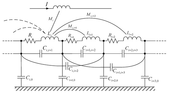
Figure 4.
A lumped network model of Rogowski coils.
3.1. A Network Model of the Stray Capacitance of Rogowski Coils
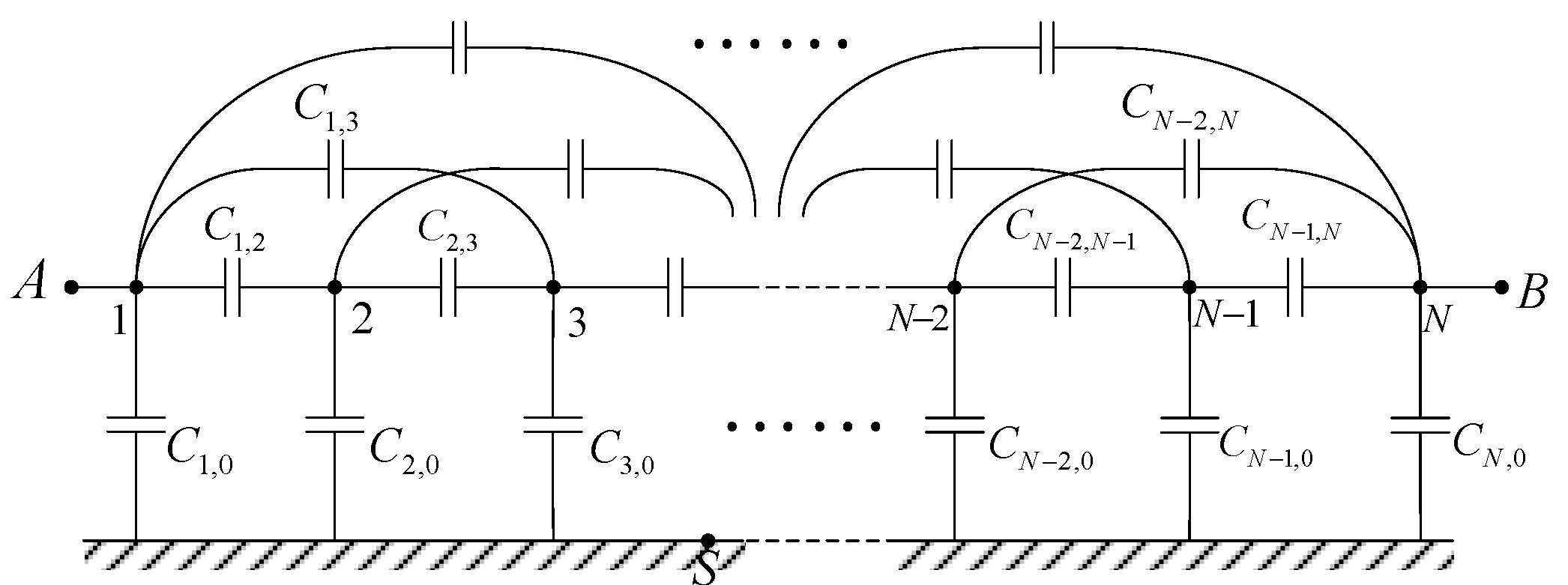
Based on Figure 4, the capacitance network of Rogowski coils is depicted in Figure 5, in which the edge effect of the winding at both ends is ignored [18]. In Figure 5, each marked node represents a single turn of the winding, and the grounding shield is modeled as a reference node S. The stray capacitance is defined as the lumped stray capacitance between the two terminal nodes A and B of Rogowski coils; thus, is referred to as hereinafter. After (N-2) times of the star-delta transformation, the intermediate nodes are eliminated step by step, and the π-type equivalent circuit of the stray capacitance network can be obtained, and the stray capacitance can be calculated accordingly. However, when the number of nodes is large, this approach is very cumbersome.
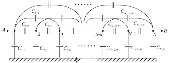
Figure 5.
A network model of the stray capacitance of Rogowski coils.
3.2. Simplified Model of the Stray Capacitance Network
Generally speaking, the stray capacitances among non-adjacent turns of the winding are much smaller than those of the adjacent turns [19]. In order to simplify the network, the capacitances among non-adjacent turns are excluded, and a simplified network model of the stray capacitance of Rogowski coils is obtained, which is shown in Figure 6, where is the inter-turn capacitance of adjacent turns of the winding, and the capacitance of each turn and the shielding is denoted by . It should be emphasized that since the two turns located at the two ends of the winding are also adjacent in space, the inter-turn capacitance between them cannot be ignored.
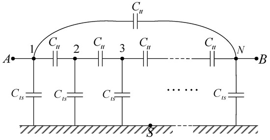
Figure 6.
Simplified model of the stray capacitance network of Rogowski coils.
By repeatedly implementing the star-delta transformation, can be easily calculated. Firstly, consider a network with only two nodes. The lumped stray capacitance is
When there are three nodes, we derive as
For models with more than three nodes, can be seen as a superposition of two components. The first component is the inter-turn capacitance between the two ends of the winding, namely . The second component is based on the simplified model in Figure 6, but of course is removed. The evaluation of can be achieved by adding one node to each end in turn. Note that , and , the following recursive formula can be obtained
Obviously, there is
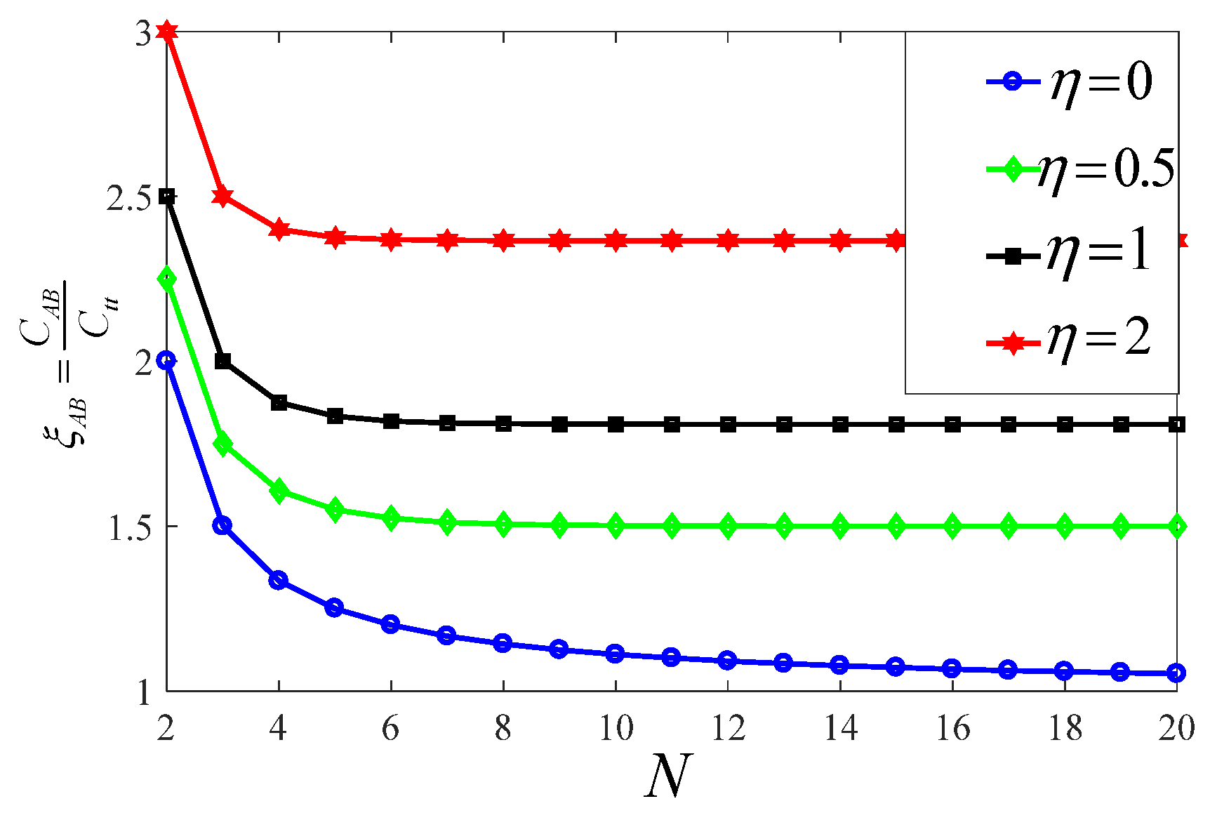
Let , then define
Figure 7 presents the variation of with the number of turns under various . It is observed that when N > 10, is very close to the limit . According to Equation (7),
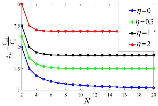
Figure 7.
Variation of coefficient value with number of turns.
In particular, if the shielding shell does not exist, the capacitance between the winding and the shell will not be included, i.e., the capacitance branches of all the junctions to the shielding shell in Figure 6 are disconnected; thus,
From the above analysis, as long as the values of and are known, the stray capacitance can be easily computed with Equation (8) or Equation (9). In addition, it is straightforward to conclude that reduction in either or would be beneficial to yield low . In the presence of a shielding case, the turn-to-turn capacitance can be computed by
where , is the length of a single turn of the winding, p is the distance between turns, h is the distance between turns and the shielding shell, is the radius of the winding conductor, and and are the thickness and relative permittivity of the wire insulation layer, respectively.
The approximate formula for the turn-to-shield capacitance is
where the definitions of all parameters are the same as those in Equation (10).
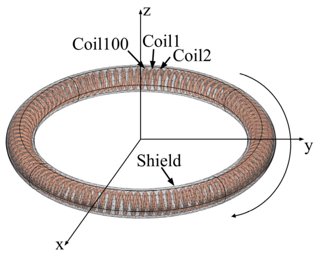
The simplified model of the stray capacitance as well as Equations (10) and (11) is validated by finite element (FEM) analysis using the commercial software COMSOL Multiphysics version 6.0. The geometry and mesh are depicted in Figure 8. The inner and outer radii of the skeleton are 56 mm and 64 mm, respectively. Both the coils and the shield are made of copper. The thickness of the grounded shield is 0.5 mm. The total number of turns is 100. It is worth noting that we intentionally disconnect adjacent turns of coils by including a small air gap, so that each turn can be regarded as an independent conductor. After exciting Coil1 with a static electric potential and setting other turns grounded, electrostatic simulation is carried out and total electric charge of each conductor can be calculated. Then by straightforward post processing, the stray capacitances of Coil1 and all other turns of the coils as well as the shield can be extracted. Due to the symmetry of the model, all mutual capacitances among the turns of coils capacitances can be obtained by exciting only Coil1.

Figure 8.
Geometry and mesh of the finite element model of Rogowski coils. (The reference values are mm, mm, mm).
The comparison of the proposed model against the FEM results is given in Table 1. Note that the FEM results in this table is grid-independent solutions, or in other words, we gradually increase the mesh density so that the values of are almost invariant. The resultant number pf tetrahedron elements are 638,331. It is seen that the results from the proposed method agree well with FEM solutions; thus, the accuracy of the simplified model of the stray capacitance as well as Equations (10) and (11) is justified. In addition, we must point out that substitution of the accurate Cts and Ctt from the FEM simulation into Equation (8) leads to a relative error of 0.7% in CAB. Therefore, the main error source in CAB is the approximation of Cts and Ctt by Equations (10) and (11), and our simplification of the capacitance network by ignoring coupling among non-adjacent turns of coils has very little influence on the accuracy.

Table 1.
Validation of the stray capacitance model.
3.3. Discussions of the Factors Affecting Stray Capacitance
In this subsection, the influencing factors of and is investigated, and measures to reduce the stray capacitance of Rogowski coils are put forward.
3.3.1. Investigations of Factors Affecting
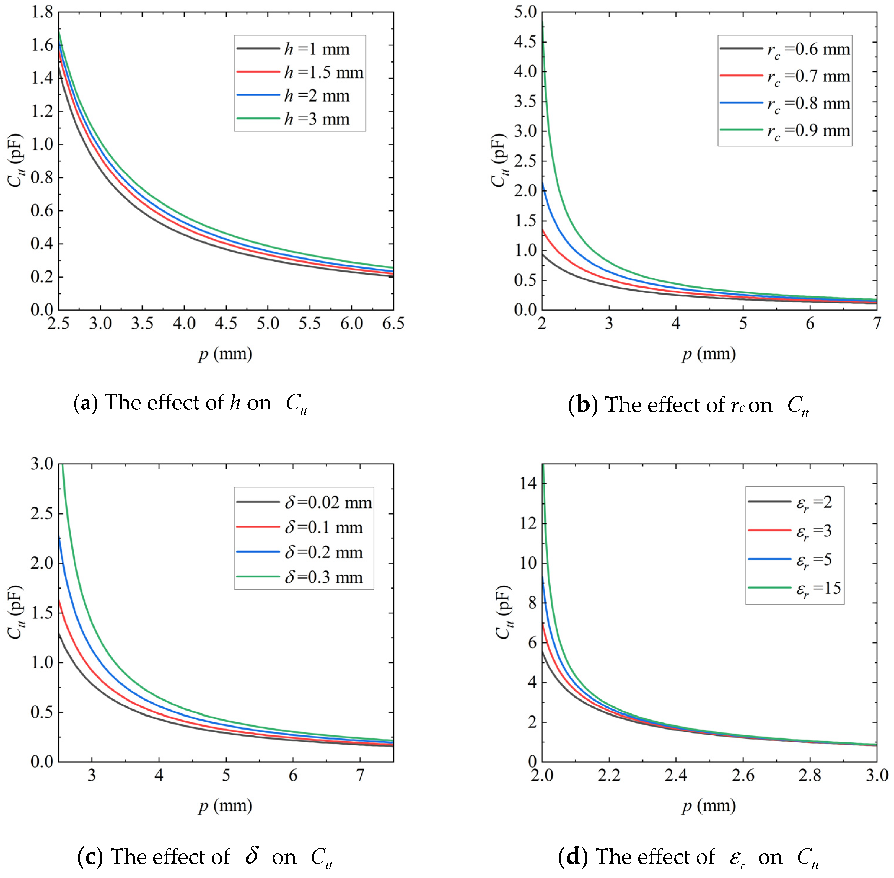
From Equation (10), it is obvious that is proportional to the length . The influences of h, rc, , and on Ctt are shown by Figure 9. It can be seen that under fixed , can be reduced by increasing the distance p among the adjacent turns, or decreasing h, , , and .
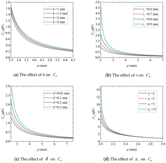
Figure 9.
Influence of each parameter on the value of the turn-to-turn capacitance . (The reference values are mm, mm, , mm, mm).
3.3.2. Investigations of Factors Affecting
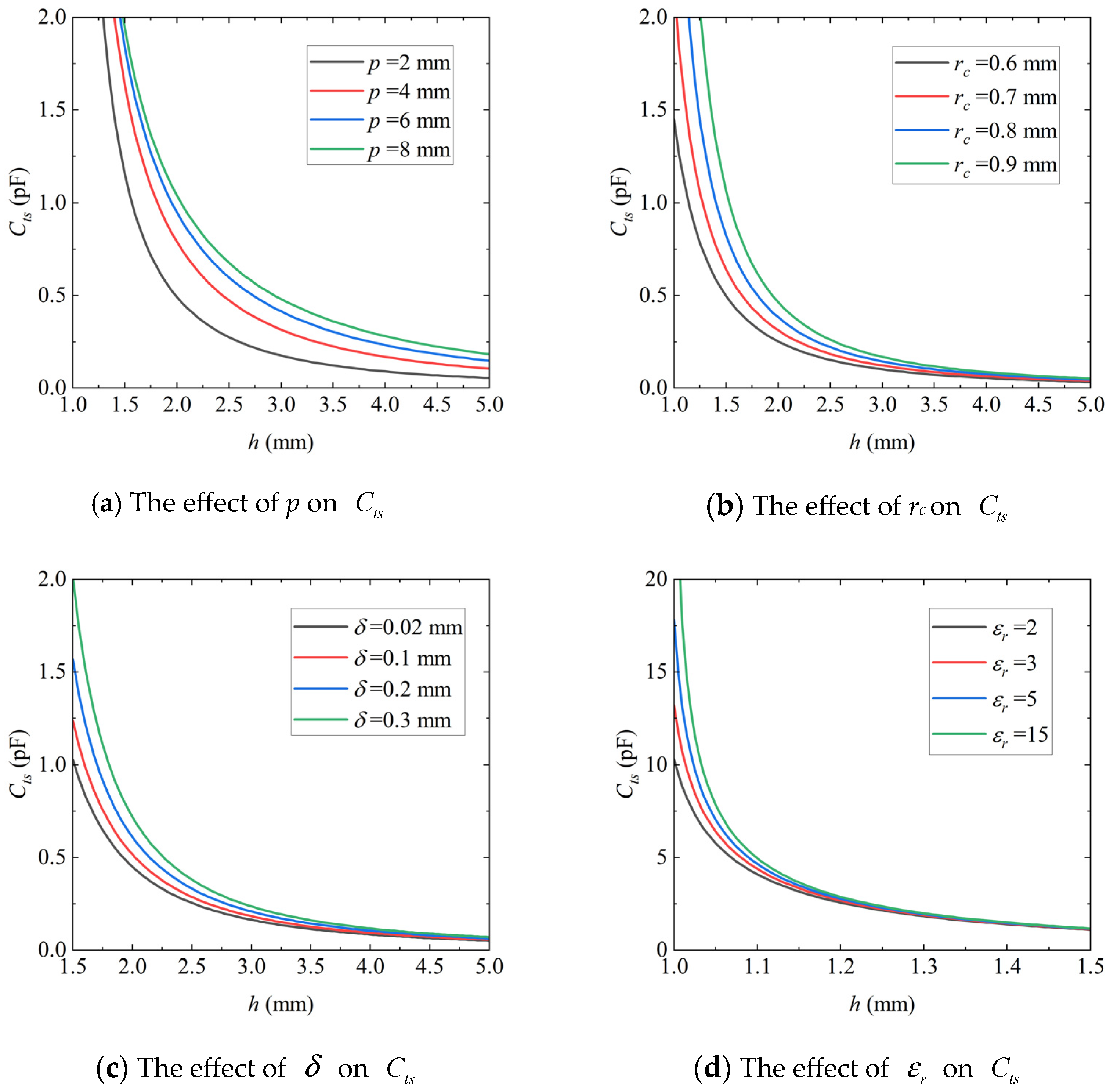
Similarly, is proportional to . The influences of h, rc, , and on Cts are given by Figure 10. It is seen that under constant , an increase of h and decrease of p, rc, , and result in reduced .
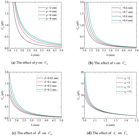
Figure 10.
Influence of each parameter on the capacitance between a single turn of the winding and the shielding shell . (The reference values are mm, mm, , mm, mm).
3.3.3. Measures to Reduce Stray Capacitance
Based on the above results, there exists a tradeoff regarding the selection of the turn-to-turn distance p and the distance h between the turns and shielding shell. Increasing p or decreasing h can reduce but increase . On the other hand, adjustment of p changes the number of turns N, which is directly related to the self-inductance and mutual inductance . As for h, this parameter is limited by space; thus, it cannot be chosen freely. Similarly, small winding conductor radius , wire insulation thickness , and are favorable for reduction of both capacitance and , but they are restricted in practical applications. For example, reducing leads to increased internal resistance and spoils the performance of Rogowski coils.
Last but not least, , , and are proportional to ; hence, shortening the length of the single-turn winding to simultaneously reduce these three parameters is favorable from the perspective of minimizing the stray capacitance. Since is approximately equal to the perimeter of the skeleton cross-section l, can be optimized by deliberate design of the cross-section of the skeleton of Rogowski coils so that is minimized.
It is worth emphasizing that the optimization must be implemented under the condition of invariant magnetic flux through the cross-section, or in other words, guaranteeing constant mutual inductance, so that the low-frequence performance of Rogowski coils is not affected.
4. Optimization of the Skeleton Cross-Section
In this section, the optimization of the shape of the cross-section of Rogowski coils is discussed. The goal is to minimize the perimeter of the cross-section under constant magnetic flux, so that the stray capacitance is reduced without compromising other performance indicators of Rogowski coils, e.g., the mutual inductance M.
4.1. Optimization of Skeletons of Three Common Shapes
4.1.1. Rectangular Cross-Section
A schematic of rectangular cross-section is depicted by Figure 11, in which a and b are the lengths of the edges of the cross-section, i is the measured current flowing through the center of the coil, and R1 is the inner radius of the skeleton. In the case of uniform winding, the magnetic flux through each turn of the winding is

Figure 11.
Skeleton with rectangular cross-section.
The optimization problem for the dimensions of a rectangular cross-section skeleton can be expressed as follows. Given fixed inner radius R1, measured current i, and perimeter l = 2(a + b), determine the relation between a and b, such that the magnetic flux through the rectangular cross-section is maximized.
In [20], a straightforward derivation is presented as follows. Substituting
into Equation (12) yields
The maximum is achieved when
namely
Recall Equation (13), when a and b satisfy
The rectangular cross-section is optimized.
4.1.2. Circular Cross-Section
The magnetic flux through the circular cross-section is
where d is the diameter of the circular cross-section.
If is fixed, the perimeter of the circular section is given by
The minimum perimeter l does not exist in this case. Although shortening the circumference makes the stray capacitance smaller, it also reduces the magnetic flux and thus the mutual inductance M. Therefore, a circular cross-section skeleton should be avoided from the perspective of keeping the mutual inductance unchanged while only minimizing the stray capacitance.
4.1.3. Oval Cross-Section
One of the anonymous reviewers reminded us of the fact that the adoption of rectangular cross-section imposes a sharp bending in the enameled-copper wire, inducing potential enamel rupture and wire shorting. Therefore, in practical applications, it is favorable to adopt shapes with rounded corners, referred to as oval cross-section. Figure 12 presents an example of oval cross-section, which consists of a rectangular domain and two half-circles. The magnetic flux through the oval cross-section is
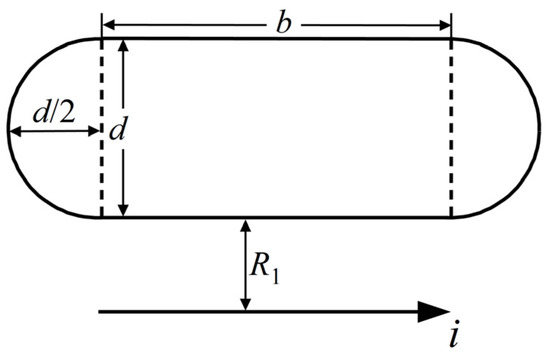
Figure 12.
Skeleton with oval cross-section, where d and b denote the radius of the half-circles and the length of the rectangular domain, respectively.
The perimeter of this cross-section is ; thus,
The magnetic flux can be recast as
Similar to the optimization of rectangular cross-section, the oval cross-section is optimized when , which results in a nonlinear equation (in terms of d) that can be efficiently solved by software such as MATLAB version 2022b and Mathematica version 12.0.
4.2. Optimal Design of the Skelenton Cross-Section
In this subsection, we consider an improved cross-section of the skeleton of Rogowski coils with smooth and convex boundary, as presented in Figure 13, where R1 and R3 are the inner and outer radii of the skeleton, respectively. Note that R1 is usually fixed to a pre-given value, there are four geometrical parameters remaining to be determined, namely z0, zmax, R2, and R3. The goal is to optimize these parameters to obtain a skeleton with the minimal perimeter under constant magnetic flux. To achieve this goal, a constrained variational problem is defined and solved.
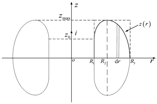
Figure 13.
Optimal skeleton cross-section for Rogowski coils.
4.2.1. The Constrained Variational Problem
As shown in Figure 13, the skeleton cross-section is in the z-r plane in the cylindrical coordinate system, and the center of the skeleton coincides with the coordinate origin O. The measured current i flows along the z axis. Assuming that the coil is wound uniformly and all turns are identical, their magnetic fluxes are equal due to symmetry. Now the remaining task is to find the skeleton cross-section with the shortest length of a single-turn winding under given magnetic flux.
To begin with, consider the magnitude of the magnetic flux density B at a point within skeleton cross-section
where is the magnetic permeability of the skeleton. Obviously, B is perpendicular to the z-r plane and independent of z; thus, the optimal cross-section should have an axis of symmetry perpendicular to the z-axis, which in our context is assumed to be the r-axis for convenience. As shown in Figure 11, only the upper half of the cross-section needs to be discussed, and the intersection points of its boundary and the r-axis are denoted by (R1, 0) and (R3, 0), respectively. Another point is that since the magnitude of B is proportional to 1/r, at least a portion of the boundary of the skeleton should lie on the straight-line r = R1 to yield as large magnetic flux as possible with unit perimeter. Assume that this portion is the line segment from (R1, 0) to (R1, z0). In the interval , the boundary z(r) should be a single-valued function. Based on the above discussions, obtaining the optimal skeleton cross-section can be attributed to the following tasks. In the interval , given the magnetic flux through the region surrounded by the curve z(r) and the straight line segment , find a curve z(r) with the shortest length.
When the inner radius R1 is large, the magnetic lines of force passing through the cross-section of the winding tend to be uniformly distributed, and the boundary of the optimal skeleton cross-section is close to a circle. As R1 decreases, this approximate circumference gradually compresses along the r-direction and partially coincides with the straight line r = R1, and extends along the z-axis, ensuring the shortest possible length of the cross-section circumference for a constant flux through the area it encloses. This indicates that there must exist a smooth and convex curve which is the contour of the optimal skeleton cross-section. The contour of the upper half of the optimal skeleton cross-section z(r) should have the following characteristics. Firstly, it should be composed of a straight line segment and a convex curve, and the straight line segment is tangential to the convex curve at the point of intersection. There should be, and there can only be, two such points on the convex curve, at which the first-order derivatives are infinite, and the two points should be the intersections of the convex curve with the straight lines and at the intersections and , i.e., and , respectively. In addition, the first-order derivative at a point on the convex curve is equal to zero, namely , and its corresponding z-coordinate is .
The magnetic flux through the area surrounded by the upper part of the curve and the segment is
With the definition , Equation (24) can be rewritten as
In the interval , the length of the upper half of the curve , which is denoted by , is calculated as
So far, the shortest perimeter problem has been attributed to the problem of determining the extreme value of the functional (26) under the constraints described by Equation (25). In summary, it can be formulated as the following conditional variational problem
4.2.2. Solution to the Constrained Variational Problem via Euler’s Method
A Lagrange multiplier is introduced to transform the original constrained variational problem into a free variational problem [21,22]. The resultant free variational problem is
Applying the Euler method to Equation (28) yields
Integrate Equation (29) to obtain
where C1 is a constant. Based on the previous discussion of the nature of the curve z(r), Equation (30) can be rewritten as
Integrating Equation (31) yields
where C2 and C3 are constants introduced during the integration. Obviously, from and , we conclude that and . Next, we sequentially determine C1, R2 satisfying , the Lagrange multiplier , zmax and z0.
Since z(R2) = zmax, the derivatives of z(r) satisfy , which can be substituted into Equation (31) to conclude , i.e., C1R1 = 1. Therefore, we have
Thus, Equation (32) can be recast as
When r = R1 and r = R3, the first-order derivatives of z(r) are and , respectively. Then, it is straightforward to see from Equation (31) that
The only possibility is
The combination of Equations (33) and (36) leads to
Substituting Equations (36) and (37) into Equation (35) gives
From Equation (34) and z(R3) = 0, it is deduced that
It is also obtained from Equation (34) and the continuity of z(r) at r = R2 that
Finally, by substituting Equations (33), (37), (38), (40), and (41) into Equation (34), the explicit formulation for z(r) of the optimal skeleton cross-section can be obtained as
where
and
4.3. Numerical Example
Equation (42) gives an explicit formulation for the perimeter of the optimal skeleton cross-section of Rogowski coils, yet the complex integral terms are not easy to compute in a pure analytical way. Therefore, the integral terms are calculated via some numerical approaches, e.g., Gaussian integration and trapezoidal rule.
Without losing generality, we assume cm and cm. Firstly, from Equations (30) and (31), cm and are obtained, respectively. Substitution of these two values into Equations (34) and (36) yields cm and cm.
Then, the right-hand side of Equation (42) is evaluated via Gaussian integration to obtain the optimal skeleton cross-section of Rogowski coils, which is plotted in Figure 14. It is worth noting that instead of Equation (42), an alternative solution approach to the constrained variational problem, i.e., Equation (27), is the finite element method (FEM), which is more general yet troublesome to implement. Detailed implementation of the FEM solution to Equation (27) is included in the Appendix A, and the results are also presented in Figure 14. It is observed that the results via Equation (42) agree well with those obtained by the FEM; thus, the correctness and accuracy of Equation (42) is justified.
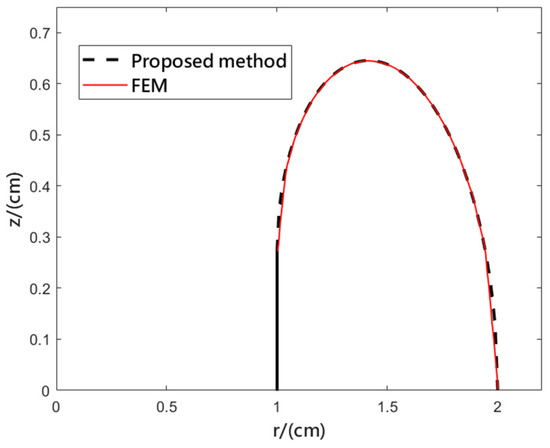
Figure 14.
Upper part (z > 0) of the optimal skeleton cross-section of Rogowski coils.
To further demonstrate the advantage of the optimized cross-section over the widely adopted rectangular, circular, and oval cross-sections, we present a brief performance comparison of the four shapes of cross-sections under identical = 1 cm and total magnetic flux in Table 2, where denotes the upper cut-off frequency normalized by the value corresponding to the rectangular cross-section under self-integration state, while corresponds to the external-integration state. It is worth noting that the geometry parameters of the rectangular and oval cross-sections have been optimized to make a fair comparison. The number of turns of the considered Rogowski coil is 70. The reference values of the parameters are mm, mm, , and mm.
Table 2.
Comparison of different shapes of skeleton cross-section.
First, it is observed that under fixed magnetic flux (namely identical LC) and = 1 cm, the rectangular skeleton requires the longest perimeter, and therefore exhibits the largest stray capacitance and the lowest upper cutoff frequencies. The proposed improvement of the cross-section of the skeleton results in the shortest perimeter and highest and , especially under the self-integration state. As for the external integration working state, the proposed cross-section leads to a cutoff frequency 6.4% higher than that of the rectangular cross-section.
Second, the performance of the oval cross-section is expected to be somewhere between those of the circular cross-section and rectangular cross-section, yet surprisingly this shape turns out to be the second-best choice. The stray capacitance and resistance are very close to those of the proposed optimized cross-section.
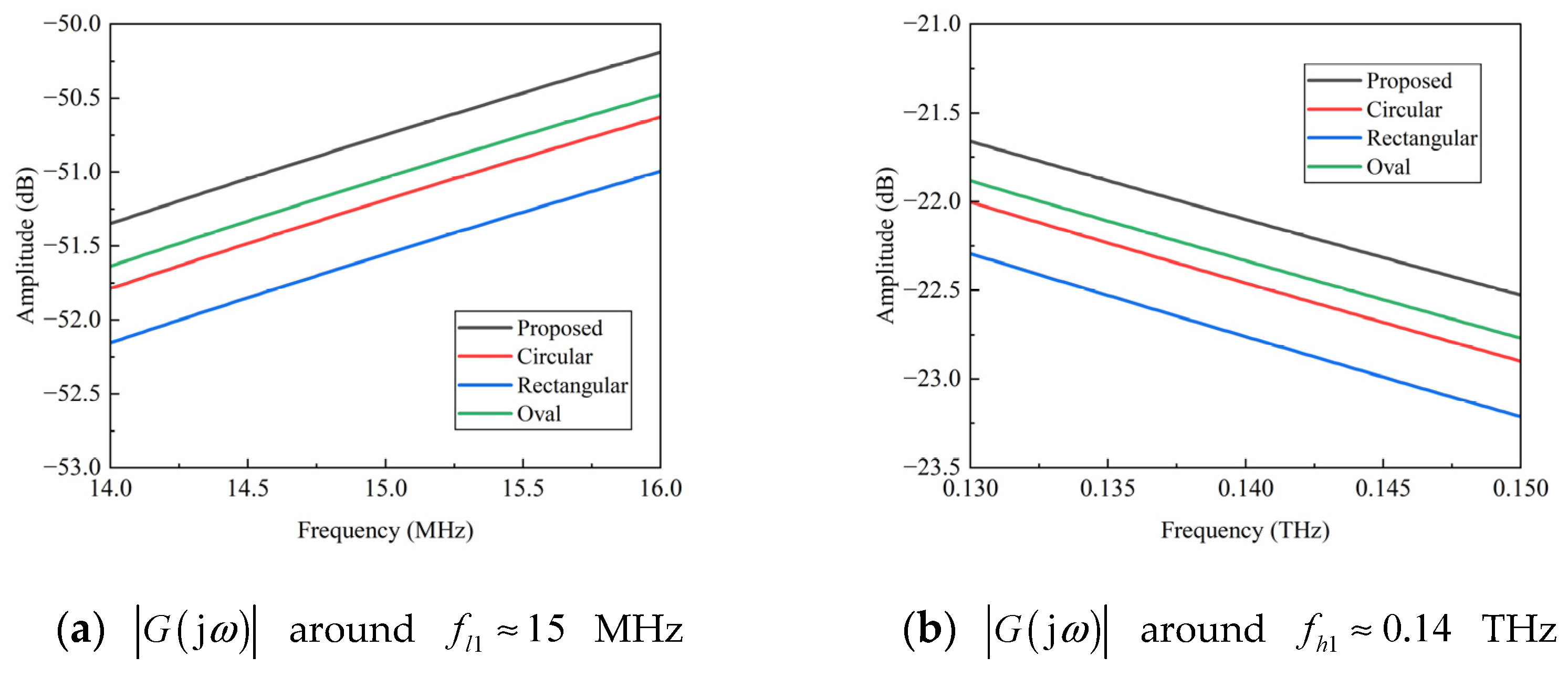
Third, the resistance Rc is also approximately proportional to the perimeter of the skeleton cross-section . Thus, the proposed method for minimization of l also leads to a reduction in Rc and the expansion of the bandwidth of the Rogowski coils under a self-integration state, because from Equation (1), it can be concluded that the lower cut-off frequency decreases under the reduced Rc. To justify this conclusion, we start with the transfer function of the self-integration coil in Figure 2
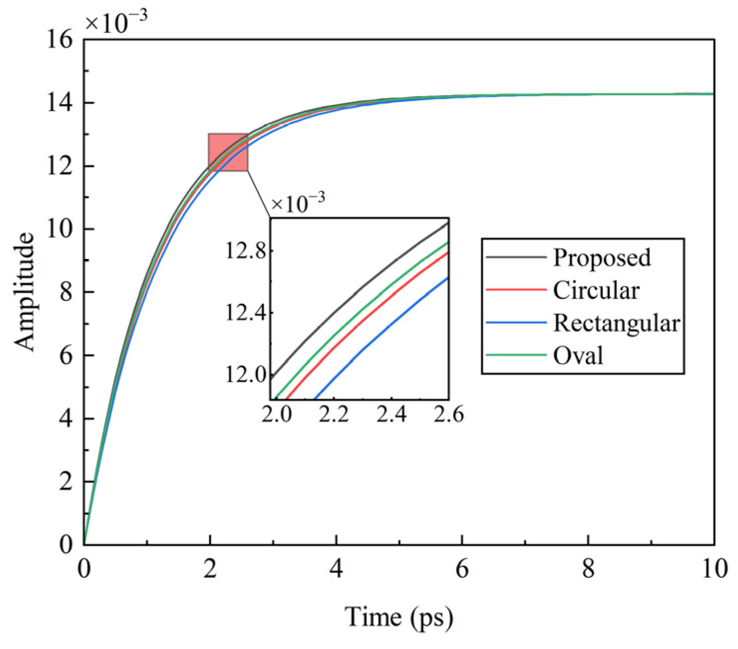
The frequency response around the lower cut-off frequency MHz and the uppercut-off frequency THz of the presented example are plotted in Figure 15a and Figure 15b, respectively. It is seen that in both low-frequency and high-frequency ranges, the proposed cross-section yields the highest transmission gain, while the rectangular cross-section exhibits the worst performance. To further evaluate the dynamic performance of the coils, Figure 16 depicts the step response of the self-integration coil. As expected, the proposed cross-section corresponds to the quickest response, indicating the largest overall bandwidth of this design. For comparison, the oval and circular cross-sections exhibit very close comparisons, while the rectangular cross-section leads to the longest rising time and thus the most unfavorable performance.
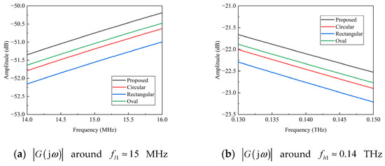
Figure 15.
Frequency response of Rogowski coils around lower and upper cutoff frequencies.
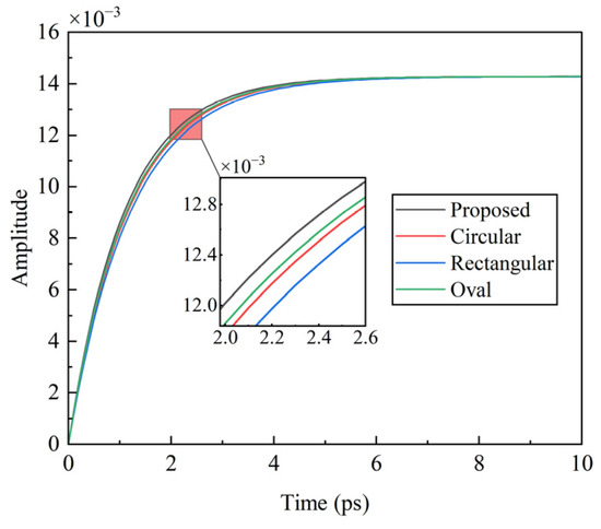
Figure 16.
Step responses of Rogowski coils with various cross-sections.
Last but not least, there are some extra benefits due to the reduction of the perimeter of the cross-section, including lighter weight and more compact structures.
5. Conclusions
The stray capacitance (=) is one of the main factors affecting the high frequency performance of Rogowski coils. Reducing the value of can expand the bandwidth and improve the high frequency performance of the coils.
The value of the lumped stray capacitance is approximately proportional to the length of a single-turn winding (which is approximately equal to the perimeter of the skeleton cross-section ); thus, the stray capacitance can be reduced via minimizing . Therefore, this manuscript is devoted to the optimization of the shape of the skeleton cross-section of Rogowski coils, so that l is minimized without affecting the total magnetic flux as well as the low frequency performance of the coils.
The stray capacitance of a Rogowski coils of rectangular cross-section skeleton is minimized when the length and the width satisfy , where is a pre-given inner radius of the skeleton. Similar optimization approach can be applied to the more realistic oval cross-section. On the other hand, the shortest perimeter that minimizes the stray capacitance under fixed magnetic flux does not exist for a circular cross-section skeleton.
Finally, under the condition that the total magnetic flux and the inductance of the coil are fixed, explicit formulations of the boundary of the optimal cross-section of the skeleton are deduced by solving a conditional variational problem. Numerical results demonstrate that the proposed optimization of the cross-section can effectively reduce the stray capacitance and resistance, leading to optimal bandwidth and dynamic response of Rogowski coils. The oval cross-section, as a combination of the rectangular and circular cross-sections, surprisingly outperforms the latter two options and exhibits very close performance to that of the proposed optimal cross-section.
Author Contributions
Conceptualization, J.W. and X.M.; Data curation, H.W.; Funding acquisition, J.W.; Methodology, J.W., H.W. and X.M.; Project administration, J.W.; Software, M.M.; Supervision, X.M.; Validation, J.W. and M.M.; Writing—original draft, J.W. and H.W. All authors have read and agreed to the published version of the manuscript.
Funding
This research was funded by National Key R&D Program of China under Grant 2021YFB2401700, and National Natural Science Foundation of China under grant 52207014.
Institutional Review Board Statement
Not applicable.
Informed Consent Statement
Not applicable.
Data Availability Statement
Data are available upon reasonable request to the corresponding author.
Conflicts of Interest
The authors declare no conflicts of interest.
Appendix A
This appendix presents the implementation details of the FEM solution to the constrained variational problem defined by Equation (20). Consider the interval , which is divided into n subintervals by n + 1 equidistant points . The length of the sub-intervals
By introducing the Lagrange multiplier and the definitions
the free variational problem to be minimized can be formulated as
Within each sub-interval, a linear interpolation of z(r)
is defined, where and are the function values of z(r) at and , respectively. Then the contribution of the i-th sub-interval to is
Substitution of Equation (A5) into Equation (A6) leads to
Accumulating all to obtain
To minimize , it is required that
Since z0 and zmax can be determined by the boundary conditions and are given by Equations (36) and (37), only n − 1 effective equations can be extracted. Substitution of Equation (A7) into Equation (A9) results in
where
The n − 1 nonlinear equations described by Equation (A10) are coupled to each other, yet numerical solutions via MATLAB or Mathematica is straightforward. The curve in the interval can be extracted in a similar manner.
In our context, MATLAB R2022b is adopted and the numbers of sampling point in both and are set to be 50. The FEM results in Figure 12 agree well with those from the analytical formulation. The slight difference may be induced by the approximation of the optimal curve by the linear interpolation defined by Equation (A5), and the unavoidable residual for solving coupled nonlinear equations.
References
- Abdi-Jalebi, E.; McMahon, R. High-Performance Low-Cost Rogowski Transducers and Accompanying Circuitry. IEEE Trans. Instrum. Meas. 2007, 56, 753–759. [Google Scholar] [CrossRef]
- Samimi, M.H.; Mahari, A.; Farahnakian, M.A.; Mohseni, H. The Rogowski Coil Principles and Applications: A Review. IEEE Sens. J. 2015, 15, 651–658. [Google Scholar] [CrossRef]
- Ramboz, J.D. Machinable Rogowski Coil, Design, and Calibration. Trans. Instrum. Meas. 1996, 45, 511–515. [Google Scholar] [CrossRef]
- Chen, Q.; Li, H.-b.; Huang, B.-x.; Dou, Q.-q. Rogowski Sensor for Plasma Current Measurement in J-TEXT. IEEE Sens. J. 2009, 9, 293–296. [Google Scholar]
- Liu, X.; Huang, H.; Jiao, C. Modeling and Analyzing the Mutual Inductance of Rogowski Coils of Arbitrary Skeleton. Sensors 2019, 19, 3397. [Google Scholar] [CrossRef] [PubMed]
- Ferkovic, L.; Ilic, D.; Lenicek, I. Influence of Axial Inclination of the Primary Conductor on Mutual Inductance of a Precise Rogowski Coil. IEEE Trans. Instrum. Meas. 2015, 64, 3045–3054. [Google Scholar] [CrossRef]
- Tao, T.; Zhao, Z.; Ma, W.; Pan, Q.; Hu, A. Design of PCB Rogowski Coil and Analysis of Anti-interference Property. IEEE Trans. Electromagn. Compat. 2016, 58, 344–355. [Google Scholar] [CrossRef]
- Jie, B. High Current Measurement; China Machine Press: Beijing, China, 1987; pp. 181–198. (In Chinese) [Google Scholar]
- Chiampi, M.; Crotti, G.; Morando, A. Evaluation of Flexible Rogowski Coil Performances in Power Frequency Applications. IEEE Trans. Instrum. Meas. 2011, 60, 854–862. [Google Scholar] [CrossRef]
- Li, W. Theoretical Research and Practice of Large Current Measurement Sensing Based on Rogowski Coil. Ph.D. Thesis, Huazhong University of Science and Technology, Wuhan, China, 2005. (In Chinese). [Google Scholar]
- Mingotti, A.; Costa, F.; Peretto, L.; Tinarelli, R.; Mazza, P. Modeling Stray Capacitances of High-Voltage Capacitive Dividers for Conventional Measurement Setups. Energies 2021, 14, 1262. [Google Scholar] [CrossRef]
- Yue, X.; Zhu, G.; Wang, J.V.; Deng, X.; Wang, Q. PCB Rogowski Coils for Capacitors Current Measurement in System Stability Enhancement. Electronics 2023, 12, 1099. [Google Scholar] [CrossRef]
- Robles, G.; Shafiq, M.; Martínez-Tarifa, J.M. Designing a Rogowski Coil with Particle Swarm Optimization. Proceedings 2019, 4, 10. [Google Scholar]
- Zhao, T. Optimized Design of Rogowski Coil for Pulse Current Measurement. Master’s Thesis, Huazhong University of Science and Technology, Wuhan, China, 2005. (In Chinese). [Google Scholar]
- Metwally, I.A. Self-Integrating Rogowski Coil for High-Impulse Current Measurement. IEEE Trans. Instrum. Meas. 2010, 59, 353–360. [Google Scholar] [CrossRef]
- Zhang, R.; Chen, C.; Wang, C. High Voltage Test Technology; Tsinghua University Press: Beijing, China, 2009. (In Chinese) [Google Scholar]
- Jiao, C.; Zhang, J.; Zhao, Z.; Zhang, Z.; Fan, Y. Research on Small Square PCB Rogowski Coil Measuring Transient Current in the Power Electronics Devices. Sensors 2019, 19, 4176. [Google Scholar] [CrossRef]
- Dalessandro, L.; Cavalcante, F.S.; Kolar, J.W. Self-Capacitance of High-Voltage Transformers. IEEE Trans. Power Electron. 2007, 22, 2081–2092. [Google Scholar] [CrossRef]
- Qin, Y.; Holmes, T.W. A Study on Stray Capacitance Modeling of Inductors by Using the Finite Element Method. IEEE Trans. Electromagn. Compat. 2001, 43, 88–93. [Google Scholar] [CrossRef]
- Atabekov, G.I. Several Problems of Theoretical Electro-Engineering; National Defence Industry Press: Beijing, China, 1958. (In Chinese) [Google Scholar]
- Liang, L. Variational Principles and Their Applications in Mechanics and Electromagnetism; Harbin Engineering University Press: Harbin, China, 2011; ISBN 978-7-5661-0044-3. (In Chinese) [Google Scholar]
- Reddy, J.N. Energy Principles and Variational Methods in Applied Mechanics; John Wiley & Sons: Hoboken, NJ, USA, 2017. [Google Scholar]


Disclaimer/Publisher’s Note: The statements, opinions and data contained in all publications are solely those of the individual author(s) and contributor(s) and not of MDPI and/or the editor(s). MDPI and/or the editor(s) disclaim responsibility for any injury to people or property resulting from any ideas, methods, instructions or products referred to in the content. |
© 2024 by the authors. Licensee MDPI, Basel, Switzerland. This article is an open access article distributed under the terms and conditions of the Creative Commons Attribution (CC BY) license (https://creativecommons.org/licenses/by/4.0/).