Abstract
The efficient operation and intelligent upgrading of public transportation can effectively enhance the attractiveness of conventional public transportation. In order to improve the delicacy management level of bus operations, this study designed a new dynamic optimization model for single-line bus operations with the dual optimization objectives of the lowest passenger travel cost and lowest operation cost, using a combination of the strategy of stop-skipping control and local route optimization. Simulated annealing (SA) was introduced into the genetic algorithm (GA) to design a hybrid heuristic algorithm for model solving. The effectiveness of the optimization model and the hybrid algorithm were verified and evaluated by using the No. 115 bus line in Ganzhou City as an example. The results showed that the proposed optimization model had a good usability, which can effectively improve the average vehicle speed, shorten the overall waiting time of passengers, and enhance the operational efficiency of the line. The hybrid algorithm saw significant improvement in terms of the iteration speed and the quality of the optimal solution compared with the conventional genetic algorithm.
1. Introduction
The priority development of public transportation as an important way to alleviate urban traffic congestion has long been a consensus, however, with the continuous development of the transportation industry, the complexity of the urban road traffic operating environment is not what it used to be, so traditional macro-regulation methods have not been able to solve the existing urban road space–time resource supply and demand contradiction. The current methods for public transportation scheduling can be divided into static scheduling and dynamic scheduling. Static scheduling refers to the layout planning and scheduling program of bus routes based on the historical passenger flows of routes, the capacity resources of bus-operating companies, etc., and its execution time is usually annual, quarterly, monthly, etc. [1]. Vehicle departure intervals, via paths and stops, strictly adhere to a pre-established plan and do not consider temporary passenger flow changes or road traffic information changes [2]. Dynamic scheduling is the adjustment of static scheduling during actual operation. It uses a new generation of information technologies, such as vehicle networking and big data, to obtain the real-time situation of passenger flow, road network conditions, and control information and make targeted adjustments to the pre-established scheduling plan. Dynamic scheduling is an important supplement to the traditional static scheduling methods, and when used properly, can effectively improve the level of bus intelligence and service level, so that passengers enjoy a more convenient bus travel experience. Common dynamic scheduling methods include the intelligent optimization of departure time, real-time operation control, and multi-mode combined operation, etc. [3]. Among them, the real-time operation control strategy is an important method for improving the efficiency of vehicle operations and turnover efficiency, which can be divided into the two categories of inter-station control and station control according to the different scope of the influence of the method of implementation.
Inter-station control strategies refer to the regulation of the driving process of buses in the zones between stations [4], including interval speed induction, signal priority, etc. Daganzo and Pilachowski analyzed the mode of action and the improvement effect of traditional control methods on the phenomenon of bus crosstown, and proposed a control scheme that can adaptively improve the cruising speed of this vehicle according to its front and rear speeds, which can automatically compensate for the driver’s driving behavior and the effects of traffic delays on the route and has low data requirements [5]. Teng and Jin proposed a bus speed induction method based on a dynamic headway deviation threshold by analyzing vehicle GPS data, which can suppress the increasing trend of headway deviation and improve the reliability of line operations [6]. They proposed a control strategy with two-layer control coefficients, which takes the nonlinear characteristics of the boarding process into consideration and establishes a combined regulation scheme for speed induction in the bus zoning section [7]. Estrada et al. theoretically calculated the high and low impacts of individual disturbances and changes in operating status on the stability of the whole bus line, determining the optimal speed control in signalized sections after comparing the optimization effects of multiple strategies [8]. Yang et al. proposed a BRT-applicable rapid pre-detection signal prioritization strategy in order to address the shortcomings of the traditional transit signal priority, and the four simulation scenarios from their experimental results showed that the pre-detection signal prioritization approach with intersection coordination had the best utility, reducing 67.4% of intersection delays and more than 40% of transit delays, with the intersection congestion time for private vehicles being similarly reduced [9]. Similar to the idea of Coordinated Transit Priority proposed by Ma et al. [10], Anderson et al. proposed the concept of Conditional Signal Priority (CSP) and optimized it using a Brownian-Motion-based mathematical model, which not only improves the reliability of transit, but also reduces the number of priority requests by more than 50% compared to normal signal priority [11].
Inter-station control has excellent results, which can effectively improve the stability of line vehicles, enhance the uniformity of headway spacing, and improve traditional bus crosstown and delay problems. However, the realization of this type of control method is highly dependent on the vehicle–road–dispatch center, real-time communication technology, and automatic driving technology. Although the current research has achieved rich results, there is still a certain distance to its practical application. In addition, some scholars believe that its safety also needs more research and verification [12].
Station control strategies are used in the process of controlling vehicles at certain stations on a route, including both the bus-holding strategy and stop-skipping strategy. The bus-holding strategy refers to the control of a bus to increase its dwell time at a stop in order to maintain distance from the vehicle in front of it or for other reasons [13]. The stop-skipping strategy refers to the control of a bus that skips directly over a stop without stopping [14]. Delgado et al. developed a plan update model for transit corridor operations using a vehicle that includes a limit on the number of boarding passengers with a hold-up strategy, reducing the total operating costs by more than 22% compared to a blank group [15,16]. Building on this framework, the team further proposed an HBLRT control method that considers a more balanced vehicle load factor [17]. Compared with the preceding studies, this method can reduce the expected waiting time by 6.3% and provide passengers with better ride comfort, with the computation time also being shortened. Xuan et al. proposed a series of vehicle arrival delay difference dynamic control strategies based on virtual schedules to address the problem of the general station-keeping strategy that schedule slack tends to cause vehicle speed reduction, which greatly reduces the delay rate of the vehicle. Their method can reduce the slack time by 40% more than the conventional schedule-based method [18]. Bartholdi and Eisenstein also abandoned the concept of a bus schedule and carried out the automatic equalization of line vehicles through two control parameters, which can still maintain its improvement effect in the face of large traffic disturbances. The method was successfully verified on a bus line in Atlanta [19]. Zheng studied the application prospect and realization path of vehicle–vehicle communication technology in the field of public transportation and established a vehicle over-stop scheduling model with multiple objectives such as passenger waiting time, additional waiting time, stopping time, and bus operation cost, ultimately proving that the model can reduce passenger travel delays and company operation costs through simulation on a bus line in Beijing [20]. In order to reduce the impact of station-crossing on passengers’ future trips, Gkiotsalitis developed a rolling horizon station-crossing model and a policy generation mechanism, which can solve a small-scale scheduling problems to the global optimum [21]. Chen et al. proposed a real-time bus combination control method based on station-keeping fuzzy controllers, which optimizes the parameters of the affiliation function through the genetic principle, effectively improves the headway of the line, and reduces the waiting time of passengers [22]. There are also some studies that have made some contributions to the innovation of solving mature models, and so on [23,24,25,26]. The station control method is relatively easy to realize, and can quickly restore the normal operation of a line to improve the efficiency of vehicle operation. However, when carrying out station control, it is necessary to carefully and comprehensively consider the conditions for the implementation of the control to avoid causing excessive negative impacts and psychological discomfort on passengers.
Conventional buses need to run with fixed bus stops and a driving path, and this path is generally not due to passenger flow, time, weather, and other external factors and changes. However, the implementation of local and limited dynamic adjustment and the restoration of buses’ running paths according to the actual situation of bus operation can also improve the operational efficiency of buses, which has been verified in the operational scenarios of demand-responsive buses. Although there are obvious differences between demand-responsive buses and conventional buses, it is undoubtedly theoretically feasible to optimize conventional routes with local and limited dynamic adjustments by referring to the idea of demand-responsive bus route generation and optimization.
For the evaluation of the operating conditions and optimization recommendations for conventional bus routes, Foletta et al. provided a solution for the design of bus networks in commercial urban areas, which is able to provide a regional perspective on route regeneration and route service frequency adjustment recommendations while evaluating the levels of existing routes, where the number of buses and amount of growth in passenger demand are the key influencing factors on network regeneration [27]. The equilibrium process and computational framework between service-level-related and cost-related influences in a transit system were analyzed from the VRP problem, and a dual-objective model for solving the transit problem was also provided by Joaquín et al. [28] Fan and Machemehl added the concept of “spatial equity” to the process of transit network evaluation and redesign, and found a balance between the number of passenger transfers and the operational benefits through the PTNRP-AEI bi-level optimization model [29]. Similar concepts were also mentioned in the study of Muhammad et al. [30], which mainly examined the rationality of urban bus stops and network settings from the perspective of passengers and designed an efficient genetic algorithm to obtain a high-quality solution. Wang et al. carried out an in-depth excavation of passengers’ OD information with archived ADCS data in Beijing and inferred the travel chain based on the characteristics of the individual travel patterns and the geographic proximity of the bus lines. Their results can be used to infer travel chains based on the individual travel pattern characteristics and the geographic proximity relationships between bus lines, and also provide reference suggestions for the evaluation of bus routes [31]. In addition, other influencing factors and assessment methods, including service gravity level [32], path demand potential [33], passenger travel time window constraints [34], and heterogeneous travel demand [35], have also received attention and research from scholars. Research on route generation and path optimization for bus routes is a hot issue in this field. Lin and Wong defined and investigated a multi-objective programming approach for feeder bus route determination, where the input values of the model do not need to be exact, but can be replaced by a fuzzy range, which facilitates the planners of customized bus routes to formulate operations and alternatives in an efficient and systematic way [36]. Lyu et al. proposed a model called CB -Planner, a customized bus-route-planning framework and heuristic solution that co-optimizes ride locations, route alignments, departure moments, and passenger choice probabilities, saving significant operational costs by moderately increasing travel time [37]. Huang et al. developed a hierarchical two-stage dynamic and static customized bus network service optimization model based on the fundamentals of the branch-and-bound method, and developed an approximate accurate solution algorithm to optimize the passenger service level of the original customized bus routes [38]. Ma et al. used the Bertsimas–Sim robust optimization theory to transform a model containing unknown parameters to solve a customized bus route planning problem containing multiple yards and stations, saving 42.11% of computation time compared with the general genetic algorithm [39]. Shen et al. decomposed the customized bus route design into a vehicle route problem with a time window and a passenger–vehicle bilateral matching problem, designing an H-R bilateral matching algorithm to solve the problem that achieved a passenger service rate of 88.5% in a real example in Tianjin [40]. The method also had a good performance in the problem scenario of Dunbar et al. [41]. Qiu established a three-layer logit model of passenger travel mode choice for the product characteristics and operation modes of customized buses, used the improved DBSCAN algorithm to complete the demand clustering, and finally established a path optimization model for customized buses that includes random user equilibrium and a time window [42].
In summary, scholars have achieved rich results in the field of bus operation optimization and formed a relatively perfect theoretical system. However, the existing research still has room for further optimization in the following aspects:
- (1)
- Some scholars simply used one of the strategies of bus-holding, stop-skipping, or signal control to avoid bus crosstown or late buses, which is for the control of two adjacent buses, without considering that changes in the status of adjacent buses will have an impact on the overall operation of the bus line, so the final scheduling program has a large optimization space.
- (2)
- Research on the real-time dynamic adjustment of bus running routes is limited to demand-responsive buses, and has not been applied to the operation optimization of conventional buses. There is a lack of research on the possible impacts of the localized and limited dynamic adjustment optimization of conventional bus running routes, which is not conducive to releasing the full potential of the bus system or improving the refinement level of bus operations.
Based on the existing research, this study aims to comprehensively quantify and analyze the operation process based on urban traffic multi-source data for single-line buses, determine feasible vehicle operation control strategies, and establish a dynamic synergistic optimization model based on a combined strategy to optimize and improve bus operation and intelligent regulation and explore feasible evolutionary algorithms and solution schemes. The main research contents of this paper are as follows:
- (1)
- From the perspective of overall system optimization, a dynamic control strategy for public transportation is proposed by combining bus-skipping control and operation path optimization.
- (2)
- With the dual optimization objectives of minimizing bus operation costs and minimizing passenger travel costs, the optimization objectives and constraints are clarified and a dynamic optimization model for single-line bus operations is established.
- (3)
- A hybrid heuristic algorithm based on simulated annealing principles and the genetic algorithm is designed for the model characteristics, based on which, a two-stage optimization model-solving scheme is proposed.
2. Dynamic Optimization Strategies for Public Transportation Operations
2.1. Research Scenario Definition
The research scenario is a unidirectional bus line with several bus stops. During the operating time of the line, each bus runs unidirectionally from the first stop to the last stop, and it is not allowed to make a U-turn or overtake the vehicle in front of it during the traveling process. The implementation process of the dynamic optimal scheduling method of bus operation can be described as follows: firstly, the passenger flow during the whole day is obtained according to historical data or model prediction, and this information and traffic data such as the road conditions and the initial scheduling scheme are input into the dynamic optimization model of vehicle operation to generate the initial station pool; subsequently, the judgment and generation of the scheduling station pool and feasible paths are carried out. Finally, the optimal operation scheme for public transportation is output.
2.2. Stop-Skipping Strategy
Skipping a stop means that passengers disembarking at the stop must spend more time waiting for the next bus or choose to disembark at a nearby stop, making the passengers’ traveling experience decline. Therefore, the use of the stop-skipping strategy must fully consider the actual level of passenger demand and the distribution characteristics of the line. To improve the overall operational efficiency of the line, a reasonable start threshold should be set as far as possible to reduce the negative impact of bus skipping on the passenger experience.
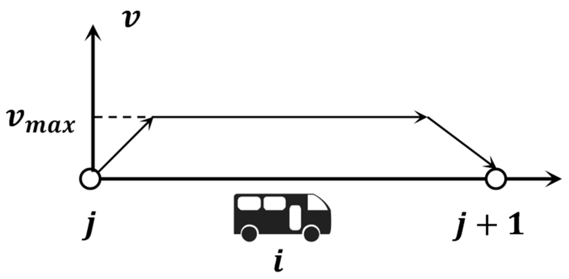
Suppose that, at some point in time, a bus on the route is about to arrive at bus stop , where the adjacent previous bus stop is and the next stop is . Taking the interval between stop and as an example, as shown in Figure 1, the bus operation process can be described as follows: at the very first moment, bus starts traveling with uniform acceleration from stop , and the speed reaches the highest speed of the interval operation and is then maintained; when near stop , bus enters into the process of uniform deceleration until its speed is reduced to 0, and stays at stop .

Figure 1.
Bus travel speed change process between stops.
Figure 2 shows the process of a bus traveling continuously between two or more bus stops. Point is the location where bus has the greatest speed and is about to enter the deceleration process as it travels from stop to . Similarly, point is the location where bus has just completed the acceleration process, and speed is reached.
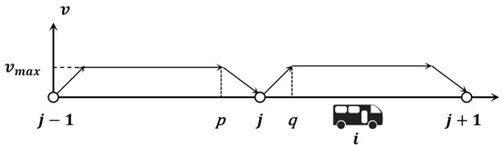
Figure 2.
Bus travel speed change process for continuous travel.
When the stop-skipping strategy is not adopted, the operation process between and can be divided into three phases: deceleration to stop, passengers embarking or disembarking, and accelerating to normal speed. The total running time consists of deceleration time , embark/disembark time , and acceleration time : . The additional cost of bus operations can be described as , where is the control variable of the bus deceleration and acceleration costs and is the control variable for the cost of the bus-stopping operation time at stop .
When adopting the stop-skipping strategy, i.e., bus travels from point at a constant speed until it passes point , the total running time . The additional cost of bus operations and the cost of the stopping time at stop is 0. However, stop-skipping will lead to passengers waiting at stop not being able to get on the bus and passengers on bus not being able to disembark at stop , so it is considered that there needs to be stop-skipping penalty cost, which can be described as , where and are the control variables of passenger loss costs and and are the numbers of passengers needing to embark/disembark.
In summary, the combined bus stop-skipping strategy in this study can be described as follows:
In the above equation, and are the thresholds for the activation of embarking and disembarking for stop-skipping control. When the number of passengers waiting to ride the bus or the number of passengers disembarking the bus exceeds this threshold, the over-stop control is invalid, otherwise, the cost calculation and a comparison of different strategies will be carried out to select the best strategy.
2.3. Path Optimization Strategy
In order to ensure driving safety and improve operational efficiency, conventional public transportation vehicles have a fixed path and station. However, in the case of the local stop-skipping control of bus routes, a reasonable limited path adjustment and optimization strategy can be taken in order to avoid road congestion or other reasons for operational delays. When it is feasible to adopt the stop-skipping strategy at stop and real-time traffic information shows that short-term congestion will occur nearby stop , the path optimization strategy can be judged and implemented.
The path optimization strategy can be carried out in two steps:
- (1)
- Vehicle operation topology network construction with branching.
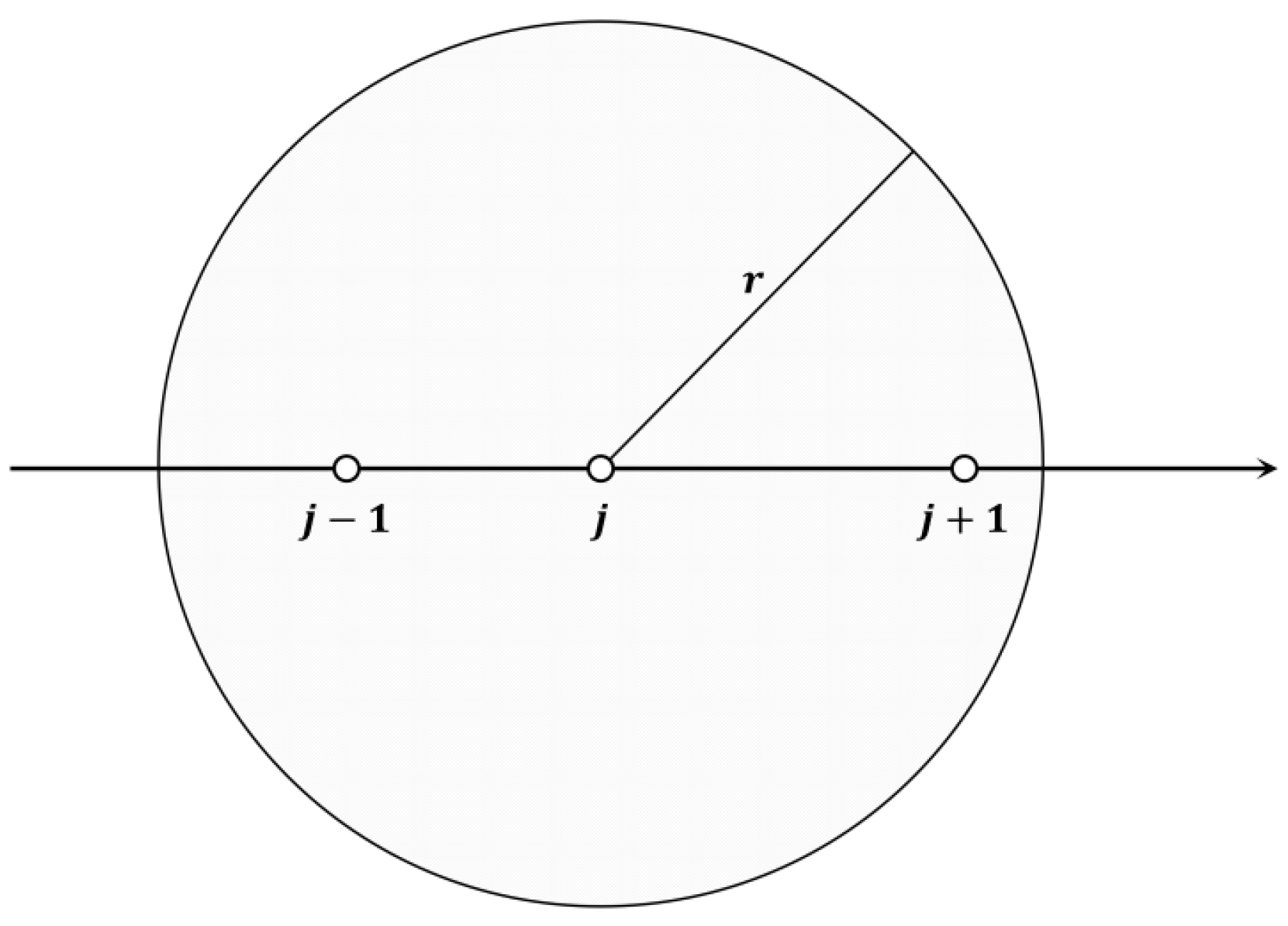
The basic domain for feasible path selection is constructed first. In order to reduce the number of searches for invalid nodes during path generation, the basic feasible domain of nodes is delineated, as shown in Figure 3. The search domain has as its center and as its radius. As the bus does not experience the deceleration, stopping, and acceleration process when traveling over the stop, the average speed of the interval will be higher than that of regular driving, so the range diffusion control coefficient is set to appropriately expand the search range and avoid the truncation of available paths due to the loss of some nodes. In this paper, we take .

Figure 3.
Path feasible domain search range.
Next, network weight filling and path generation are performed. The scenario targeted in this study is variable path planning under a future travel state, which faces many uncertainties and large dynamic changes in traffic flow. The Co-evolutionary Path Optimization (CEPO) method can deal with multi-source traffic information more efficiently and reflect the evolution trend of the traffic environment of the road section in the future period better, so this method is adopted for the planning of dynamic paths.
Considering the main influencing factors in the operation scenario of public transportation, this study selects the average roadway speed and average node delay as the key indicators of roadway network traffic parameters . There are:
In the above equation, denotes the average delay incurred by the bus while passing through the node from to ; denotes the average speed of the bus; is the error between the predicted and actual values of the roadway network traffic parameters at the moment; and is a time-varying function that describes the relationship between the roadway network traffic parameters over time.
- (2)
- Bus operation strategy construction based on relaxation time window.
The construction of the path optimization strategy is carried out with reference to the implementation of the vehicle crossing station combination control strategy. Supposing that, at a certain point in time, bus is about to arrive at stop and will execute the stop-skipping control strategy, the intended traveling path of bus along the stop →stop →stop is , and the feasible optimization paths are ,, …….. The movement process of bus can be approximated to divide it into two components: traveling on the roadway and passing through the stop.
Taking path as an example, the total length of the path is specified as , the average traveling speed is , the total number of buses passing through the stops is , and the average waiting time at the stops is . It is easy to determine that the traveling time through the path is . The cost can be characterized as , where and are the control parameters corresponding to the average section speed and average node delay length in the traffic parameters of the road network, respectively, to facilitate the quantification of the path traveling cost. is the time cost discount factor, that is, when the path’s predicted passage time is less than the original specified path, the path is considered to be a better path, so the total cost is reduced and the probability of path selection is increased, and vice versa, where the path is given an additional slow-moving penalty cost.
In order to ensure the uniform and stable operation of line vehicles, it is also necessary to impose certain restrictions on the arrival time window of all the paths to be selected, so that the buses at the next bus stops will arrive as evenly as possible, but also to avoid always selecting the path with the shortest time due to the setup of the additional incentive (penalty) cost in the above equation. So, .
Therefore, the path optimization strategy can be finally described as:
2.4. Optimization Model Formulation
Based on the above bus operation control optimization strategy, a dynamic optimization model for single-line bus operations is established. The model takes the bus operating costs and the individual travel costs of the passengers as the dual optimization objectives and solves the dynamic bus scheduling scheme, including the first-stop departure interval, stop-skipping control measures, and actual running path, etc.
2.4.1. Basic Assumptions of the Model
The following assumptions are stipulated to hold in this study:
- (1)
- Buses will not be subject to sudden situations such as abnormal speed reductions or stopping due to the influence of other vehicles and non-motorized vehicles in the operation path, but their average speed will be reduced due to congestion of the driving section.
- (2)
- Buses can receive the scheduling plan issued by the dispatch center before they depart from the first stop, and their drivers are familiar with the road conditions, so they can accurately understand and execute adjustment strategies.
- (3)
- The stops are vacant and not occupied by buses of other routes before the buses arrive at the respective bus stops.
- (4)
- When a transit vehicle passes through a roadway intersection, the average waiting time of the node at different times of the day is used to replace the passing process, without considering the specific effects of traffic crossing and signal phasing.
- (5)
- Buses will depart on time in accordance with the scheduling program, and the frequency of departures will be consistent during the same operating hours.
- (6)
- During the vehicle path optimization process, the generated feasible paths corresponding to the city roads are allowed to be passed by public transport vehicles, and there is no width, height, or speed limit requirement.
- (7)
- The technical conditions of bus routes should meet the requirements of real-time communication and multi-source data processing.
2.4.2. Description of Model Parameters
The parameters and meanings of the parameters involved in the modeling process are described in Table 1.

Table 1.
Parameter description table.
2.4.3. Objective Function
The objective function of the model is to minimize the bus operating costs and passenger travel costs, both of which are used as optimization functions for the bi-objective optimization modeling and solving. The decision variables of the model include the bus departure interval, the location of the bus skipping stop, and the distribution of the optimization interval of the traveling path.
- (1)
- Cost of bus operating
The operating costs of public transportation operators can be roughly divided into two parts: fixed operating costs and variable operating costs. Fixed operating costs refer to the costs of bus station construction, equipment purchases, facility maintenance, and personnel management, which have no obvious correlation with the bus interval and mileage, etc. These costs are not related to the decision-making variables in the process of modeling, and can be treated as a constant not involved in the calculation. Variable operating costs refer to the costs of fuel consumption, salary expenditure, asset depreciation, etc., which are closely related to the departure interval and operating mileage in the process of bus operations, and can be used as intuitive feedback in evaluating the implementation effect of the scheduling program. Therefore, they can be used as the objective function.
The calculation of the operating costs of a bus operator can be expressed as follows:
- (2)
- Cost of passenger travel
Among the entire process of a passenger’s travel, aspects directly affected by bus scheduling include the waiting process after arriving at the station and the bus operation process after getting on the bus. Therefore, this study focuses on the costs incurred in the above two processes.
There is a linear correlation between the costs of passenger waiting time and the time interval between the moment of passenger arrival at the bus stop and the moment of the arrival of the latest bus. The larger the interval between departures, the longer the average passenger waiting time at the station and the higher the waiting cost. Especially in the implementation of the stop-skipping control strategy, passengers must continue to wait for the arrival of the next bus, which will cost them additional waiting time, but also significantly reduce their travel satisfaction, which needs to be added to the general waiting cost of the cost of penalties.
Considering that the arrival process of passengers at each station obeys a Poisson distribution, the passenger waiting cost can be expressed as:
The cost of passenger time in transit is the cost of the trip from the moment the passenger boards the bus to the moment the passenger disembarks from the bus. The higher the average speed of the bus, the shorter the time spent by passengers in transit and the lower the corresponding time cost. In the implementation of the stop-skipping control strategy, because the bus does not need to decelerate, stop, and start the acceleration process at some stops, it can maintain its driving speed and pass through directly, and for the passengers on board, their time in transit is reduced compared with the conventional uncontrolled time, so their time cost will be reduced accordingly.
The cost of passenger time in transit is calculated as:
In summary, the total cost of passenger travel can be expressed as:
2.4.4. Constraints
In order to be close to the actual operation scenario and ensure the normal and efficient operation of the line, the constraints are set as follows:
- (1)
- Bus skipping constraints
For any bus , it is not permitted to jump two bus stops consecutively during a trip, and the total number of stops skipped during a single trip shall not exceed five.
- (2)
- Stop skipping protection constraint
For any bus stop , it is not allowed to be skipped by two consecutive arriving buses.
- (3)
- Bus operating speed constraint
The bus travel speed needs to meet the roadway speed limit requirements.
- (4)
- Bus capacity constraint
Buses should not be overloaded, i.e., at any given moment, the number of passengers on a bus should not exceed the authorized number.
- (5)
- Departure interval constraint
There is a limited number of buses and drivers, so the departure intervals for buses should not be too small to be unavailable. Meanwhile, in order to reflect the attributes of public services, the departure interval should not be set too large, making passengers wait for a long time during peak periods.
- (6)
- Service rate constraint
The percentage of passengers unable to embark/disembark properly as a result of the stop-skipping strategy should not exceed the established maximum.
3. Algorithm
The bus scheduling problem belongs to the classical mixed-integer nonlinear programming problem, which contains a large number of linear and nonlinear constraints, as well as integer and continuous variables in the model, and is generally regarded as an NP-hard problem in existing studies. Heuristic algorithms are usually used to solve this problem. Common heuristic algorithms used to solve bus scheduling problems include genetic algorithms (GAs), ant colony algorithms (ACAs), simulated annealing algorithms (SAAs), tabu search (TS), and particle swarm optimization (PSO).
SAAs avoid falling into the local optimal solution by setting a certain probability to accept the worse solution and realize global search in the search space, which also requires a large number of random perturbations and acceptance and rejection decisions. The GA is based on the basic idea of “survival of the fittest”, and after cross mutation and other operations, each generation of individuals gradually evolves in the direction of the optimal solution, but it is easy to deviate from the direction of evolution due to early maturity and gradually fall into the local minimum. Therefore, the two algorithms have complementary advantages, so this study combines the ideas of the two algorithms and proposes a new hybrid heuristic algorithm. This new hybrid heuristic algorithm is based on the GA and utilizes the principles of SAAs to perturb and search each individual to some degree to obtain a better solution.
The main steps and processes of the algorithm include:
- (1)
- Chromosome coding
Bus paths are encoded using integer coding. Each gene position corresponds to each stop on the route, and each chromosome contains the complete path of the vehicle during the corresponding time period. As shown in Figure 4, when the bus operates uni-directionally on the initial route and does not skip any bus stop, the path is represented as . When the bus skips at one of the stops (e.g., stop 3), which has a gene locus value of 0, the path can be represented as . Then, the chromosome code of the initial population can be obtained as where is the total number of chromosomes in the initial population.
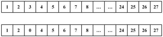
Figure 4.
Chromosome coding scheme.
- (2)
- Population initialization
The population initialization of the GA can be carried out in a variety of ways, and a common practice is to generate a number of random points comparable to the population size. Due to the complexity of the optimization model, the distribution of the initial points in the search space obtained by this random generation method has great uncertainty, which can easily make the algorithm prematurely fall into the local optimum. When the quality of the initial solution is average, it also leads to a greatly extended solution time. Therefore, the distribution of initial values is homogenized using the Tent-based chaotic mapping method.
Tent chaotic mapping is a one-dimensional discrete segmented mapping method based on chaos theory, and the function image presents a “tent” shape with a relatively uniform distribution function and good correlation. The expression of this method is:
Generally, , but when , the periodic state of the system will converge quickly, leading to unsatisfactory results. Therefore, this study takes as .
The initialization of the population is carried out after obtaining the chaotic components of each optimization parameter according to the above equation.
- (3)
- Adaptation function
Since the purpose of this model is to find the scheduling solution with the lowest total cost within the set of feasible solutions, the larger the value () of the objective function, the smaller the probability that the solution should be selected, i.e., the lower the fitness should be. Therefore, the inverse of the objective function is used as the fitness function . For poor solutions that directly violate the constraints, the penalty term function is specified to be , a sufficiently large value, so that the probability of that solution being eliminated in the next round of genetics is greatly increased; otherwise .
The calculations of are:
- (4)
- Simulated annealing perturbation
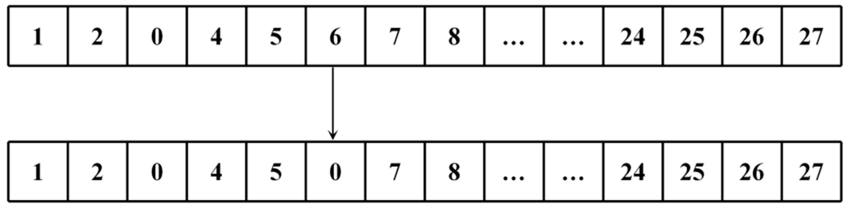
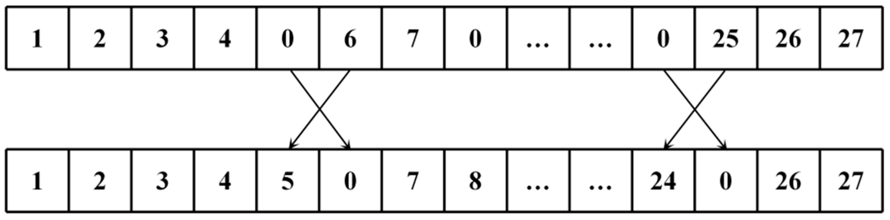
The perturbation operation in the SAA process consists of the insertion of new stop-skipping sites and the crossover swapping of stop-skipping sites in the original path. Figure 5 represents the perturbation process of random insertion, which selects any site in the parent chromosome whose gene locus value is not 0 and assigns it to 0. Figure 6 represents the perturbation process of cross-swapping, which selects two neighboring gene loci in the parent chromosome to be coded and swapped. Both perturbation operations are used simultaneously and the other gene sites that are not perturbed are retained by the offspring in the coding order of the original parent chromosome.
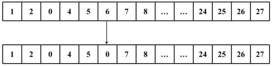
Figure 5.
Random insertion perturbation.
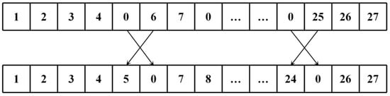
Figure 6.
Cross-swapping perturbation.
- (5)
- Selection, crossover, and mutation
A roulette approach based on an elite selection strategy is used for operator selection. The roulette strategy converts the fitness value of an individual into a selection probability, and then selects individuals based on this selection probability, where the probability of each individual being selected is the fitness value of the individual divided by the sum of the fitness of all the individuals, as shown in Figure 7. Subsequently, a range of random numbers and the corresponding individuals are selected according to the corresponding range. This procedure is repeated until the number of selected individuals reaches the preset value.
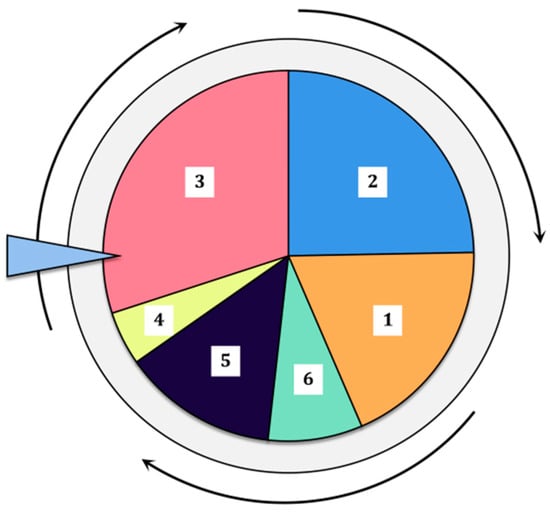
Figure 7.
Roulette selection principle. 1 to 6 represent 6 individuals, and the size of the sector represents the probability that each individual will be selected.
If the population size is , the probability that individual whose fitness is , is selected can be expressed as:
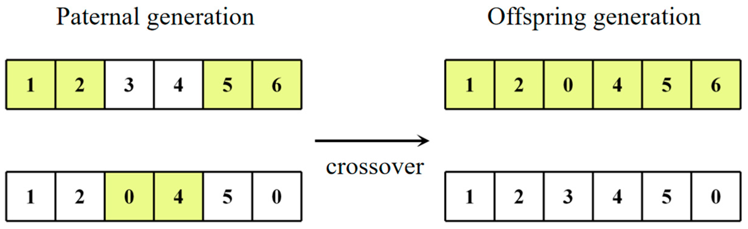
A two-point crossover is used to achieve the segment swapping of the parent chromosomes, as shown in Figure 8. The crossover operation allows the algorithm to perform a wider search in the search space and helps to find a better solution. Firstly, two crossover gene sites are randomly selected, and the two paternal individuals are cut at these two crossover points. Then, the two cut segments are interchanged and fused to obtain a new offspring individual. The fragment lengths and cutting positions are determined by the chosen loci and are, therefore, equally random, increasing the direction of evolution as much as possible while preserving the advantages of the parents.
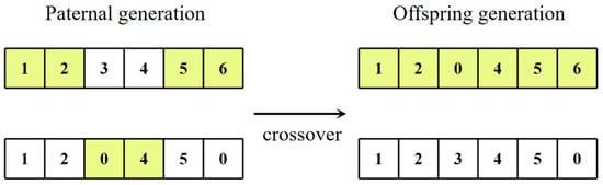
Figure 8.
Two-point crossover operation. The yellow and white blocks respectively represent segments that have been cut down and fused together from the parental generation to the offspring generation.
Common genetic mutation operations include point mutations, insertions, deletions, swapping, inversions, etc. In this study, an adaptive-mutation-rate-based mutation operation was used. Select a certain number of offspring individuals in the new population generated by the crossover completion, and calculate the mutation probability of each individual as in Equation (22). Let in the offspring generation, where individual of the subgeneration has a fitness of The average fitness of all individuals is and the fitness of the optimal individual is , so the probability of adaptive variation is:
is a probability control factor to avoid excessive variability.
For individuals with identified mutations, two gene loci in the segment were randomly selected to produce mutations. The mutation rule is that, when the value of the original gene locus is 0, the value of the mutated gene locus is 1; when the value of the original gene locus is 1, the value of the mutated gene locus is 0.
- (6)
- Algorithm termination conditions
The hybrid algorithm terminates when it reaches the upper limit of the specified number of iterations.
4. Case Study
4.1. Data Description
The basic data are the actual bus operation data of the No. 115 bus line provided by the Ganzhou Public Transportation Corporation on 28 March 2022 (Monday), including passenger flow data, on-board real-time GPS data, travel logs, and urban road network structure and coordinates. The data for each bus stops of the No. 115 bus line is shown in Table 2.
Table 2.
Bus stop coordinates and station spacing for No. 115 bus line.
4.2. Parameter Setting
In order to balance the algorithm solution speed, stability, and the feasibility of the searched optimal solution, the key parameters of the hybrid algorithm are shown in Table 3.
Table 3.
Algorithm parameter settings.
The other parameters involved in the model and solution process were set as shown in Table 4.
Table 4.
Other related parameter settings.
4.3. Analysis of Results
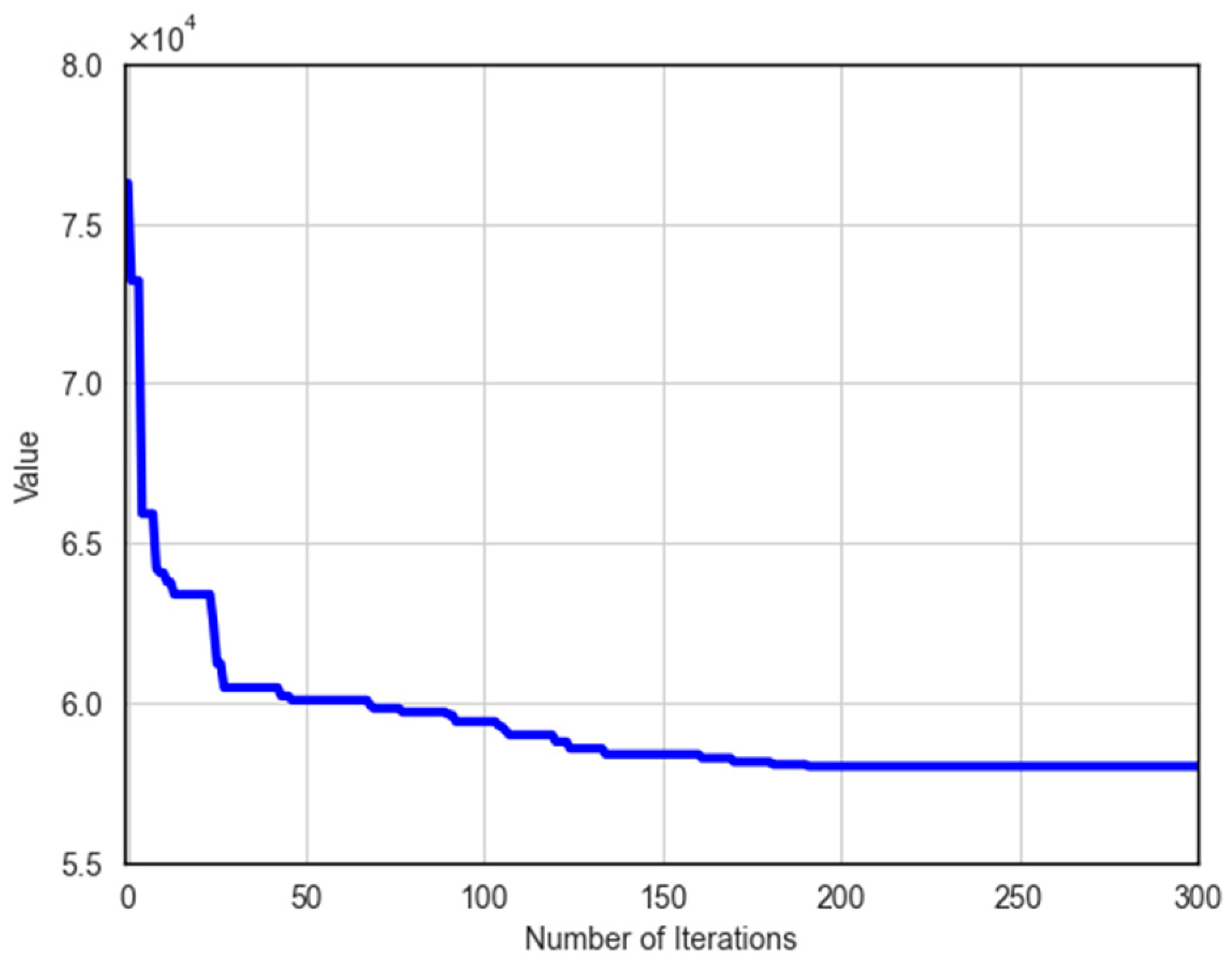
In order to validate the solution algorithm, a hybrid genetic algorithm and conventional genetic algorithm are used to solve the problem separately. Compared to the hybrid genetic algorithm, the conventional genetic algorithm does not perform operations such as simulated annealing perturbation and probabilistic reception of the solution, and the other parameters are kept the same as in the hybrid genetic algorithm compared to the hybrid algorithm. The convergence curves of the fitness functions of the two algorithms are shown in Figure 9 and Figure 10.

Figure 9.
Convergence curve of the hybrid algorithm.
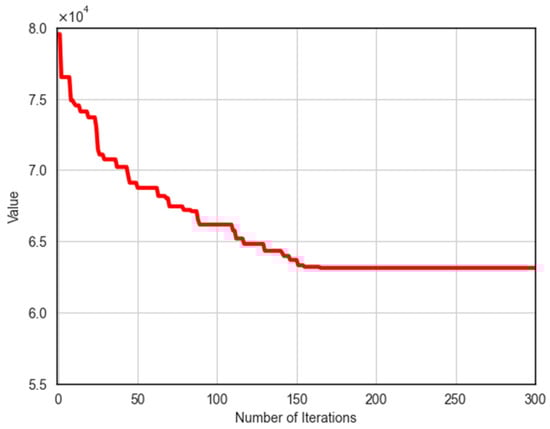
Figure 10.
Convergence curve of conventional genetic algorithm.
Comparing the two figures, it can be seen that both algorithms can iterate to obtain the optimal solution of the problem within the maximum number of iterations. From the iteration speed, the starting convergence speed of the hybrid algorithm is significantly improved compared with the conventional genetic algorithm, and the objective function value decreases rapidly within 30 generations. Then, the convergence rate decreases and converges to the optimal value in about 200 generations. From the quality of the solution, the optimal solution obtained by the conventional genetic algorithm is 8.81% higher than that of the hybrid algorithm, indicating that the simulated annealing perturbation operation can be used to make the algorithm eliminate the interference of the local optimal solution to a certain extent, thus obtaining a better evolutionary direction by accepting part of the inferior solution actively and after the cross-variation. At 50 generations, the solution obtained by the hybrid algorithm is better than the final optimization result of the conventional genetic algorithm, proving that the algorithm has a good practicability in solving this kind of problem.
In the optimal scheduling scheme calculated by the hybrid algorithm, the number of bus departures on a single day of the line is 65, and the total cost is CNY 58,144.2. As an example, in the upward direction, the results of the final calculation of the vehicle time-sharing interval and the hybrid algorithm output of the optimal vehicle scheduling program are transformed into the form shown in Table 5.
Table 5.
Optimal bus scheduling scenarios from hybrid algorithms.
In terms of service capacity, the original total passenger flow of the line in a single day is 5980 and the actual service flow of the program is 5919, with a full-day comprehensive service rate of 98.98%, which is in line with the constraints of the model and the actual operational scenarios. In terms of travel speed, the original scheduling plan has an average speed of 19.7 km/h for the whole day and 18.1 km/h for the peak period, while the optimized scheduling plan has an average speed of 21.6 km/h for the whole day and 20.3 km/h for the peak period, which are improvements of 9.64% and 12.15%. In terms of passengers, the average waiting time for passengers during the whole day is reduced by about 11.07% and the average waiting time for passengers during the peak period is reduced by about 22.15%. Due to the increase in the speed of the buses, the passengers’ traveling time will also be shortened.
In order to further analyze and evaluate the specific effects of the bus control strategy proposed in this paper, the specific scheduling scheme of some of the buses undergoing stop-skipping or route adjustment is shown in Table 6.
Table 6.
Bus operation program for the implementation of dynamic dispatching means.
Analyzing the data in the above table, the following conclusions can be drawn:
- (1)
- The trips for which the stop-skipping control strategy was implemented were concentrated in the morning and evening peak hours, and none of the trips during the weekday peak hours were implemented. This was mainly due to the large departure interval during peak hours; if a vehicle crossed the station, the passengers at that station would incur a high cost of waiting time and penalty cost. On the other hand, the peak hour routes were densely populated, and the next vehicle would arrive soon after a vehicle crossed the station, so the total cost increase was limited and easy for passengers to accept.
- (2)
- The numbers of the bus stops that buses skipped were 5, 9, 12, 13, 19, 23, 25, and 26 (specific station names are listed in Table 2). These stops generally have low patronage, the distribution of passengers is closely related to time of day, or the spacing between stations is small and transportation conditions are poor. Therefore, decision makers can discover the problems of the line station layout through the skipping frequency of the stops in the program, so as to provide reference evidence for the relocation of original bus stops and the setting of new stops.
- (3)
- The numbers of the bus stops where buses changed route were 9 and 26. Bus stop 9 (Dragon Mall) is prone to congestion in the vicinity of the Londo Mall, but there are multiple roads to choose from, thus making it easy to find a more reasonable path. For bus stop 26 (Yunlong Garden), there are too many intersections near it, tending to make buses choose to cross the stop in the calculation process. Therefore, the results of this model can also help to identify difficult route segments, which can be used as a theoretical basis for bus operators in the path optimization of existing routes and the laying of new routes.
5. Conclusions
This paper discusses, in detail, the application scenarios and implementation modes of dynamic bus scheduling means represented by stop-skipping control and local path optimization. Based on the organic combination of multiple control strategies, a dynamic optimization model for single-line bus operations is constructed, which makes up for the shortcomings of general scheduling methods and further realizes the dynamic optimization adjustment of the local reasonable amplitude of the vehicle operation path on the basis of the traditional means of crossing stations. The results obtained from this model have a good usability, which can effectively improve the average traveling speed of buses, shorten the overall waiting time of passengers, and enhance the line operation efficiency. The implementation of the model relies on real-time data processing and transmission technologies, therefore requiring a certain level of technological development in the cities where the bus routes are located. Meanwhile, the algorithm comparison experiment shows that the introduction of the simulated annealing idea can make the conventional genetic algorithm obtain a better performance in terms of iteration speed and optimal solution quality, thus verifying the advanced nature of the hybrid algorithm. In addition, the calculation results of the model can also be used as a reference basis for the evaluation and optimization adjustment of bus lines and stations, providing auxiliary judgment for scheduling operators.
Due to the limitations of the experimental conditions and the researcher’s technical level, there are still some problems that need to be improved in further studies in the future:
- (1)
- The dynamic optimization program used in the single-route bus is mainly based on the stop-skipping control strategy. Although the example results prove that this method can effectively reduce the average travel time and waiting time of passengers, the impact of vehicle crossing on individual passengers’ willingness to ride is difficult to completely eliminate.
- (2)
- The optimization model only considered a single-line bus, but in reality, multiple lines with public routes and stops will have mutual interference with each other, affecting the optimization effect of the scheduling scheme. In the future, the interactions between other lines and this line can be considered to be included in the research scenarios for quantification and modeling, so that the model can be closer to the real operating environment and the applicability of the model can be improved.
Author Contributions
Conceptualization, X.Z. (Xuemei Zhou); methodology, H.G.; software, H.G.; validation, X.Z. (Xuemei Zhou); resources, X.Z. (Xiaochi Zhao); data curation, H.G. and B.L.; writing—original draft preparation, H.G.; writing—review and editing, X.Z. (Xuemei Zhou). All authors have read and agreed to the published version of the manuscript.
Funding
This research was funded by Natural Science Foundation of China (No. 52372318).
Institutional Review Board Statement
Not applicable.
Informed Consent Statement
Not applicable.
Data Availability Statement
The raw data supporting the conclusions of this article will be made available by the authors on request.
Conflicts of Interest
The authors declare no conflicts of interest. The funders had no role in the design of the study; in the collection, analyses, or interpretation of data; in the writing of the manuscript; or in the decision to publish the results.
References
- Hall, R.; Dessouky, M.; Lu, Q. Optimal holding times at transfer stations. Comput. Ind. Eng. 2001, 40, 379–397. [Google Scholar] [CrossRef]
- Cats, O.; Larijani, A.N.; Ólafsdóttir, Á.; Burghout, W.; Andréasson, I.J.; Koutsopoulos, H.N. Bus-Holding Control Strategies: Simulation-Based Evaluation and Guidelines for Implementation. Transp. Res. Rec. 2012, 2274, 100–108. [Google Scholar] [CrossRef]
- Muñoz, J.C.; Cortés, C.E.; Giesen, R. Comparison of Dynamic Control Strategies for Transit Operations. Transp. Res. Part C Emerg. Technol. 2013, 28, 101–113. [Google Scholar] [CrossRef]
- Cortés, C.E.; Sáez, D.; Milla, F. Hybrid Predictive Control for Real-time Optimization of Public Transport Systems Operations Based on Evolutionary Multi-objective Optimization. Transp. Res. Part C Emerg. Technol. 2010, 18, 757–769. [Google Scholar] [CrossRef]
- Daganzo, C.F.; Pilachowski, J. Reducing Bunching with Bus-to-bus Cooperation. Transp. Res. Part B Methodol. 2011, 45, 267–277. [Google Scholar] [CrossRef]
- Teng, J.; Jin, W.M. A Section-speed Guiding Method for Bus Operation Control. J. Tongji Univ. (Nat. Sci.) 2015, 43, 1194–1199. [Google Scholar] [CrossRef]
- He, S.X. An Anti-bunching Strategy to Improve Bus Schedule and Headway Reliability by Making Use of the Available Accurate Information. Comput. Ind. Eng. 2015, 85, 17–32. [Google Scholar] [CrossRef]
- Estrada, M.; Mensión, J.; Aymamí, J.M. Bus Control Strategies in Corridors with Signalized Intersections. Transp. Res. Part C Emerg. Technol. 2016, 71, 500–520. [Google Scholar] [CrossRef]
- Yang, M.; Sun, G.; Wang, W.; Sun, X.; Ding, J.; Han, J. Evaluation of the Pre-detective Signal Priority for Bus Rapid Transit: Coordinating the Primary and Secondary Intersections. Transport 2018, 33, 41–51. [Google Scholar] [CrossRef]
- Ma, W.; Yang, X.; Liu, Y. Development and Evaluation of a Coordinated and Conditional Bus Priority Approach. Transp. Res. Rec. 2010, 2145, 49–58. [Google Scholar] [CrossRef]
- Anderson, P.; Daganzo, C.F. Effect of Transit Signal Priority on Bus Service Reliability. Transp. Res. Part B Methodol. 2020, 132, 2–14. [Google Scholar] [CrossRef]
- Cvijovic, Z.; Zlatkovic, M.; Stevanovic, A.; Song, Y. Conditional Transit Signal Priority for Connected Transit Vehicles. Transp. Res. Rec. 2022, 2676, 490–503. [Google Scholar] [CrossRef]
- Chandrasekar, P.; Long, C.R.; Chin, H.C. Simulation Evaluation of Route-based Control of Bus Operations. J. Transp. Eng. 2002, 128, 519–527. [Google Scholar] [CrossRef]
- Sun, A.; Hickman, M. The Real-time Stop-skipping Problem. J. Intell. Transp. Syst. 2005, 9, 91–109. [Google Scholar] [CrossRef]
- Delgado, F.; Munoz, J.C.; Giesen, R. Real-time Control of Buses in A Transit Corridor Based on Vehicle Holding and Boarding Limits. Transp. Res. Rec. 2009, 2090, 59–67. [Google Scholar] [CrossRef]
- Daganzo, C.F. A Headway-based Approach to Eliminate Bus Bunching: Systematic Analysis and Comparisons. Transp. Res. Part B Methodol. 2009, 43, 913–921. [Google Scholar] [CrossRef]
- Delgado, F.; Munoz, J.C.; Giesen, R. How Much Can Holding and/or Limiting Boarding Improve Transit Performance? Transp. Res. Part B Methodol. 2012, 46, 1202–1217. [Google Scholar] [CrossRef]
- Xuan, Y.; Argote, J.; Daganzo, C.F. Dynamic Bus Holding Strategies for Schedule Reliability: Optimal Linear Control and Performance Analysis. Transp. Res. Part B Methodol. 2011, 45, 1831–1845. [Google Scholar] [CrossRef]
- Bartholdi, J.J.; Eisenstein, D.D. A Self-Coordinating Bus Route to Resist Bus Bunching. Transp. Res. Part B Methodol. 2012, 46, 481–491. [Google Scholar] [CrossRef]
- Zheng, S.Y. Research on Public Transit Real-time Scheduling Method under the Condition of V2V Communication. Master’s Thesis, Beijing Jiaotong University, Beijing, China, 2016. [Google Scholar]
- Konstantinos, G. Stop-skipping in Rolling Horizons. Transp. A Transp. Sci. 2021, 17, 492–520. [Google Scholar] [CrossRef]
- Chen, C.X.; Chen, Z.Y.; Chen, W.Y. A Real-time Control Method for Single Bus Line Based on Fuzzy Logic. J. Highw. Transp. Res. Dev. 2016, 33, 141–147. [Google Scholar] [CrossRef]
- Zhao, J.; Bukkapatnam, S.; Dessouky, M.M. Distributed Architecture for Real-time Coordination of Bus Holding in Transit Networks. IEEE Trans. Intell. Transp. Syst. 2003, 4, 43–51. [Google Scholar] [CrossRef]
- Cats, O.; Larijani, A.N.; Koutsopoulos, H.N. Impacts of Holding Control Strategies on Transit Performance: Bus Simulation Model Analysis. Transp. Res. Rec. 2011, 2216, 51–58. [Google Scholar] [CrossRef]
- Sáez, D.; Cortés, C.E.; Milla, F. Hybrid Predictive Control Strategy for a Public Transport System with Uncertain Demand. Transportmetrica 2012, 8, 61–86. [Google Scholar] [CrossRef]
- Zhang, H.; Liang, S.D.; Zhao, J.; He, S.X.; Zhao, T.Y. Coordinated Headway-Based Control Method to Improve Public Transit Reliability considering Control Points Layout. J. Adv. Transp. 2020, 2020, 3236841. [Google Scholar] [CrossRef]
- Foletta, N.; Estrada-Romeu, M.; Roca-Riu, M. New Modifications to Bus Network Design Methodology. Transp. Res. Rec. 2010, 2197, 43–53. [Google Scholar] [CrossRef]
- Joaquín, A.P.; Caballero, R.; Laguna, M. Bi-Objective Bus Routing: An Application to School Buses in Rural Areas. Transp. Sci. 2013, 47, 397–411. [Google Scholar] [CrossRef]
- Fan, W.; Machemehl, M. Bi-Level Optimization Model for Public Transportation Network Redesign Problem. Transp. Res. Rec. 2011, 2263, 151–162. [Google Scholar] [CrossRef]
- Muhammad, A.N.; Rahman, M.K.; Rahman, M.S. Transit network design by genetic algorithm with elitism. Transp. Res. Part C Emerg. Technol. 2014, 46, 30–45. [Google Scholar] [CrossRef]
- Wang, Y.; Du, B.W.; Rong, Q.N.; Lin, X. Travel Patterns Analysis of Urban Residents Using Automated Fare Collection System. Chin. J. Electron. 2016, 25, 4047. [Google Scholar] [CrossRef]
- Bagloee, S.A.; Ceder, A. Transit-network Design Methodology for Actual-size Road Networks. Transp. Res. Part B Methodol. 2011, 45, 1787–1804. [Google Scholar] [CrossRef]
- Xiong, J.; Guan, W.; Huang, A.L. Research on Optimal Routing of Community Shuttle Connect Rail Transit Line. J. Transp. Syst. Eng. Inf. Technol. 2014, 14, 166–173. [Google Scholar] [CrossRef]
- Zhang, Y. Time-Constrained Routing Optimization Models and Algorithms under Uncertain Travel Times. Master’s Thesis, Dongbei University, Shenyang, China, 2017. [Google Scholar]
- Yu, L.J.; Zhu, Y.Z.; Yu, Z.Q.; Li, X.; Liu, W. Optimal Design for Trunk-and-feeder Bus Transit Tree Network with Heterogeneous Demand. China J. Highw. Transp. 2021, 34, 139–156. [Google Scholar] [CrossRef]
- Lin, J.J.; Wong, H.I. Optimization of a Feeder-bus Route Design by Using a Multiobjective Programming Approach. Transp. Plan. Technol. 2014, 37, 430–449. [Google Scholar] [CrossRef]
- Lyu, Y.; Chow, C.Y.; Lee, V.C.S. CB-Planner: A Bus Line Planning Framework for Customized Bus Systems. Transp. Res. Part C Emerg. Technol. 2019, 101, 233–253. [Google Scholar] [CrossRef]
- Huang, D.; Gu, Y.; Wang, S. A Two-phase Optimization Model for the Demand-responsive Customized Bus Network Design. Transp. Res. Part C Emerg. Technol. 2020, 111, 1–21. [Google Scholar] [CrossRef]
- Ma, C.; Wang, C.; Xu, X. A Multi-Objective Robust Optimization Model for Customized Bus Routes. IEEE Trans. Intell. Transp. Syst. 2021, 22, 2359–2370. [Google Scholar] [CrossRef]
- Shen, C.; Yao, S.; Bai, Z. Real-time Customized Bus Routes Design with Optimal Passenger and Vehicle Matching Based on Column Generation Algorithm. Phys. A Stat. Mech. Its Appl. 2021, 571, 125836. [Google Scholar] [CrossRef]
- Dunbar, M.; Simon, B.; Nagesh, S. A Genetic Column Generation Algorithm for Sustainable Spare Part Delivery: Application to the Sydney DropPoint Network. Ann. Oper. Res. 2020, 290, 923–941. [Google Scholar] [CrossRef]
- Qiu, G. Research on Optimizing Design Method of Customized Bus Route Based on Passenger Travel Mode Choice. Master’s Thesis, Beijing Jiaotong University, Beijing, China, 2019. [Google Scholar]


Disclaimer/Publisher’s Note: The statements, opinions and data contained in all publications are solely those of the individual author(s) and contributor(s) and not of MDPI and/or the editor(s). MDPI and/or the editor(s) disclaim responsibility for any injury to people or property resulting from any ideas, methods, instructions or products referred to in the content. |
© 2024 by the authors. Licensee MDPI, Basel, Switzerland. This article is an open access article distributed under the terms and conditions of the Creative Commons Attribution (CC BY) license (https://creativecommons.org/licenses/by/4.0/).