A Study on the Mechanical Resonance Frequency of a Piezo Element: Analysis of Resonance Characteristics and Frequency Estimation Using a Long Short-Term Memory Model

Abstract

In an ultrasonic system, a piezoelectric transducer (PT) is a key component and contains a piezo element inside. In order to design and operate a system that uses a piezo element for its intended purpose, resonance analysis of the piezo element and an equivalent circuit analysis of the output stage of the ultrasonic system generator are required. Due to the characteristics of the equivalent circuit, a piezo element has multiple resonance points. Therefore, the system must be operated at the corresponding frequency by tracking the resonance frequency that suits the purpose of the system. In this study, the mechanical resonance frequency of the piezo element was analyzed and a method for operating the system at the corresponding frequency was studied. In order to operate a piezo element, a voltage-type inverter is used to apply a high-frequency AC (Alternating Current). Then, an $LC$ filter is inserted into the output stage of the inverter, and the piezo element is finally located at the output stage of the $LC$ filter. Therefore, when designing an $LC$ filter, a design is required to optimize the performance of the piezo element. In this paper, we analyzed the resonance of a piezo element and the equivalent circuit of the generator output stage of an ultrasonic system for effective operation of an ultrasonic system. In addition, we proposed a method to estimate the characteristics of the entire mechanical resonance frequency range of a piezo element by using an LSTM (Long Short-Term Memory) model suitable for analyzing the nonlinear characteristics of a piezo element. The study on estimating the mechanical resonance frequency of a piezo element using an LSTM model was verified through MATLAB 2021b simulation and ultrasonic system experiments.

1. Introduction

The output of the ultrasonic system includes a piezo element that converts electrical energy into mechanical energy and vibration [1,2]. When operating an ultrasonic system whose main purpose is mechanical energy conversion, the system must be operated at the mechanical resonance frequency of the piezo element [3]. This is because the mechanical structure of the piezo element vibrates most effectively at that frequency, generates the largest displacement, and has high energy conversion efficiency. However, the mechanical resonance frequency of the piezo element varies depending on the load and external environment. Therefore, in order to maintain a stable output in the ultrasonic system, it is essential to operate the system at the resonance frequency. In order to generate mechanical vibration in the piezo element, a high-frequency AC sine wave must be applied [4,5]. For this reason, it is common to use a voltage-type inverter and configure the system by inserting various types of $LC$ filters into the inverter output [6,7,8]. In addition, the R, L, and C parameter values inside the piezo element vary depending on external conditions, such as pressure, temperature, and operating status [9,10,11]. As there are many parameter factors to consider when operating an ultrasonic system, the field related to the resonance point of the piezo element is currently being much studied. The existing general ultrasonic system operation methods are to operate the entire system at the resonance frequency, including the $LC$ filter of the ultrasonic system inverter output stage and the parallel capacitor in the piezo element equivalent circuit [12,13,14]. The parallel capacitor in the piezo element equivalent circuit affects the anti-resonance frequency [15,16]. Therefore, in order to operate the system at the mechanical resonance frequency of the piezo element, it is necessary to consider the influence of the parasitic capacitor in the piezo element equivalent circuit model. In this paper, we analyzed the resonance of the piezo element to effectively operate the ultrasonic system at the mechanical resonance frequency of the piezo element. The analysis contents include the characteristics of the parasitic capacitor of the piezo element, the design of the $LC$ filter, and the equivalent circuit analysis of the ultrasonic system output stage using the s-plane natural response characteristics. In addition, the LSTM model was used in MATLAB simulation to analyze the relationship between the resonance frequency of the ultrasonic system output stage and the mechanical resonance frequency of the piezo element [17,18]. Research on predicting the frequency step of the system or modeling and predicting various dynamic processes using the LSMT model is currently being actively conducted. In the study of ‘A Novel CNN-LSTM Hybrid Model for Prediction of Electro-Mechanical Impedance Signal Based Bond Strength Monitoring’ by Lukesh Parida [19], a hybrid model combining a CNN (Convolutional Neural Network) and LSTM was used to perform structural basis signature prediction. In particular, as a case used to predict the resonance frequency, the frequency step was predicted from the data of the EMI (Electro-Mechanical Impedance) signature. In the study ‘CNN-LSTM deep learning architecture for computer-vision-based modal frequency detection’ by Ruoyu Yang [20], a new approach utilizing computer vision and deep learning was proposed to overcome the shortcomings of traditional vibration analysis methods. In particular, a deep learning model combining a CNN and LSTM was proposed to solve the problem, and the vibration frequency of the structure was extracted by receiving the camera image as input in a non-contact manner. As a result, it showed higher accuracy than the existing vibration measurement technology and could operate more efficiently and autonomously. As shown above, compared to the existing method, the LSTM model enables effective analysis in a system that predicts or extracts nonlinear frequencies. Since the piezo element has nonlinear characteristics, an LSTM model suitable for it was used, and a method for estimating the characteristics of the entire mechanical resonance frequency range of the piezo element was proposed in this paper. Finally, the mechanical resonance frequency of the piezo element was estimated using the LSTM model, and the system was operated at the corresponding frequency to verify this experimentally.

2. Analysis of Piezo Element

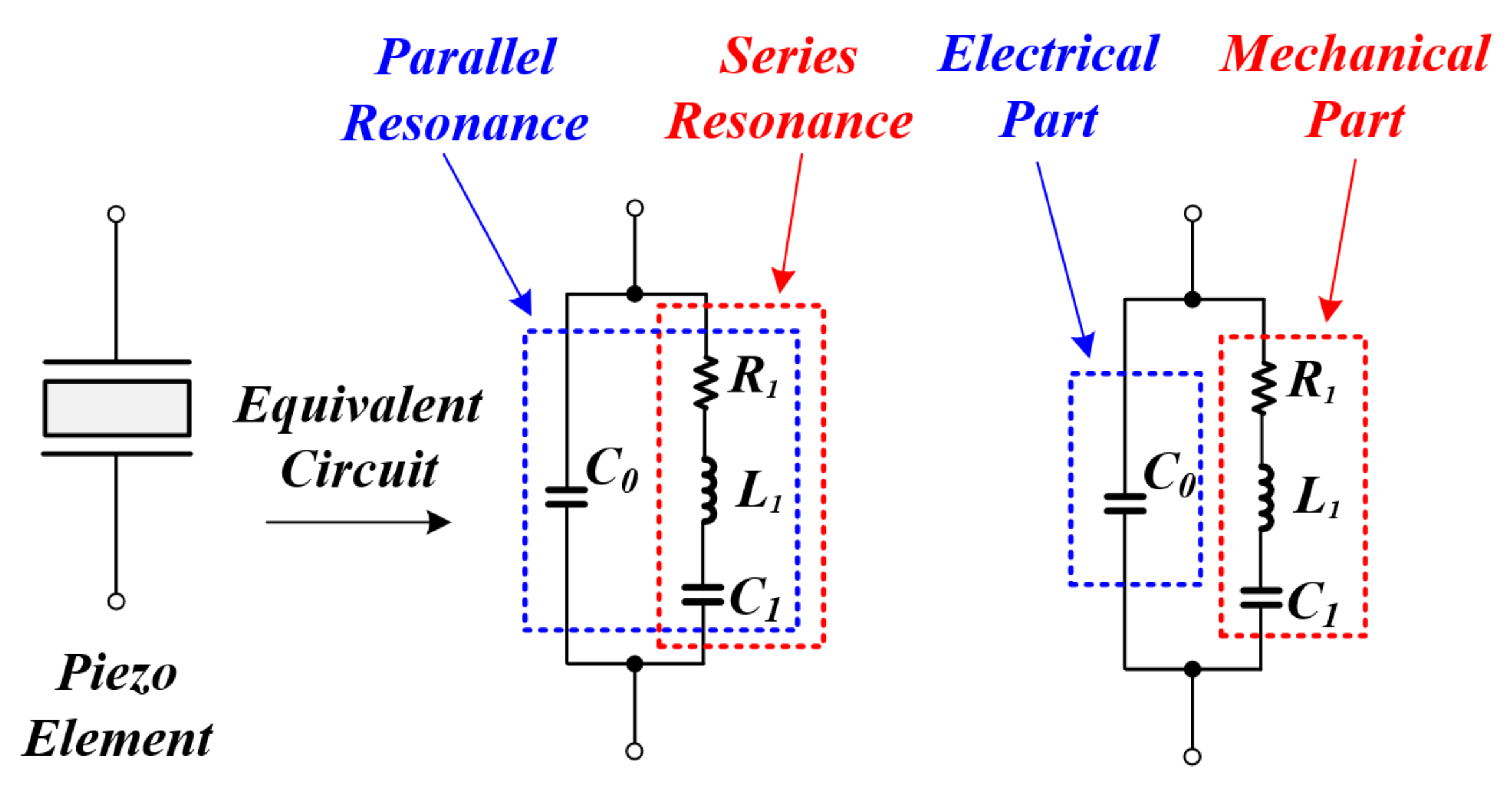
2.1. Equivalent Circuit Model Analysis and Resonance Characteristics of Piezo Element

The piezo element can be expressed as an equivalent model consisting of the $R_1$$L_1$$C_1$ series circuit part that affects the mechanical output and the parasitic capacitor $C_0$, as shown in Figure 1. The first arm is an electrical arm that includes the parasitic capacitor $C_0$, and the other arm is a mechanical arm consisting of the dynamic capacitor $C_1$, the dynamic inductor $L_1$, and the dynamic resistor $R_1$. As can be seen from the equivalent model above, the piezo element has a structure with two resonance points, as shown in the equation below as (1), (2) [21,22].

$$f_r={\displaystyle \frac{1}{2\pi \sqrt{L_1{C}_1}}}$$

(1)

$$f_a={\displaystyle \frac{1}{2\pi \sqrt{L_1\left(\frac{C_1{C}_0}{C_1+C_0}\right)}}}$$

(2)

The resonant frequency ($f_r$) of the $R_1$$L_1$$C_1$ series circuit of the mechanical arm is organized as in (1), and this becomes the mechanical resonant frequency that delivers the maximum power to the piezo element. And, the total resonant frequency ($f_a$) of the piezo element including the parasitic capacitor $C_0$ is organized as in (2). In other words, the piezo element exists in a form where both the resonant frequency and the anti-resonant frequency exist due to the influence of the parasitic capacitor $C_0$. Therefore, if the system is operated with an incorrect resonant frequency, the output may not be properly delivered to the piezo element due to the influence of the anti-resonant frequency. Therefore, in order to accurately deliver the output to the piezo element, the system must be operated with the mechanical resonant frequency ($f_r$), such as (1), that can deliver the maximum power [23,24,25].

The following is the change characteristics of piezo element parameters according to pressure fluctuation. In general, piezo elements have the characteristic that internal parameter values fluctuate according to changes in external conditions (pressure, temperature, etc.), and Figure 2 shows the piezo element parameter values according to pressure fluctuation. Since each parameter value fluctuates according to pressure fluctuation, the mechanical resonance frequency of the piezo element also fluctuates. However, the parasitic capacitor $C_0$ value is almost constant regardless of pressure fluctuation. This can be interpreted as the effect of the resonance frequency fluctuation due to the parasitic capacitor $C_0$ value being very small compared to the resonance frequency fluctuation due to the series $R_1$$L_1$$C_1$ value. Therefore, if the system is designed so that the effect of the parasitic capacitor $C_0$ can be ignored when designing the $LC$ filter of the inverter output stage in the ultrasonic system, the resonance frequency fluctuation of the piezo element will be even smaller. As a result, the entire equivalent model of the ultrasonic system can be newly interpreted by separating it into two major impedances: the $R_1$$L_1$$C_1$ series circuit and the $LC$ filter, which affect the mechanical output from the piezo element.

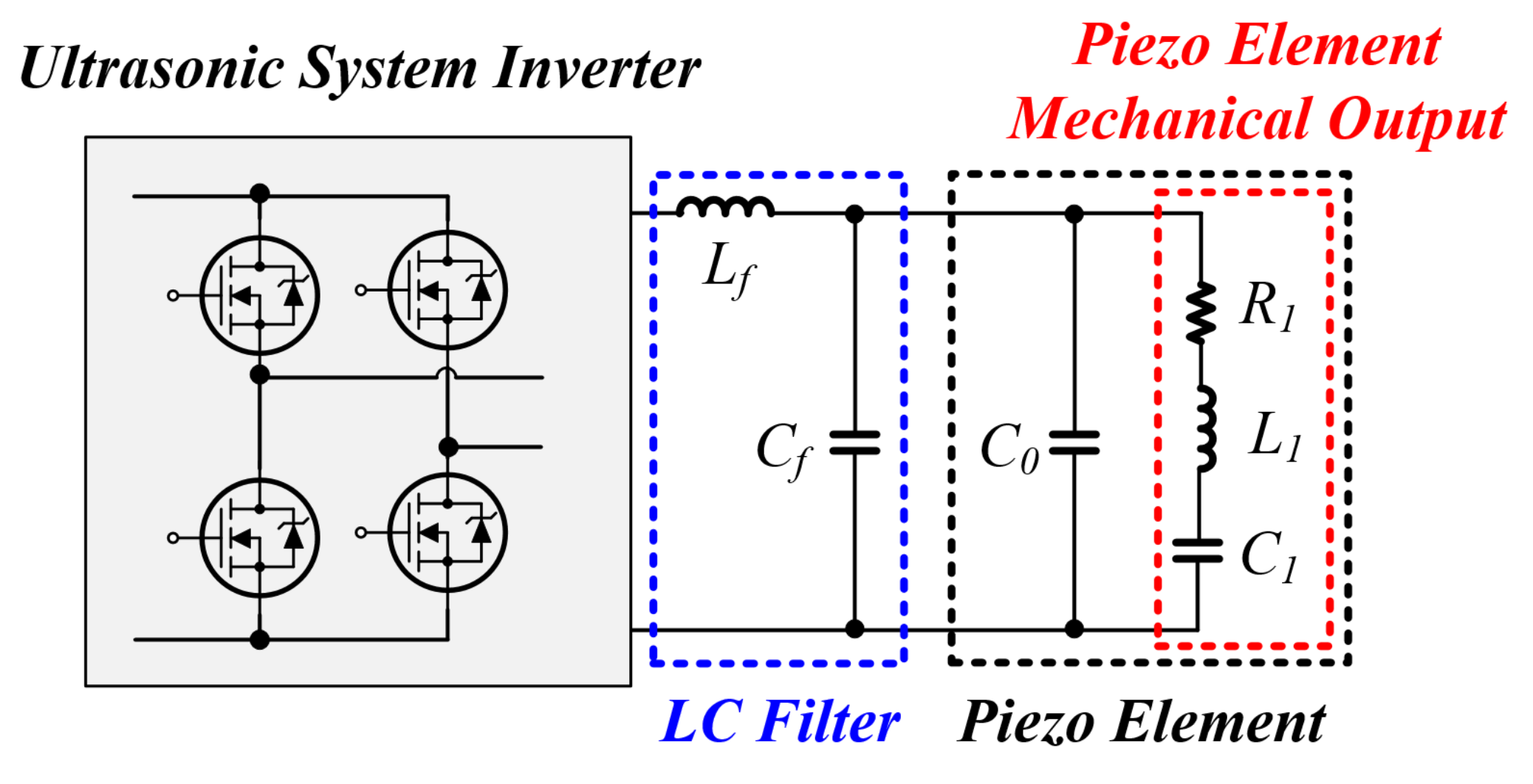
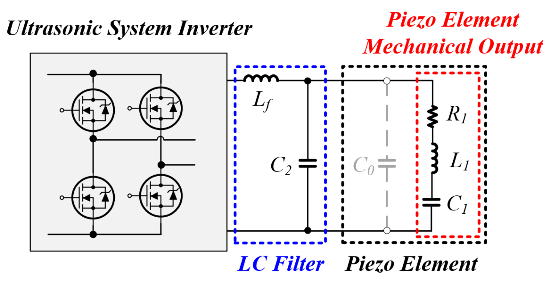
2.2. Equivalent Circuit Analysis of the Ultrasonic System Output Stage

Figure 3 is the equivalent circuit of the inverter output stage in the ultrasonic system, and can be interpreted as the equivalent circuit of the entire system. As shown in Figure 3, the parasitic capacitor $C_0$ of the piezo element and the capacitor $C_f$ of the $LC$ filter are connected in parallel, so they can be considered as one capacitor $C_2$. Since $L_f$ and $C_f$ of the $LC$ filter are values designed by the user, they are fixed values that do not change, and the parasitic capacitor $C_0$ of the piezo element has very little change in value and is almost constant [13,26,27,28,29].

Accordingly, if the filter $C_f$ value is designed to be sufficiently high enough to ignore the influence of the parasitic capacitor $C_0$, it can be separated into two parts: the $R_1$$L_1$$C_1$ series circuit impedance that affects the mechanical output of the piezo element and the impedance of the $LC$ filter, as shown in Figure 4. The parameter value change of the capacitor $C_2$ according to the pressure fluctuation of the piezo element is as shown in Figure 2, and the value fluctuation is very small to the extent that it hardly affects the resonant frequency of the piezo element. As a result, it can be separated into two parts: the $R_1$$L_1$$C_1$ series circuit impedance that affects the mechanical output of the piezo element and the impedance of the $LC$ filter [30].

To analyze the entire system impedance, each impedance $Z_1$, $Z_2$, and $Z_p$ is represented as in Figure 5, and the formula for this is as follows.

$L_1$, $L_f$ reactance and $C_1$, $C_2$ reactance are as follows:

$$\begin{array}{c}\hfill X_{L1}=w{L}_1,X_{C1}=-{\displaystyle \frac{1}{w{C}_1}}\\ \hfill X_{Lf}=w{L}_f,X_{C2}=-{\displaystyle \frac{1}{w{C}_2}}\end{array}$$

(3)

The piezo element $R_1$ + $L_1$ + $C_1$ total $Z_p$ impedance is as follows:

$$\begin{array}{c}\hfill Z_p=R_1+j{X}_{L1}+j{X}_{C1}\\ \hfill =R_1+j(X_{L1}+X_{C1})\end{array}$$

(4)

The $Z_1$ parallel impedance, excluding the filter $L_f$ impedance, is as follows:

$$\begin{array}{cc}\hfill Z_1& ={\displaystyle \frac{Z_p\times j{X}_{C2}}{Z_p+j{X}_{C2}}}\hfill \\ \hfill & ={\displaystyle \frac{(R_1+j(X_{L1}+X_{C1}))\times j{X}_{C2}}{(R_1+j(X_{L1}+X_{C1}))+j{X}_{C2}}}\hfill \\ \hfill & ={\displaystyle \frac{-X_{L1}{X}_{C2}-X_{C1}{X}_{C2}+jR{X}_{C2}}{R+j(X_{L1}+X_{C1}+X_{C2})}}\hfill \end{array}$$

(5)

$Z_p$ is the series $R_1$$L_1$$C_1$ impedance of the piezo element, and $Z_1$ is the sum capacitor $C_2$ of the parallel capacitor $C_0$ of the piezo element and the capacitor $C_f$ of the $LC$ filter, so it can be expressed as (5) above. Through this, the entire system impedance $Z_2$, including the inductor $L_f$ of the $LC$ filter, can be expressed as (6) below.

The total equivalent impedance $Z_2$, including the inductor $L_f$ of the $LC$ filter, is as follows:

$$\begin{array}{cc}\hfill Z_2& ={\displaystyle \frac{-X_{L1}{X}_{C2}-X_{C1}{X}_{C2}+jR{X}_{C2}}{R+j(X_{L1}+X_{C1}+X_{C2})}}+j{X}_{Lf}\hfill \end{array}$$

(6)

As shown in (6), once the values of the $LC$ filter components $L_f$ and $C_f$ are determined along with the series $R_1$$L_1$$C_1$ values of the piezo element, the resonant impedance of the entire system, including both the $LC$ filter and the piezo element, can be analyzed.

When voltage is initially applied to an ultrasonic system, a transient phenomenon occurs due to the exchange of magnetic energy and electrostatic energy of the inductor and capacitor configured in the circuit. This can be derived as a characteristic equation that represents the unique characteristics of the actual system, and the natural response characteristics can be confirmed through the roots derived from the characteristic equation, which are called characteristic roots. The characteristic roots determine the response characteristics of the circuit according to the values of the damping frequency and resonant frequency. In general, the characteristics of piezo elements exhibit under-damping characteristics due to the characteristic that the damping frequency is lower than the resonant frequency, and, in this study, the resonant frequency was analyzed through this characteristic. The resonant frequency at this time means the entire system resonant frequency of the ultrasonic system output terminal. The characteristic equation of the equivalent circuit as shown in Figure 4 is as follows.

$$\begin{array}{cc}\hfill H_{\left(fig4\right)}\left(s\right)& ={\displaystyle \frac{C_0{C}_1{L}_0{L}_1(C_1{L}_1{s}^2+C_1{R}_{1}s+1)}{C_0{C}_1{L}_0{L}_1{s}^4+C_0{C}_1{L}_0{R}_1{s}^3+(C_0{L}_0+C_1{L}_0+C_1{L}_1)s^2+C_1{R}_{1}s+1}}\hfill \end{array}$$

(7)

The characteristic equation of a fourth-order system, as described above, is very complex and difficult to solve for characteristic roots. Therefore, the response characteristics of the circuit can be analyzed using the s-plane, as shown in Figure 6.

As shown in Figure 6 above, there are poles with different real part sizes and frequency characteristics in the s-plane due to the transfer function of the fourth-order system [31,32]. At this time, if the real part ($\alpha 2$) of the pole located farther from the imaginary part among the two poles is 5 to 10 times larger than the real part ($\alpha 1$) of the pole closer to the imaginary part, it can be distinguished as a dominant pole and an insignificant pole [33]. In general, the transient response characteristics of the insignificant pole show fast damping while the dominant pole has a characteristic of relatively slow damping, and the characteristics of this are shown in Figure 7. Using these characteristics, we tried to detect the entire system resonance frequency of the ultrasonic system and find the mechanical resonance frequency of the piezo element through this. The proposed resonance frequency tracking method is summarized as follows. When voltage is applied to the ultrasonic system, a transient phenomenon in the form of under-braking occurs due to the exchange of the magnetic energy and electrostatic energy of the inductor and capacitor [30]. At this time, the transient phenomenon of the fourth-order system applied in this system appears with the damping characteristics and resonance frequency due to the dominant and insignificant poles. After the damping of the insignificant pole with relatively fast damping characteristics is completely achieved, only the damping characteristics and resonance frequency due to the dominant pole exist. At this time, the resonance frequency refers to the resonance frequency due to the inductor and capacitor components included in the entire ultrasonic system. In addition, the resonance frequency of the entire system according to the parameter value change of the piezo element was simulated and verified, and the mechanical resonance frequency of the piezo element was found through this. The resonance frequency of the entire system of the ultrasonic system output stage and the mechanical resonance frequency of the piezo element can be analyzed through a mathematical formula, Equation (6) mentioned above, and the characteristic equation calculation. This process consists of calculating the characteristic equation, calculating the characteristic root, calculating the damping period and the vibration period, and calculating the resonant frequency. The following are the formulas for the ultrasonic system output terminal and the piezo element.

Entire Ultrasonic System

$$H_{\mathrm{total}}\left(s\right)={\displaystyle \frac{C_0{C}_1{L}_f{L}_1{s}^4+C_1{L}_1{s}^2+1}{C_0{C}_1{L}_f{L}_1{s}^4+C_0{C}_1{L}_f{R}_1{s}^3+(C_0{L}_f+C_1{L}_f+C_1{L}_1)s^2+C_1{R}_{1}s+1}}$$

(8)

$$C_0{C}_1{L}_f{L}_1{s}^4+C_0{C}_1{L}_f{R}_1{s}^3+(C_0{L}_f+C_1{L}_f+C_1{L}_1)s^2+C_1{R}_{1}s+1=0$$

(9)

The characteristic roots s can generally be expressed as

$$s={\alpha }_{\mathrm{total}}\pm j{\omega }_{d,\mathrm{total}}$$

(10)

where ${\alpha }_{\mathrm{total}}$ is the damping coefficient and ${\omega }_{d,\mathrm{total}}$ is the damped natural frequency. The damping coefficient and damped natural frequency are defined as follows:

$${\alpha }_{\mathrm{total}}=-{\displaystyle \frac{R_1}{2L_1}}$$

(11)

$${\omega }_{d,\mathrm{total}}=\sqrt{{\omega }_0^2-{\alpha }_{\mathrm{total}}^2}$$

(12)

where ${\omega }_0$ is the undamped natural frequency, defined as

$${\omega }_0={\displaystyle \frac{1}{\sqrt{L_1{C}_1}}}$$

(13)

The resonant frequency $f_{\mathrm{resonance},\mathrm{total}}$ is calculated by converting the damped natural frequency ${\omega }_{d,\mathrm{total}}$ to the following frequency:

$$f_{\mathrm{resonance},\mathrm{total}}={\displaystyle \frac{{\omega }_{d,\mathrm{total}}}{2\pi }}$$

(14)

Piezo Element (Including Parasitic Capacitance $C_0$)

$$H_{\mathrm{piezo}}\left(s\right)={\displaystyle \frac{C_1{L}_1{s}^2+1}{C_1{L}_1{s}^2+(C_1+C_0)R_{1}s+1}}$$

(15)

$$C_1{L}_1{s}^2+(C_1+C_0)R_{1}s+1=0$$

(16)

The characteristic roots s can generally be expressed as

$$s={\alpha }_{\mathrm{piezo}}\pm j{\omega }_{d,\mathrm{piezo}}$$

(17)

where ${\alpha }_{\mathrm{piezo}}$ is the damping coefficient and ${\omega }_{d,\mathrm{piezo}}$ is the damped natural frequency. The damping coefficient and damped natural frequency are defined as follows:

$${\alpha }_{\mathrm{piezo}}=-{\displaystyle \frac{(C_1+C_0)R_1}{2L_1}}$$

(18)

$${\omega }_{d,\mathrm{piezo}}=\sqrt{{\omega }_0^2-{\alpha }_{\mathrm{piezo}}^2}$$

(19)

where ${\omega }_0$ is the undamped natural frequency, defined as

$${\omega }_0={\displaystyle \frac{1}{\sqrt{L_1{C}_1}}}$$

(20)

The resonant frequency $f_{\mathrm{resonance},\mathrm{piezo}}$ is calculated by converting the damped natural frequency ${\omega }_{d,\mathrm{piezo}}$ to the following frequency:

$$f_{\mathrm{resonance},\mathrm{piezo}}={\displaystyle \frac{{\omega }_{d,\mathrm{piezo}}}{2\pi }}$$

(21)

Piezo Element (Excluding Parasitic Capacitance $C_0$)

$$H_{\mathrm{no}\_\mathrm{parasitic}}\left(s\right)={\displaystyle \frac{L_1{C}_1{s}^2+1}{L_1{C}_1{s}^2+R_1{C}_{1}s+1}}$$

(22)

$$L_1{C}_1{s}^2+R_1{C}_{1}s+1=0$$

(23)

The characteristic roots s can generally be expressed as

$$s={\alpha }_{\mathrm{no}\_\mathrm{parasitic}}\pm j{\omega }_{d,\mathrm{no}\_\mathrm{parasitic}}$$

(24)

where ${\alpha }_{\mathrm{no}\_\mathrm{parasitic}}$ is the damping coefficient and ${\omega }_{d,\mathrm{no}\_\mathrm{parasitic}}$ is the damped natural frequency. The damping coefficient and damped natural frequency are defined as follows:

$${\alpha }_{\mathrm{no}\_\mathrm{parasitic}}=-{\displaystyle \frac{R_1}{2L_1}}$$

(25)

$${\omega }_{d,\mathrm{no}\_\mathrm{parasitic}}=\sqrt{{\omega }_0^2-{\alpha }_{\mathrm{no}\_\mathrm{parasitic}}^2}$$

(26)

where ${\omega }_0$ is the undamped natural frequency, defined as

$${\omega }_0={\displaystyle \frac{1}{\sqrt{L_1{C}_1}}}$$

(27)

The resonant frequency $f_{\mathrm{resonance},\mathrm{no}\_\mathrm{parasitic}}$ is calculated by converting the damped natural frequency ${\omega }_{d,\mathrm{no}\_\mathrm{parasitic}}$ to the following frequency:

$$f_{\mathrm{resonance},\mathrm{no}\_\mathrm{parasitic}}={\displaystyle \frac{{\omega }_{d,\mathrm{no}\_\mathrm{parasitic}}}{2\pi }}$$

(28)

Through the above process, the resonance frequency of the ultrasonic system output terminal and the piezo element can be analyzed. As a result, the circuit characteristics that exist in the ultrasonic system output terminal, including inductor components and capacitor components, will exhibit nonlinear characteristics. In addition, the mechanical resonance frequency of the piezo element does not have linear characteristics due to the fluctuation in the $L_1$ and $C_1$ values of the piezo element. Therefore, an algorithm that can estimate the nonlinear mechanical resonance frequency of the piezo element based on data on the ultrasonic system resonance frequency is required. In this study, a method that can estimate the characteristics of the entire mechanical resonance frequency range of the piezo element is proposed using an LSTM model suitable for analyzing the nonlinear characteristics of the piezo element. This was estimated using MATLAB simulation and the LSTM model, and the system was operated using the corresponding frequency and verified through experiments.

3. Simulation

In this chapter, MATLAB simulation was performed to analyze the relationship between the entire system resonance frequency of the ultrasonic system output stage and the mechanical resonance frequency of the piezo element. Usually, the capacitor $C_f$ value of the $LC$ filter is selected to be about 10 times larger than the parasitic capacitor $C_0$ value of the piezo element. The reason is to optimize the performance of the filter and minimize the influence of parasitic capacitance. If $C_f$ is 10 times $C_1$, the value of $C_2$ is about 1.1 times $C_f$. Therefore, the influence of the change in $C_1$ on $C_2$ is reduced to less than 10%; that is, when $C_2$ is about 1.1 times $C_f$, the change in the resonance frequency is about $\sqrt{1.1}$, which is about 5%. Based on this, the value of $C_f$ was selected as 33 nF and the simulation was performed, and the filter was designed with the corresponding value in the ultrasonic system tested in this study. In an ultrasonic system, matching the resonant frequency of the inverter output stage and the resonant frequency of the piezo element as closely as possible is an important part of the system design. When the resonant frequency of the piezo element and the resonant frequency of the inverter output match, the energy transfer efficiency is maximized. Impedance matching is also an important part, because the impedance of the piezo element is minimal at the resonant frequency, which matches well with the output impedance of the inverter. Therefore, since the $C_f$ value was determined above, the inductor Lf value that matches the corresponding value was selected as 867 $\mu$H and the simulation was conducted, and the $LC$ filter was finally designed with the corresponding values above. The MATLAB simulation conditions that considered the design details of the ultrasonic system as above are as shown in

Table 1. MATLAB simulation conditions.

Parameters	Parameter Values	Conditions
$R_1$	220 $\Omega$	-
$L_1$	190 to 240 mH	Increase by 1 mH
$C_1$	120 to 140 pF	Increase by 1 pF
$C_0$	3.25 nF	Fixed value
$L_f$	870 $\mu$H	-
$C_f$	33 nF	-
$LC$ filter resonant frequency	28.3 kHz	Filter capacitor $C_2$

below.

Although $L_1$ and $C_1$ of the piezo element are values that change depending on the pressure, the simulation was conducted by setting the parameter values for each in order to express them in the graph. However, in the graph of Figure 8, $L_1$ and $C_1$ change in a monotonically increasing pattern.

Figure 8 is an s-plane graph according to the pressure fluctuation of the piezo element. The result is that the characteristic root is plotted by assigning different colors to each $C_1$ value and maintaining the same color for the $L_1$ value. The $LC$ filter value is a fixed value determined during the design of the ultrasonic system, and the graph shows the case where the values fluctuate from $L_1$ 190 to 240 mH and $C_1$ 120 to 140 pF in the equivalent model of the piezo element. As the value of inductor $L_1$ increases, the real part value of the x-axis moves toward 0. As the value of capacitor $C_1$ increases, the imaginary part value of the y-axis moves toward 0. In the graph, blue is when the capacitor value is 120 pF, red is 130 pF, and yellow is 140 pF. And the inductor value at this time ranges from 190 to 240 mH. The range is the range of the minimum and maximum values measured at $L_1$ and $C_1$ when pressure is applied to the piezo element. As shown in Figure 8, it can be separated into the dominant and insignificant poles, and the insignificant pole showed a distribution diagram like the graph in Figure 8 according to the parameter value fluctuation of the piezo element.

Figure 9 and Figure 10 are the damping characteristic graphs of the ultrasonic system and piezo element. According to the conditions in Table 1, the characteristic equation, characteristic root, damping period, vibration period, and resonance frequency are calculated, and these are shown in the graphs of Figure 9 and Figure 10. The red graph in Figure 9 shows the output stage of the ultrasonic system, including the piezo element and $LC$ filter, and the blue graph shows the damping curve and envelope of the piezo element, excluding the parasitic capacitor $C_0$. Figure 10 shows the damping curve and envelope of the piezo element, including the $LC$ filter and parasitic capacitor $C_0$, added to Figure 9. The green color is a damping graph for the $LC$ filter only. If a simulation is performed with $L_1$ 190, 240 mH and $C_1$ 120, 140 pF, which are the minimum and maximum value ranges according to the pressure fluctuation of the piezo element, data can be obtained that can estimate the characteristics of the ultrasonic system resonance frequency and the mechanical resonance frequency of the piezo element.

Figure 11 is a graph of the relationship between the ultrasonic system resonance frequency and the piezo element mechanical resonance frequency. The data were obtained through the process of calculating the characteristic equation, calculating the characteristic root, calculating the damping period and the vibration period, and calculating each resonance frequency, and then this was displayed as a graph. The x-axis represents the entire system resonance frequency ($f_{system}$) of the ultrasonic system output stage, and the y-axis represents the piezo element mechanical resonance frequency ($f_{piezo}$). As can be seen in Figure 11, the ultrasonic system resonance frequency and the piezo element mechanical resonance frequency each have a nonlinear relationship, and it was verified that this can be analyzed by calculating the characteristic equation and the damping characteristic. The ultrasonic system resonance frequency can be seen to be divided into right and left sections based on 30 kHz due to nonlinear characteristics. In order to analyze the ultrasonic system resonance frequency, the right resonance frequency blue section was divided into 1, and the left resonance frequency pink section was divided into 2. In this study, we propose a method to estimate the optimal resonance frequency through regression analysis to maximize the mechanical output of the piezo element by measuring the frequency of the entire system combined with the input filter and the piezo element. Therefore, it is important to select a model suitable for the piezo element showing nonlinear characteristics, learn the data, and simulate them. MATLAB simulation results showed that linear regression analysis and multiple regression analysis among various machine learning models were not suitable for estimating the resonance frequency due to the nonlinear characteristics of the piezo element itself. Accordingly, we attempted to estimate the optimal resonance frequency through a nonlinear regression analysis model and LSTM regression analysis suitable for piezo elements with nonlinear characteristics. The input data for learning were the series $R_1$$L_1$$C_1$ and $L_f$ and $C_f$ of the $LC$ filter, which are responsible for the mechanical output of the piezo element. At this time, the relationship between the entire system frequency and the resonance frequency of the piezo element was estimated by inputting a monotonous increasing pattern of $L_1$ 190 to 240 mH and $C_1$ 120 to 140 pF, which affect the resonance frequency among the series $R_1$$L_1$$C_1$ of the piezo element. The verification of the learned model utilized the entire system frequency according to the load change measured in the actual system as verification data. The nonlinear regression model has the advantage of expressing the complex nonlinear relationship between input and output, so it was designed as a polynomial model considering the nonlinear characteristics of the piezo element. However, this model has limitations in solving the long-term dependency problem of time series data. To compensate for this, an LSTM regression model, which is suitable for time series data processing and effective at modeling the complex dynamic characteristics of the piezo element, was additionally designed, and experiments were conducted. The simulation conditions that considered the matters for estimating the optimal resonance frequency using the above LSTM model are as shown in

Table 2. LSTM model hyperparameters.

Parameters	Parameter Values
Input Dimension	1
Number of Hidden Units	200
Number of Epochs	200
Batch Size	100

.

The input dimension is one-dimensional data because the parameters used in the LSTM model are the ultrasonic system resonance frequency ($f_{system}$), the piezo element mechanical resonance frequency ($f_{piezo}$), the parameter values $L_1$ and $C_1$ of the piezo element, and $L_f$ and $C_f$ of the $LC$ filter. The hidden unit uses the six one-dimensional data mentioned above as input, and if the number of hidden units is too large or small, meaningful results cannot be obtained and the gradient vanishing phenomenon may occur. In this study, the number of hidden units was defined as 50, 100, 150, 200, 250, and 300, respectively, and the experiment was conducted, and the regression analysis was performed most stably when the number of hidden units was 200. In other words, this is the number of hidden units defined through the experiment based on the data learned in this study. The number of epochs was also not further trained because the learning rate did not increase after 200 or more training sessions. This may vary depending on the parameters used in the LSTM model or the results of the experiment. The number of epochs is the most optimized value for the data and experiments in this study. In other words, it may vary depending on the experimental environment (amount of data used for training, hardware status). The batch size was set to match the hardware of the system used in this study (GPU core performance and capacity) that conducted the training, and is a value determined by the experimental environment.

Figure 12 is a diagram of the LSTM model used in this experiment. The LSTM model used in the experiment is a bidirectional LSTM model consisting of one input layer, one LSTM layer, one fully connected layer, and one regression output layer. Since using two or more LSTM layers can cause the gradient vanishing problem, it was configured as one layer.

Figure 13 and Figure 14 show the results of MATLAB learning simulations to estimate the relationship between the entire system frequency and the mechanical resonance frequency of the piezo element through regression analysis using a nonlinear regression model and an LSTM model. The ultrasonic system resonance frequency on the x-axis in Figure 11 can be seen to be divided into right and left sections based on 30 kHz due to nonlinear characteristics. Therefore, the right resonance frequency section was divided into 1 and the left resonance frequency section was divided into 2, and the analysis was conducted using the LSTM model. As a result, the characteristics of the entire mechanical resonance frequency range of the piezo element were estimated using the LSTM model. Figure 13a shows the estimation of the mechanical resonance frequency of the piezo element using a nonlinear regression model for Section 1, and Figure 13b shows the estimation of the mechanical resonance frequency of the piezo element using the LSTM model, respectively. Figure 14a shows the estimation of the mechanical resonance frequency of the piezo element using the nonlinear regression model for Section 2, and Figure 14b shows the estimation of the mechanical resonance frequency of the piezo element using the LSTM model, respectively. In order to improve the learning accuracy of the two models, the min-max normalization of the data set was applied as a preprocessing step. The configuration of LSTM was set to the number of input dimensions 1, the number of hidden units 200, the number of epochs 200, and the batch size 100, as shown in Table 2. As a result of analyzing the frequency relationship, the RMSE (Root Mean Square Error) of the nonlinear regression model was 0.1922 and the RMSE of the LSTM model was 0.0124. It was confirmed that the LSTM model showed a significantly lower RMSE value than the nonlinear regression model, providing more precise results for estimating the resonance frequency of the piezo element. This is interpreted as because the LSTM model effectively captures the long-term dependency of time series data and can better model the complex nonlinear behavior of the piezo element.

In this study, a nonlinear regression analysis technique was applied to model the nonlinear characteristics of the piezo element. Nonlinear regression analysis is a statistical method that models the complex nonlinear relationship between input variables and output variables and can overcome the limitations of linear regression and capture more complex data patterns [34]. The general form of a nonlinear regression model is as follows:

$$y=f(x,\beta )+ϵ$$

(29)

Here, y is the dependent variable, x is the independent variable, $\beta$ is the model parameter, f is the nonlinear function, and $ϵ$ is the error term. In this study, a polynomial regression model was used. Polynomial regression is a form of nonlinear regression that models complex relationships using multiple orders of input variables [35]. Specifically, a ninth-order polynomial model was applied, which has the following form:

$$y={\beta }_0+{\beta }_{1}x+{\beta }_2{x}^2+{\beta }_3{x}^3+{\beta }_4{x}^4+{\beta }_5{x}^5+{\beta }_6{x}^6+{\beta }_7{x}^7+{\beta }_8{x}^8+{\beta }_9{x}^9+ϵ$$

(30)

This model attempted to capture the complex nonlinear characteristics of the piezo element by including terms from x to $x^9$. The least squares method was used to estimate the parameters of the nonlinear regression model. This method finds parameters that minimize the sum of squares of the residuals [36]. The RMSE was used to evaluate the model’s fit and generalization ability, and the model’s performance was verified through cross-validation. The polynomial regression model has the advantage of modeling complex nonlinear relationships, but there is a risk of overfitting due to the use of high-order terms [37]. Considering this, the balance between model complexity and fit was evaluated using information criteria (Akaike information criterion, Bayesian information criterion). The nonlinear regression model was effective at capturing the complex characteristics of the piezo element but it had limitations in dealing with the long-term dependency of time series data. To complement this limitation, the LSTM model was additionally applied. The LSTM model is suitable for processing time series data and is effective at modeling the complex dynamic characteristics of the piezo element [38]. As a result, by using the nonlinear regression model and the LSTM model together, more accurate modeling was possible that considered both the nonlinear characteristics of the piezo element and the dynamic changes over time. This approach provided higher accuracy in estimating the resonance frequency of the piezo element. In addition, the correlation between the analysis of the resonance characteristics of the ultrasonic system is generally the conventional resonance tracking method (the resonance frequency tracking method using the PLL (Phase Locked Loop)) that tabulates the frequency tracking according to the load of the piezo element, but the method has uncertainty for various disturbances. The method in this study can overcome the uncertainty in frequency tracking for various disturbances applied to the piezo element and is an effective frequency tracking method for the complex nonlinear characteristics of the piezo element.

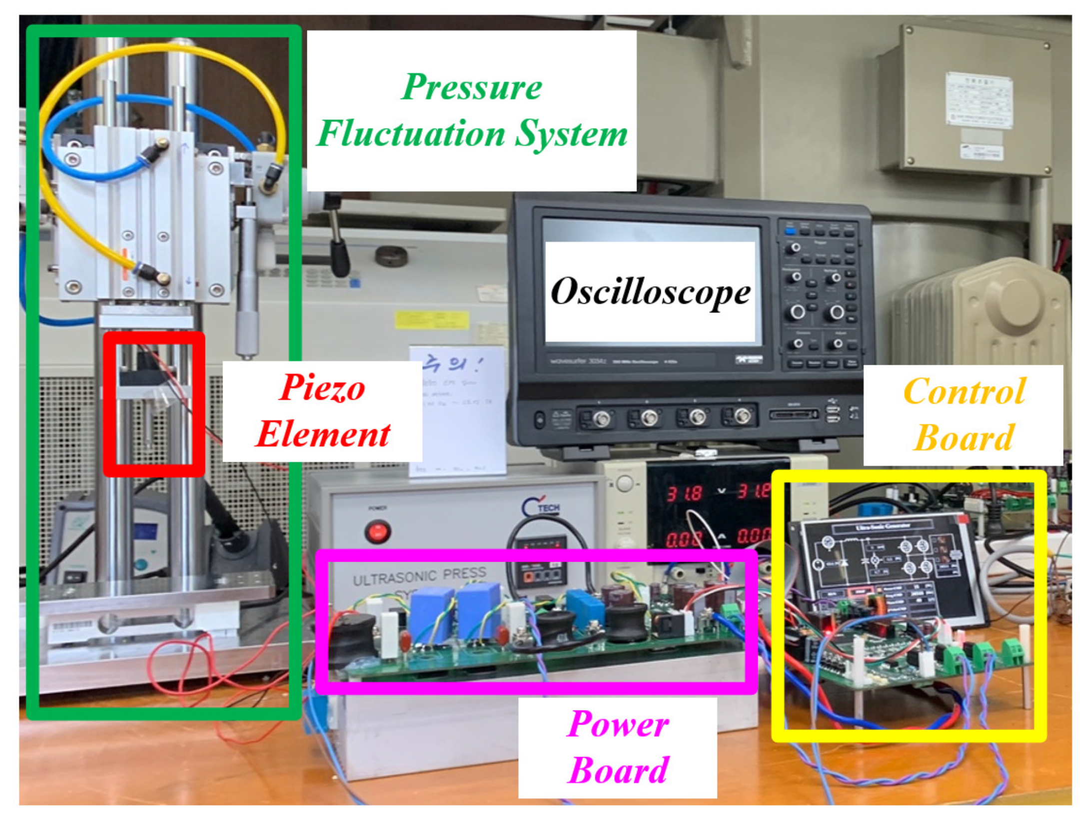
4. Experimental Results

This section presents the experimental results obtained by operating the ultrasonic system at the estimated mechanical resonant frequency of the piezo element using the LSTM model.

Figure 15 shows the experimental environment and configuration. The configuration consists of a control board, a power board, a piezo element, and a pressure press system for applying the user’s desired pressure to the piezo element. The press system for applying pressure to the piezo element is designed to detect pressure in real time using a strain gauge and to apply pressure in the vertical direction to the piezo element. Through this, conditions for always applying a constant pressure to the piezo element can be created, and the variation in the procedure can be minimized for analysis.

Figure 16 shows the actual system operation results on the relationship graph between the resonant frequency of the ultrasonic system and the mechanical resonant frequency of the piezo element. In the graph, the x-axis represents the entire system resonant frequency at the ultrasonic system output stage and the y-axis represents the mechanical resonant frequency of the piezo element. The red points within the graph indicate the mechanical resonant frequencies of the piezo element at different system resonant frequencies under various applied pressures, ranging from 0 g to 5000 g in 250 g increments. The waveform below corresponds to a pressure of 1000 g. The control algorithm is divided into three modes: Mode 1, the initial operation stage, applies PWM switching at the designed resonant frequency of the piezo element. Mode 2 detects the system resonant frequency using a frequency detection circuit and calculates the mechanical resonant frequency of the piezo element. Mode 3 operates at the calculated mechanical resonant frequency of the piezo element. The transitions between modes are confirmed using a trigger signal. The following presents the experimental waveforms at the input stage of the piezo element. The control algorithm’s three stages were verified during the experiment.

Figure 17 shows the initial 31.95 kHz PWM switching operation in Mode 1 and the operation transition to Mode 2, demonstrating the phase difference between the voltage and current of the piezo element in both modes.

Figure 18 shows the transition from Mode 2 to Mode 3. Near the end of the system resonant frequency detection in Mode 2, the voltage and current phases of the piezo element appear almost aligned, indicating the transient state rather than the actual mechanical resonant frequency.

Figure 19 illustrates the stable switching at the calculated frequency in Mode 3 based on the LSTM model’s estimated mechanical resonant frequency of the piezo element and the detected system resonant frequency of 31.221 kHz from Mode 2. Comparing the LSTM model’s estimated data in Figure 20, the mechanical resonant frequency of the piezo element was accurately estimated to be 30.618 kHz.

The above experimental results show that the method using the LSTM model is more efficient than the existing frequency tracking method (the method using PLL). PLL is basically well suited to linear systems, and the accuracy may decrease when the system has strong nonlinearity. On the other hand, LSTM can learn complex temporal dependencies, including nonlinearity, so it can better model the complex response of the piezo element. In addition, as shown in the analysis results in Chapter 2 of this study, a piezo element can have multiple resonance modes in addition to one mechanical resonance frequency. Since LSTM shows strength in simultaneously learning and predicting multiple modes, it is effective even in complex systems with multiple frequency modes. The mechanical resonance frequency estimation of a piezo element using the LSTM model can show superior performance in various aspects, such as complex nonlinear system processing, flexible adaptation to environmental changes, robustness to noise, and real-time processing capability, compared to the existing method. In addition, it can reduce hardware complexity and integrate the influence of various environmental variables to enable more accurate and stable frequency estimation. The LSTM model used in the experiment is the result of creating a model for six parameters (ultrasonic system resonance frequency ($f_{system}$), piezo element mechanical resonance frequency ($f_{piezo}$), piezo element parameter values $L_1$ and $C_1$, and $L_f$ and $C_f$ of the $LC$ filter). In other words, it is a limited experimental result in estimating the mechanical resonance frequency of the piezo element. The piezo element has various variables, such as mechanical quality factor Qm, loss factor Q, and piezoelectric coefficient. Therefore, there are limitations in this study, and it is a future task to study the discussion on the prediction and experimental verification of the LSTM model using various parameters of the piezo element. These experimental results validate the effectiveness of using the LSTM model to estimate the mechanical resonant frequency of the piezo element and deliver maximum power to it.

5. Conclusions

In this paper, we propose a method to estimate the optimal resonance frequency through regression analysis to maximize the mechanical output of the piezo element by measuring the frequency of the entire system combined with the input $LC$ filter and the piezo element. The validity of the proposed method was verified through MATLAB simulation and ultrasonic system experiments, and the following conclusions can be summarized.

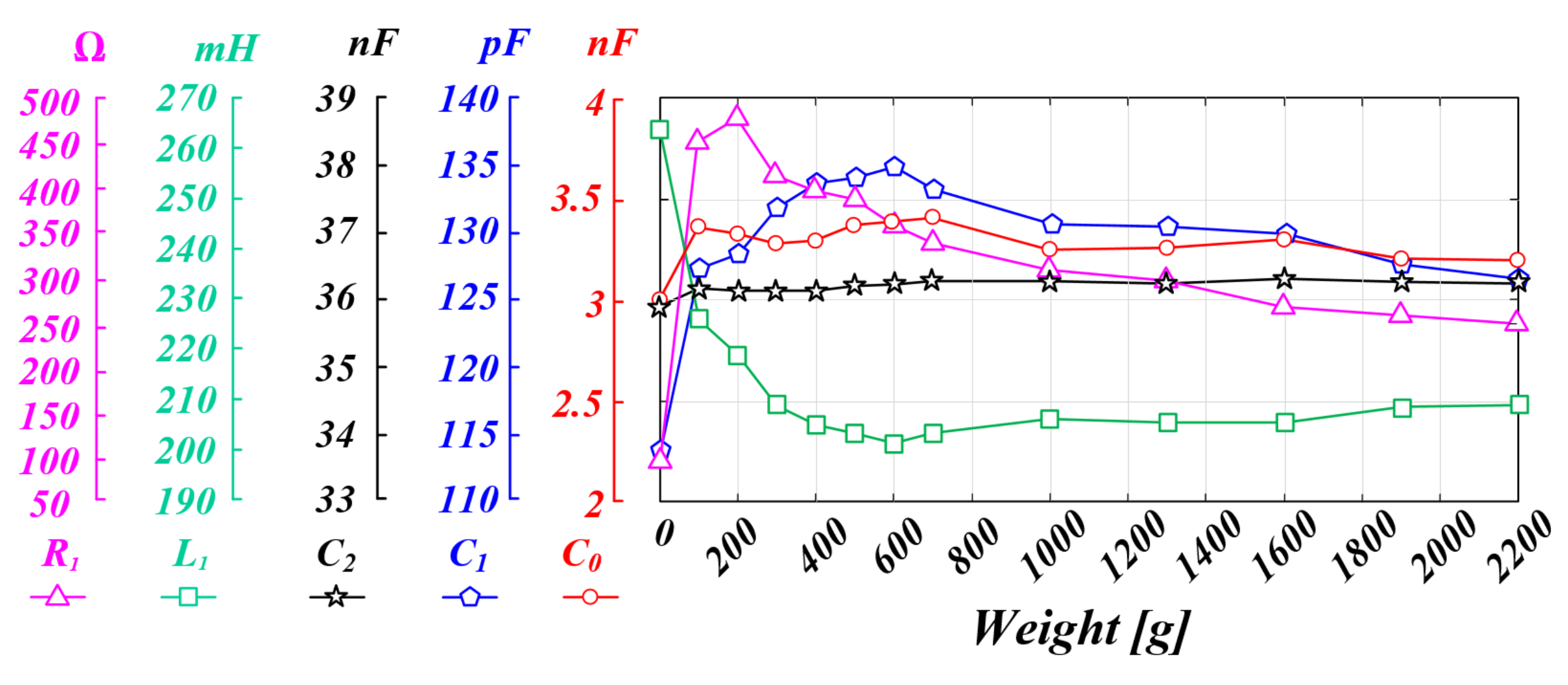
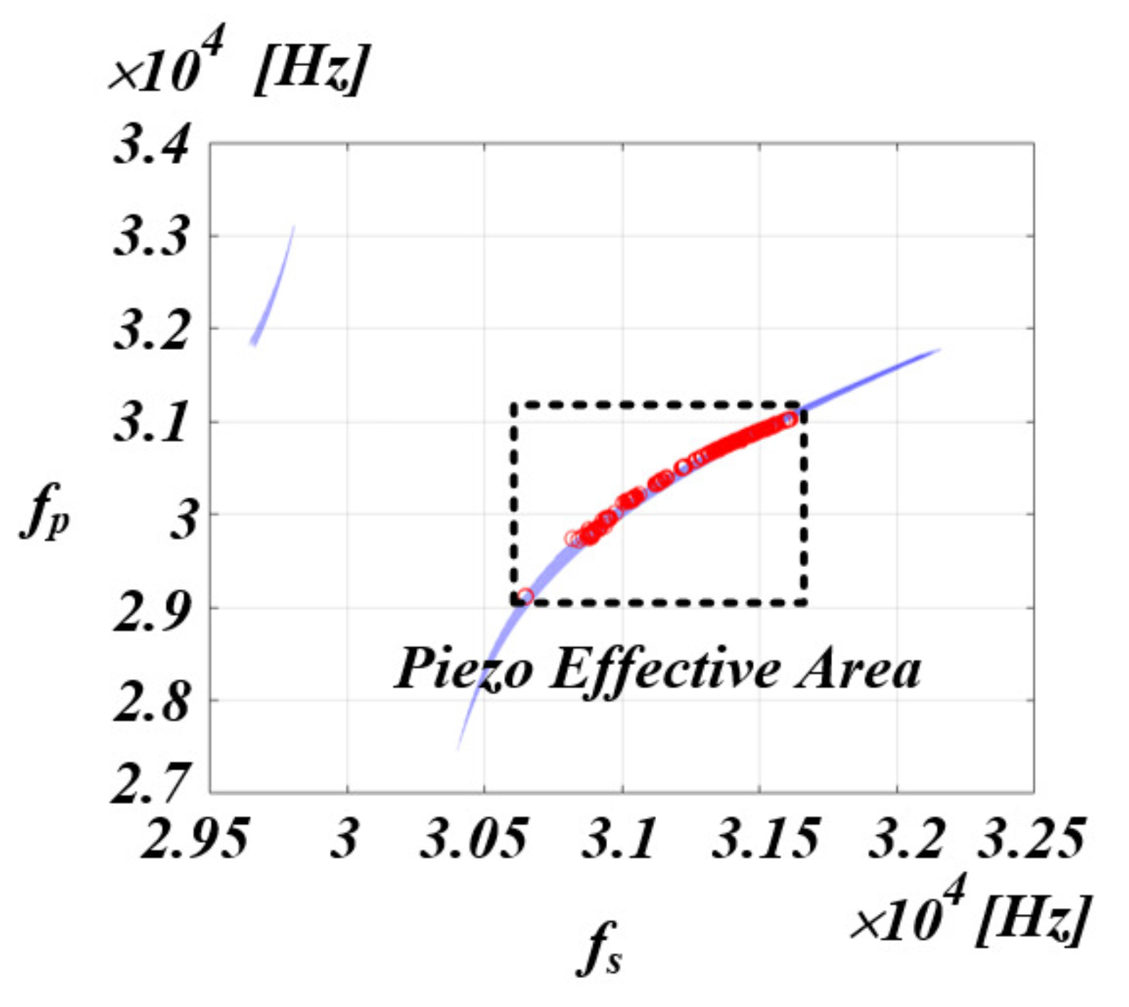
• The mechanical resonance frequency of the piezo element in the ultrasonic system shows nonlinear characteristics. Therefore, a system design that considers the characteristics of the piezo element is necessary. This includes the theory of selecting each parameter value in the $LC$ filter section and impedance matching to match the resonance frequency of the inverter output stage and the resonance frequency of the piezo element as similarly as possible in the ultrasonic system.
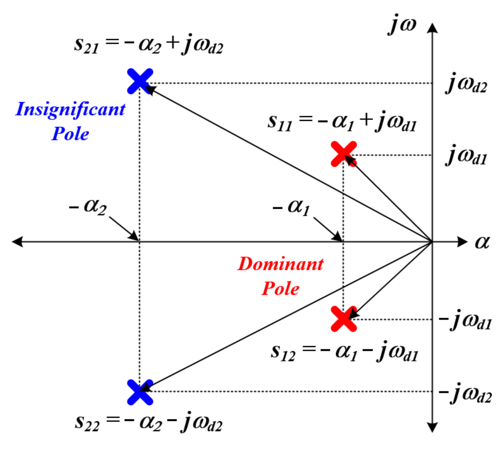
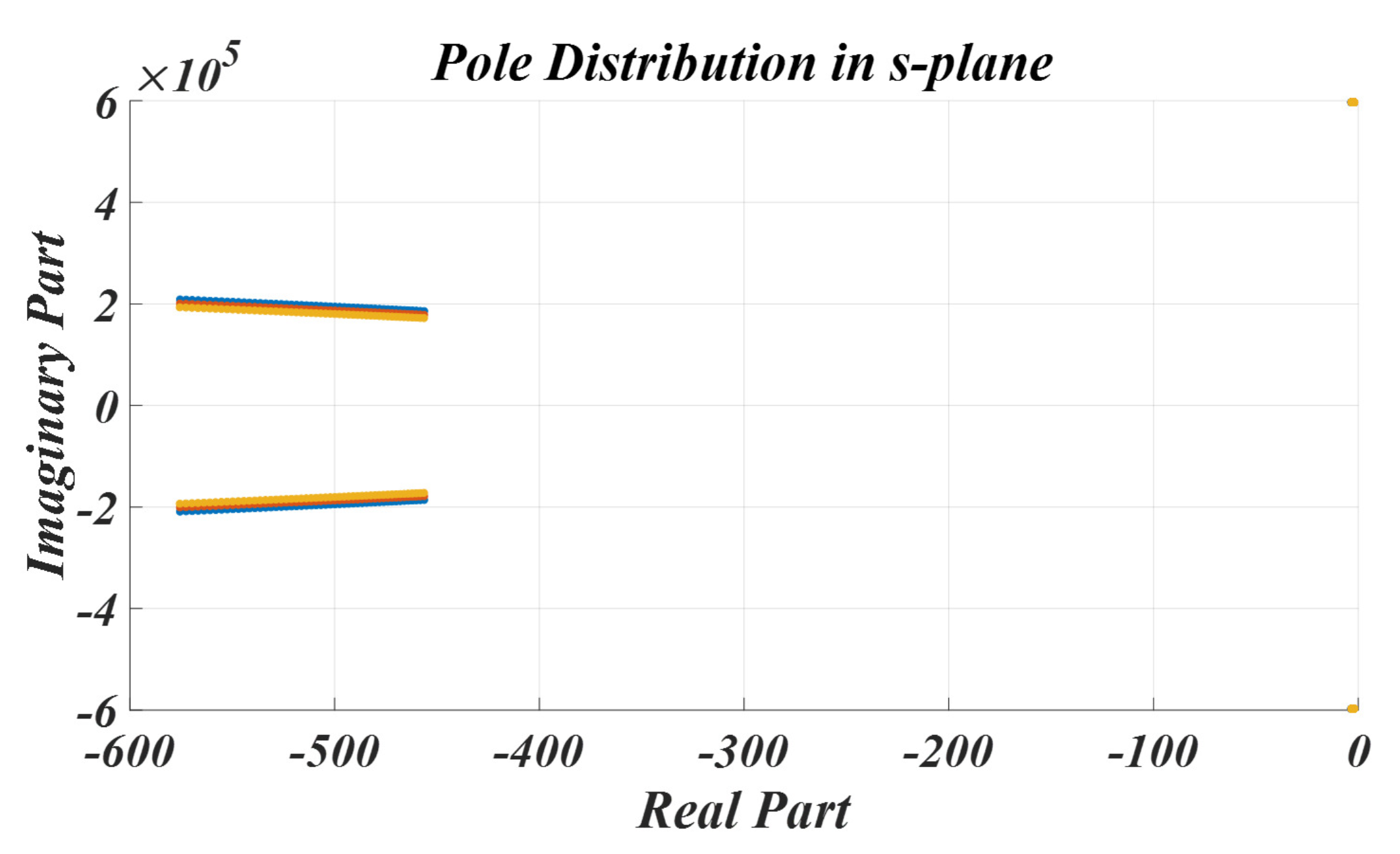
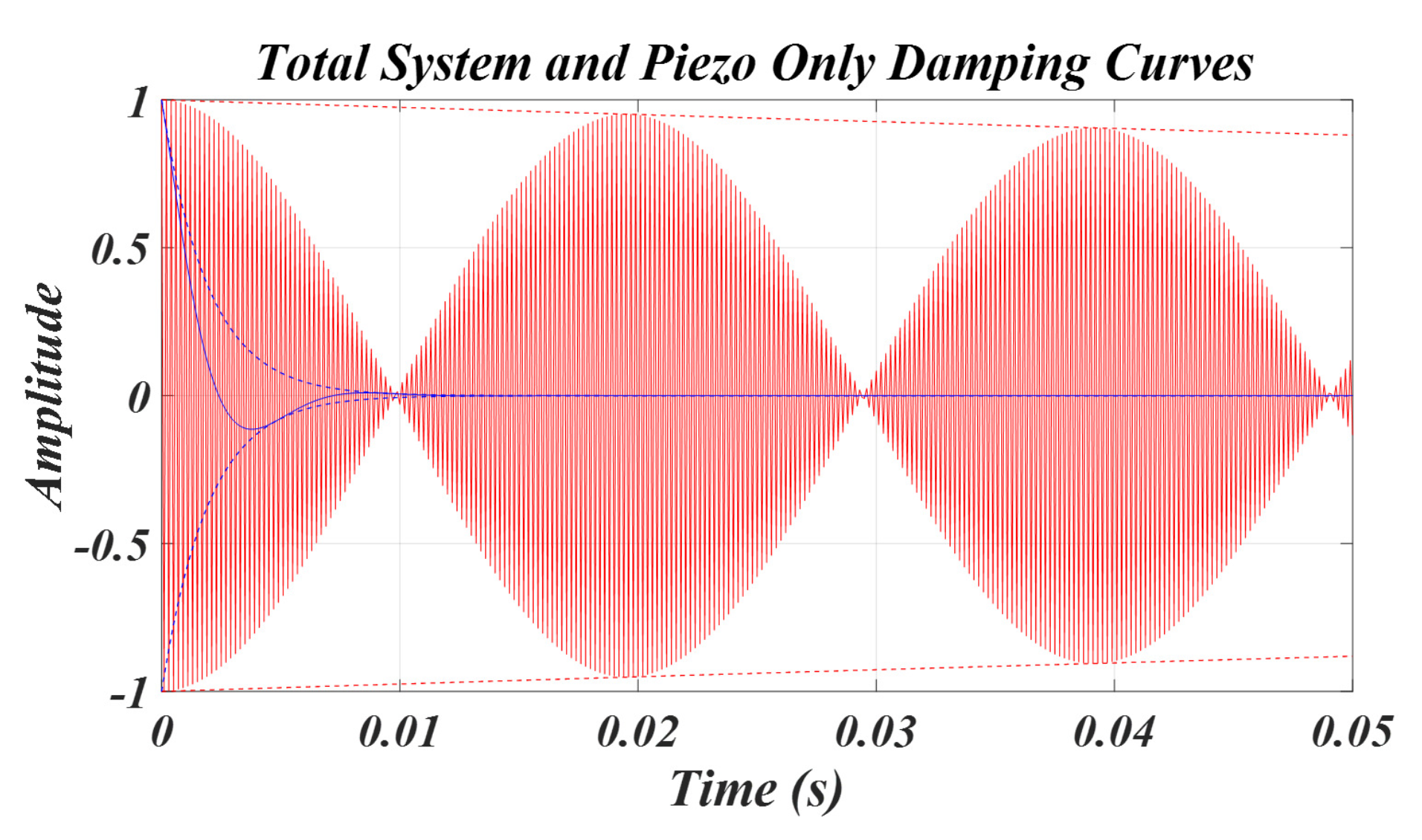
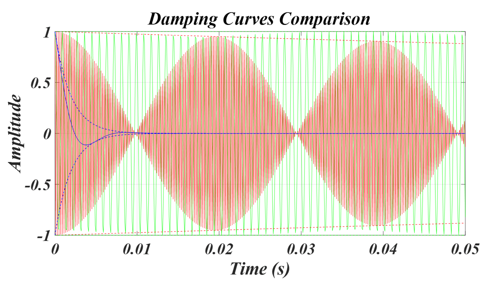
• In order to operate the system at the mechanical resonance frequency to transmit maximum power to the piezo element, the creation of an equivalent model of the piezo element and an analysis of the resonance characteristics were performed. In addition, the system was designed by analyzing the impedance of the series $R_1$$L_1$$C_1$ circuit that affects the mechanical output of the $LC$ filter and the piezo element. Through this, the relationship between the system resonance frequency and the mechanical resonance frequency of the piezo element was analyzed by calculating the characteristic equation, calculating the characteristic root, calculating the damping period, and calculating the vibration period.
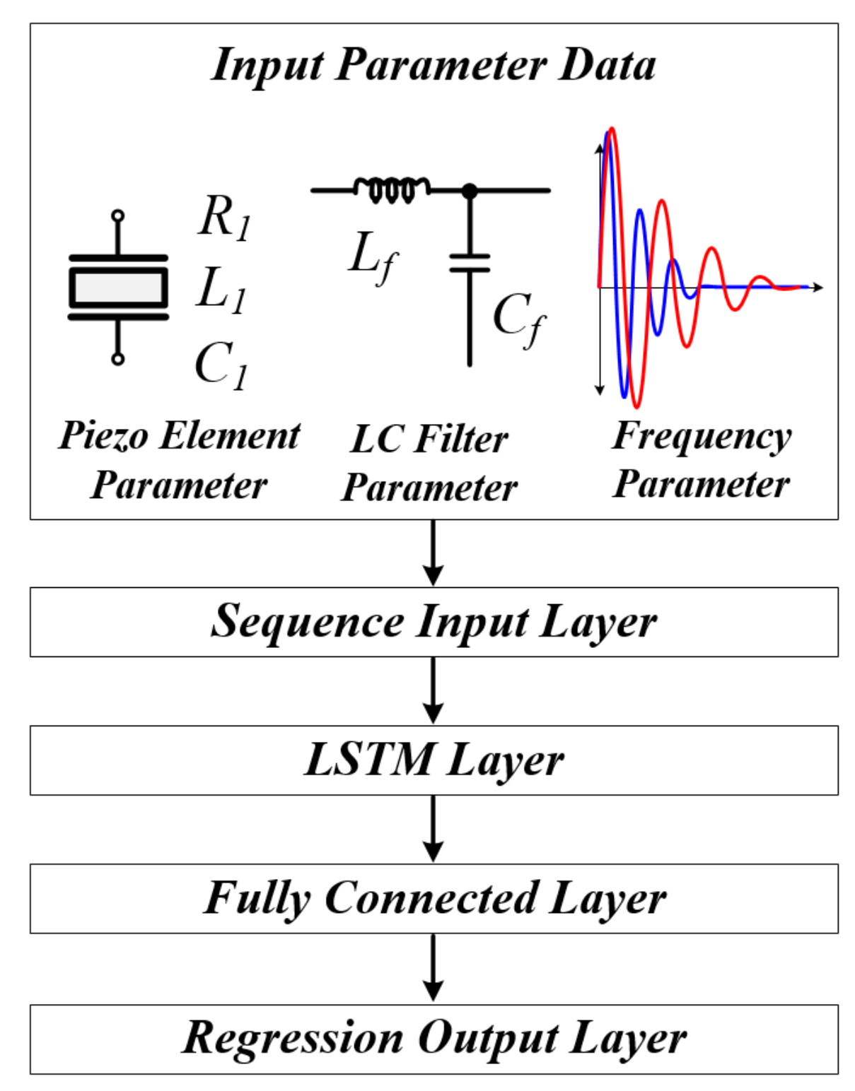
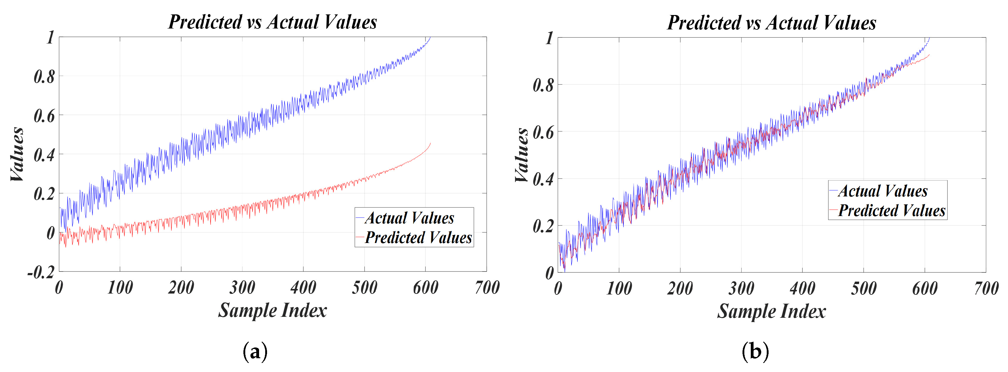
• The LSTM model was used to utilize the mechanical resonance frequency of the piezo element for efficient operation of the ultrasonic system. As a result, a method to estimate the characteristics of the entire mechanical resonance frequency range of the piezo element using the LSTM model was proposed. The relationship was verified through the analysis of the mechanical resonance frequency of the piezo element, the entire system resonance frequency of the ultrasonic system inverter output stage, and the parameter values $L_f$ and $C_f$ of the $LC$ filter, and the piezo mechanical resonance frequency was estimated through this. In addition, the LSTM model showed more accurate mechanical resonance frequency estimation results than the nonlinear regression model in the piezo element with nonlinear characteristics.
• Since the LSTM model can learn complex temporal dependencies, including nonlinearity, it can better model the complex response of the piezoelectric element. Since the LSTM model shows strength in simultaneously learning and predicting multiple modes, it is effective even in complex systems with multiple frequency modes. The estimation of the mechanical resonance frequency of a piezoelectric element using the LSTM model can show superior performance in processing complex nonlinear systems compared to existing methods. In addition, it can enable more accurate and stable frequency estimation.

From this study, it can be seen that using the LSTM model is effective in estimating the mechanical resonance frequency of the piezoelectric element, and it is thought that it will be effective to analyze other systems that require resonance frequency estimation using the LSTM model in the future.

References

1. Kentish, S.; Feng, H. Applications of power ultrasound in food processing. Annu. Rev. Food Sci. Technol. 2014, 5, 263–284. [Google Scholar] [CrossRef]
2. Luong, V.D.; Duong, P.T.M.; Nguyen, T.B.N.; Ngo, N.K.; Nguyen, T.H. Dynamic response of high-power ultrasonic system based on finite element modeling of piezoelectric. J. Appl. Eng. Sci. 2023, 21, 859–871. [Google Scholar] [CrossRef]
3. Wellendorf, A.; von Damnitz, L.; Nuri, A.W.; Anders, D.; Trampnau, S. Determination of the temperature-dependent resonance behavior of ultrasonic transducers using the finite-element method. J. Vib. Eng. Technol. 2024, 12, 1277–1290. [Google Scholar] [CrossRef]
4. Chen, J.; Li, P.; Song, G.; Ren, Z. Piezo-based wireless sensor network for early-age concrete strength monitoring. Optik 2016, 127, 2983–2987. [Google Scholar] [CrossRef]
5. Tao, Y.; Hwachun, L.; Dongheon, L.; Sunggun, S.; Dongok, K.; Sungjun, P. Design of LC Resonant Inverter for Ultrasonic Metal Welding System. In Proceedings of the 2008 International Conference on Smart Manufacturing Application, Goyangi, Republic of Korea, 9–11 April 2008; pp. 543–548. [Google Scholar]
6. Fernández-Afonso, Y.; García-Zaldívar, O.; Calderón-Piñar, F. Equivalent circuit for the characterization of the resonance mode in piezoelectric systems. J. Adv. Dielectr. 2015, 5, 1550032. [Google Scholar] [CrossRef]
7. Lin, S.; Xu, J. Effect of the matching circuit on the electromechanical characteristics of sandwiched piezoelectric transducers. Sensors 2017, 17, 329. [Google Scholar] [CrossRef] [PubMed]
8. Wang, T.; Dupont, J.; Tang, J. On integration of vibration suppression and energy harvesting through piezoelectric shunting with negative capacitance. IEEE/ASME Trans. Mechatron. 2023, 28, 2621–2632. [Google Scholar] [CrossRef]
9. Yu, H.; Zhou, J.; Deng, L.; Wen, Z. A vibration-based MEMS piezoelectric energy harvester and power conditioning circuit. Sensors 2014, 14, 3323–3341. [Google Scholar] [CrossRef]
10. Malikan, M.; Eremeyev, V.A. On the dynamics of a visco–piezo–flexoelectric nanobeam. Symmetry 2020, 12, 643. [Google Scholar] [CrossRef]
11. Jiang, W.W.; Gao, X.W. Analysis of thermo-electro-mechanical dynamic behavior of piezoelectric structures based on zonal Galerkin free element method. Eur. J.-Mech.-A/Solids 2023, 99, 104939. [Google Scholar] [CrossRef]
12. Yang, C.; Sun, H.; Liu, S.; Qiu, L.; Fang, Z.; Zheng, Y. A Broadband Resonant Noise Matching Technique for Piezoelectric Ultrasound Transducers. IEEE Sensors J. 2019, 20, 4290–4299. [Google Scholar] [CrossRef]
13. Rathod, V.T. A review of electric impedance matching techniques for piezoelectric sensors, actuators and transducers. Electronics 2019, 8, 169. [Google Scholar] [CrossRef]
14. Wang, J.D.; Jiang, J.J.; Duan, F.J.; Cheng, S.Y.; Peng, C.X.; Liu, W.; Qu, X.H. A high-tolerance matching method against load fluctuation for ultrasonic transducers. IEEE Trans. Power Electron. 2019, 35, 1147–1155. [Google Scholar] [CrossRef]
15. Ju, B.; Fang, L.; Wang, Q.; Xu, J.; Li, G.; Liu, Y. General rules for the inductive characteristics of a piezoelectric structure and its integration with piezoelectric transformer for capacitive compensation. Smart Mater. Struct. 2021, 30, 045018. [Google Scholar] [CrossRef]
16. Pan, Z.; Ren, D.; Spiazzi, G.; Wei, S.; Yang, J.; Nie, B.L.; Du, P. An equivalent modeling method of passive components with multi-resonant frequency. Int. J. Circuit Theory Appl. 2023, 51, 2689–2704. [Google Scholar] [CrossRef]
17. Kumar, P.; Leonardi, N. Exploring mega-nourishment interventions using Long Short-Term Memory (LSTM) models and the sand engine surface MATLAB framework. Geophys. Res. Lett. 2024, 51, e2023GL106042. [Google Scholar] [CrossRef]
18. Sabareesh, S.; Aravind, K.; Chowdary, K.B.; Syama, S.; VS, K.D. LSTM based 24 h ahead forecasting of solar PV system for standalone household system. Procedia Comput. Sci. 2023, 218, 1304–1313. [Google Scholar] [CrossRef]
19. Parida, L.; Moharana, S.; Ferreira, V.M.; Giri, S.K.; Ascensão, G. A novel CNN-LSTM hybrid model for prediction of electro-mechanical impedance signal based bond strength monitoring. Sensors 2022, 22, 9920. [Google Scholar] [CrossRef]
20. Yang, R.; Singh, S.K.; Tavakkoli, M.; Amiri, N.; Yang, Y.; Karami, M.A.; Rai, R. CNN-LSTM deep learning architecture for computer vision-based modal frequency detection. Mech. Syst. Signal Process. 2020, 144, 106885. [Google Scholar] [CrossRef]
21. Hoseyni, S.M.; Aghakhani, A.; Basdogan, I. Experimental admittance-based system identification for equivalent circuit modeling of piezoelectric energy harvesters on a plate. Mech. Syst. Signal Process. 2024, 208, 111016. [Google Scholar] [CrossRef]
22. Wang, J.; Xiong, C.; Huang, J.; Peng, J.; Zhang, J.; Zhao, P. Waveform design method for piezoelectric print-head based on iterative learning and equivalent circuit model. Micromachines 2023, 14, 768. [Google Scholar] [CrossRef]
23. Duan, B.; Wu, K.; Chen, X.; Ni, J.; Ma, X.; Meng, W.; Lam, K.h.; Yu, P. Bioinspired PVDF piezoelectric generator for harvesting multi-frequency sound energy. Adv. Electron. Mater. 2023, 9, 2300348. [Google Scholar] [CrossRef]
24. Zhang, Y.; Yang, T.; Du, H.; Zhou, S. Wideband vibration isolation and energy harvesting based on a coupled piezoelectric-electromagnetic structure. Mech. Syst. Signal Process. 2023, 184, 109689. [Google Scholar] [CrossRef]
25. Bonnin, M.; Song, K. Frequency domain analysis of a piezoelectric energy harvester with impedance matching network. Energy Harvest. Syst. 2023, 10, 135–144. [Google Scholar] [CrossRef]
26. Zhang, K.; Gao, G.; Zhao, C.; Wang, Y.; Wang, Y.; Li, J. Review of the design of power ultrasonic generator for piezoelectric transducer. Ultrason. Sonochem. 2023, 96, 106438. [Google Scholar] [CrossRef]
27. Taşlıyol, M.; Öncü, S.; Turan, M.E. An implementation of class D inverter for ultrasonic transducer mixed powder mixture. Ultrason. Sonochem. 2024, 104, 106838. [Google Scholar] [CrossRef]
28. Asemi, Z.; Beiranvand, R. Using a High Frequency LC Resonant Inverter for Ultrasonic Cleaning Applications. In Proceedings of the 2023 14th Power Electronics, Drive Systems, and Technologies Conference (PEDSTC), Babol, Iran, 31 January–2 February 2023; pp. 1–6. [Google Scholar]
29. Cai, Y.; He, Y.; Zhang, H.; Zhou, H.; Liu, J. Integrated design of filter and controller parameters for low-switching-frequency grid-connected inverter based on harmonic state-space model. IEEE Trans. Power Electron. 2023, 38, 6455–6473. [Google Scholar] [CrossRef]
30. Moon, J.; Park, S.; Lim, S. A novel high-speed resonant frequency tracking method using transient characteristics in a piezoelectric transducer. Sensors 2022, 22, 6378. [Google Scholar] [CrossRef] [PubMed]
31. Ruderman, M. Time-delay based output feedback control of fourth-order oscillatory systems. Mechatronics 2023, 94, 103015. [Google Scholar] [CrossRef]
32. Cao, Q. Dynamic surface sliding mode control of chaos in the fourth-order power system. Chaos Solitons Fractals 2023, 170, 113420. [Google Scholar] [CrossRef]
33. Dincel, E.; Söylemez, M.T. Limitations on Dominant Pole Pair Selection with Continuous PI and PID Controllers. In Proceedings of the 2016 International Conference on Control, Decision and Information Technologies (CoDIT), Saint Julian’s, Malta, 6–8 April 2016; pp. 741–745. [Google Scholar]
34. Dai, Y.; Li, D.; Wang, D. Review on the nonlinear modeling of hysteresis in piezoelectric ceramic actuators. Actuators 2023, 12, 442. [Google Scholar] [CrossRef]
35. Alrbai, M.; Alahmer, H.; Alahmer, A.; Al-Rbaihat, R.; Aldalow, A.; Al-Dahidi, S.; Hayajneh, H. Retrofitting conventional chilled-water system to a solar-assisted absorption cooling system: Modeling, polynomial regression, and grasshopper optimization. J. Energy Storage 2023, 65, 107276. [Google Scholar] [CrossRef]
36. Zuo, Y.; Zuo, H. Least sum of squares of trimmed residuals regression. Electron. J. Stat. 2023, 17, 2416–2446. [Google Scholar] [CrossRef]
37. Wang, Z.; Cai, Y.; Liu, D.; Qiu, F.; Sun, F.; Zhou, Y. Intelligent classification of coal structure using multinomial logistic regression, random forest and fully connected neural network with multisource geophysical logging data. Int. J. Coal Geol. 2023, 268, 104208. [Google Scholar] [CrossRef]
38. Aigrain, S.; Foreman-Mackey, D. Gaussian process regression for astronomical time series. Annu. Rev. Astron. Astrophys. 2023, 61, 329–371. [Google Scholar] [CrossRef]
Figure 1. Piezo element equivalent circuit model.
Applsci 14 07833 g001
Figure 2. Parameter variation characteristics of the piezo element with pressure changes.
Applsci 14 07833 g002
Figure 3. Equivalent circuit of the ultrasonic entire system.
Applsci 14 07833 g003
Figure 4. Equivalent circuit of the ultrasonic entire system impedance separation 1.
Applsci 14 07833 g004
Figure 5. Equivalent circuit of the ultrasonic entire system impedance separation 2.
Applsci 14 07833 g005
Figure 6. Fourth-order system in the s-plane.
Applsci 14 07833 g006
Figure 7. Response characteristics of the fourth-order system.
Applsci 14 07833 g007
Figure 8. S-plane graph of pressure variations in piezo elements.
Applsci 14 07833 g008
Figure 9. Dampingcharacteristics graph 1 of ultrasonic system and piezo elements.
Applsci 14 07833 g009
Figure 10. Damping characteristics graph 2 of ultrasonic system and piezo elements.
Applsci 14 07833 g010
Figure 11. Graph of the relationship between ultrasonic system resonant frequency and mechanical resonant frequency of piezo elements.
Applsci 14 07833 g011
Figure 12. LSTM model used in the experiment.
Applsci 14 07833 g012
Figure 13. Estimation of mechanical resonant frequency of piezo elements using nonlinear regression model and LSTM model 1.
Applsci 14 07833 g013
Figure 14. Estimation of mechanical resonant frequency of piezo elements using nonlinear regression model and LSTM model 2.
Applsci 14 07833 g014
Figure 15. Ultrasonic system experimental environment and configuration.
Applsci 14 07833 g015
Figure 16. Actual system operation results in the resonant frequency relationship graph.
Applsci 14 07833 g016
Figure 17. Operation waveform 1 (piezo element voltage, current waveform).
Applsci 14 07833 g017
Figure 18. Operation waveform 2 (piezo element voltage, current waveform).
Applsci 14 07833 g018
Figure 19. Operation waveform 3 (piezo element voltage, current waveform).
Applsci 14 07833 g019
Figure 20. Data for estimation of mechanical resonant frequency of piezo elements.
Applsci 14 07833 g020