Abstract
Many systems in the manufacturing industry have spatial distribution characteristics, which correlate with both time and space. Such systems are known as distributed parameter systems (DPSs). Due to the spatiotemporal coupling characteristics, the modeling of such systems is quite complex. The paper presents a new approach for three-dimensional fuzzy modeling using Simultaneous Perturbation Stochastic Approximation (SPSA) for nonlinear DPSs. The Affinity Propagation clustering approach is utilized to determine the optimal number of fuzzy rules and construct a collection of preceding components for three-dimensional fuzzy models. Fourier space base functions are used in the resulting components of three-dimensional fuzzy models, and their parameters are learned by the SPSA algorithm. The proposed three-dimensional fuzzy modeling technique was utilized on a conventional DPS within the semiconductor manufacturing industry, with the simulation experiments confirming its efficacy.
1. Introduction
The spatial distribution characteristics are widely present in many manufacturing industries such as petroleum, chemical, steelmaking, and rolling. The dynamic characteristics of the system change with time and space, and this type of system is called a distributed parameter system (DPS) [1]. The dynamic characteristics of DPSs are usually described by partial differential equations and integral equations. Traditionally, the spatial distribution characteristics of such systems are often ignored, and the inherent DPSs are approximated as lumped parameter systems (LPS), and then are modeled and controlled using the mature lumped parameter methods. With the development in the times, people’s requirements for product quality are gradually increasing. With the advancement of sensors, actuators, and computing technology, the modeling, control, and optimization techniques of DPSs have received increasing attention in the fields of science and engineering. For practical use in areas like the optimization, control design, analyzing, and numerical simulations of DPSs [2], it is necessary to use an appropriate mathematical model to describe its dynamic characteristics. Therefore, the modeling of DPSs has become a very important research field.
The modeling methods for DPSs can usually be divided into mechanism modeling with known partial differential equations and grey-box/black-box modeling with unknown partial differential equations. Mechanism modeling is the process of obtaining partial differential equations for DPSs from the point of view of physical or chemical reaction knowledge of the system, such as thermal energy balance, material balance, or momentum balance relationships. Considering the complexity of calculations and the restricted quantity of sensors and actuators, modeling such systems further requires the use of spectral methods [1], finite elements [3], finite difference techniques, etc., to simplify the essentially infinite dimensional system into a finite dimensional system [4]. Nonetheless, in real-world scenarios, it will be challenging to obtain accurate mathematical descriptions of the system through the mechanism modeling method due to incomplete knowledge of physical and chemical processes. The second modeling method is based on data, including grey-box modeling and black-box modeling [5]. The model expressed by partial differential equations of the system is established through prior knowledge, and the unknown parameters of the model are obtained by identification from the input/output data of the system. This method is called grey-box modeling. Directly identifying the structure and parameters of a system from input/output data is called black-box modeling. In practical applications, black-box modeling has a wider range of applications. How to extract the relationship between system inputs/outputs with spatial distribution characteristics from data is currently a challenge in modeling research.
In recent decades, researchers have conducted continuous research on black-box modeling of DPS. A few studies first discretized the PDE system in space and time, and then proposed the physical informed spark learning method to optimize the model parameters [6]. However, there is a linear relationship between the dimension of the system and the product of space–time discrete quantity, resulting in many model parameters. Most methods decompose variables into a series of spatial functions and temporal coefficients [7] and then reconstruct the system. Traditional methods usually preset spatial functions, such as Jacobian polynomials, spline functions, etc., and prior knowledge also dictates the quantity of spatial functions. The time coefficients are estimated using traditional modeling methods for LPS. In the past 20 years, spatial functions have been estimated using the Karhunen–Loève (KL) decomposition method [8,9]. The time coefficient is still estimated using traditional modeling methods for LPS. In practical applications, essentially infinite dimensional systems require model simplification to obtain lower-order ordinary differential equations. However, model simplification can lead to unmodeled dynamics and unknown nonlinearity [10].
Intelligent methods like neural networks, extreme learning machines, and fuzzy systems have been incorporated into DPS modeling as well. References [9,11,12,13] combined neural networks with space–time separation methods and achieved good experimental results on parabolic DPS modeling problems. Wang et al. [11] used a nonlinear PCA method to obtain space base functions. After space–time separation and dimension reduction, a neural network was used to identify the time coefficients. Zhang et al. [12] used the PCA algorithm to obtain space base functions. After space–time separation and dimension reduction, the time model was decomposed into linear and nonlinear parts. The ARX model was used to model the linear part, and the RBF neural network was employed to model the nonlinear part. Fan et al. [9] used the KL decomposition method to obtain space base functions. After space–time separation and dimension reduction, a mixed time series model of long short-term memory network and multi-layer perceptron was used to model the time coefficients. Wang et al. [13] employed the incremental KL method to estimate the spatial basis function, and utilized the RBF neural network to establish the time model. After linearization, the spatiotemporal model was used for the model predictive control of an oven. Chen et al. [14] mainly solved the problem of using many sensors in KL decomposition-based modeling, and proposed a two-step modeling method. Firstly, the KL method was used to obtain the spatial basis function by using many sensors offline; then the sensors were reduced, the spatial mapping filtering method was used to obtain the output information without sensor points, and the incremental KL method was used to update the spatial basis function; finally, the extreme learning machine was used to learn time model. Unlike the KL decomposition method, Jin et al. [15] first used the locally linear embedding technique to reduce the dimension and obtain the time coefficient; then they used extreme learning machine to establish the time model, and finally used the kernel-based extreme learning machine to reconstruct the spatiotemporal coupling output. However, the aforementioned modeling methods still require dimension reduction.
Three-dimensional fuzzy modeling [10,16] is a new type of DPS modeling method that has developed in the past five years. In three-dimensional fuzzy model, the functions of space–time separation and space–time reconstruction are naturally integrated into three-dimensional fuzzy rules. In each three-dimensional fuzzy rule, space–time separation is naturally achieved, where the preceding component is computed as the time factor, and the resulting component is regarded as the space base function. In the combination operation of multiple excited three-dimensional fuzzy rules, space–time reconstruction is naturally achieved. Compared with traditional modeling methods of distributed parameter systems, the three-dimensional fuzzy modeling method has two advantages: it does not rely on model dimension reduction and has language interpretability.
At present, the three-dimensional fuzzy model has been applied in the modeling of DPS such as rapid thermal processing and chemical reactors. Zhang et al. [10] introduced a three-dimensional fuzzy modeling approach utilizing clustering and support vector regression, where the nearest neighbor clustering (NNC) method and similarity analysis technique were employed for mining and condensing the initial preceding components in the three-dimensional fuzzy rules, and support vector regression machines were employed to acquire knowledge about the space base functions of the resulting components in the three-dimensional fuzzy rules. However, the clustering results of the NNC algorithm are influenced by the initial representative point selection, and the structural simplification process is very cumbersome. Zhang et al. [16] proposed a method for three-dimensional fuzzy modeling that utilizes KL decomposition to derive space base functions for the resulting sets of the three-dimensional fuzzy rule. The resulting sets consist of a restricted amount of space base functions with higher weights. This method pertains to the scope of dimension reduction and results in dynamic characteristics that have not been modeled.
Based on the above discussion, this paper introduces an innovative three-dimensional fuzzy modeling method for DPS. Utilizing the Affinity Propagation (AP) clustering algorithm, the preceding components of the fuzzy rule are derived within the three-dimensional fuzzy modeling framework. By considering every data point as a potential class representative point, the AP algorithm circumvents the issue of clustering outcomes being constrained by the choice of initial class representative points. Unlike existing methods such as KL decomposition or support vector regression to learn space base functions, this paper sets the Fourier space base function as the resulting component of three-dimensional fuzzy rules. The construction of Fourier space base functions is simple and can better approximate the actual spatial distribution characteristics. Furthermore, the parameters of the Fourier space base function are fine-tuned using the simultaneous perturbation stochastic approximation (SPSA) algorithm.
The key innovations of this study are outlined below:
- (1)
- The AP clustering approach is utilized to determine the most suitable quantity of fuzzy rules and construct preceding sets for the three-dimensional fuzzy model.
- (2)
- The Fourier space base functions are initially introduced as the resulting sets of the three-dimensional fuzzy model.
- (3)
- The SPSA technique is employed to dynamically update the coefficients of Fourier space base functions for the three-dimensional fuzzy model.
2. Problem Description
2.1. Mathematical Description of Distributed Parameter Systems and Its Characteristics
Numerous processes, like the industrial chemical reaction [1], semiconductor production [17], transmission in cure or reflow processes [18] and Lithium-ion Battery Thermal Process [19,20], are spatially distributed in practice. They can be depicted using the subsequent mathematical formula:
where represents the output; is a nonlinear function; is the linear space differential operator, which includes first- or second-order spatial derivatives (), and is dense in Hilbert space; is a constant vector; is manipulating the input vector (i.e., multiple control sources); and is a known smooth function about f, which describes the distribution of Q in the spatial domain .
Usually, boundary and initial conditions also restrict the system depicted in Equation (1). As an illustration, at t = 1, the boundary and initial conditions can be depicted in the following equations:
where is dependent on and ; is dependent on and ; and is a known function.
This type of system has spatiotemporal coupling characteristics and is an infinite dimensional system. can be spatiotemporally separated into an infinite weighted sum of space base functions and time coefficients as shown in Equation (4):
where is a space base function and is a time coefficient.
Practically, it is necessary to utilize a finite quantity of sensors positioned at ; therefore, . represents the output in space, where P is the number of sensors. The data-driven modeling challenge for the DPS as outlined in Equations (1)–(3), entails the task of determining a spatiotemporal coupled model using the input and the output , where K is the time length. Essentially, systems with an infinite number of dimensions will be converted into systems with a finite number of dimensions. When the mechanism model described in Equations (1)–(3) is unknown, utilizing the KL decomposition technique, the system’s space base function can be derived from the gathered data set . Then, can be approximately depicted as Equation (5):
The time coefficients in Equation (5) can be identified using traditional methods.
However, the modeling approach of DPS using KL decomposition unavoidably results in neglected dynamic features and uncertainties in the identified model due to the decrease in dimensions.
2.2. Three-Dimensional Fuzzy Modeling
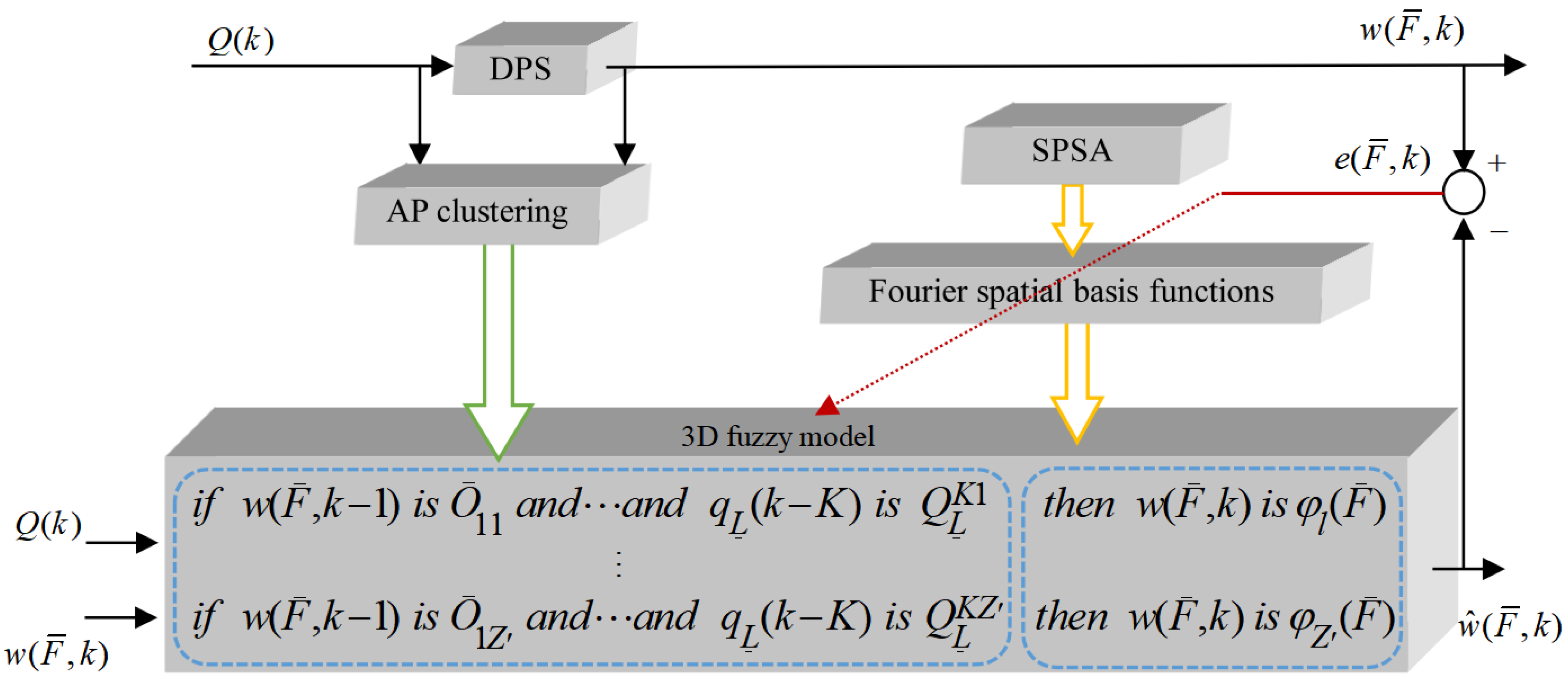
The three-dimensional fuzzy system [21] was first established in 2007 and has been used in the domain of DPS control [22]. Recently, there has been effective development in the three-dimensional fuzzy system for modeling DPS. The relevant theory of the three-dimensional fuzzy system and black-box modeling theory were combined to form a three-dimensional fuzzy modeling framework as shown in Figure 1 [10]. Unlike traditional modeling methods, the three-dimensional fuzzy modeling method can model a DPS without reduction in the dimension.
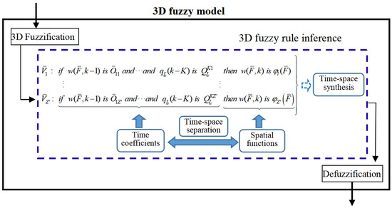
Figure 1.
Framework of three-dimensional fuzzy model (three-dimensional abbreviated as 3D).
Assume that K and J represent the order of the input variable and output variable , respectively. Input variables of three-dimensional fuzzy system are and . The three-dimensional fuzzy rule is given as shown in Equation (6):
where is a three-dimensional fuzzy set, is a conventional fuzzy set, , and indicates the count of fuzzy rules.
For any three-dimensional fuzzy rule , its preceding set ‘’ corresponds to the time coefficient . The resulting set ‘’ corresponds to the space base function , and space–time separation is ingeniously achieved through three-dimensional fuzzy rules. If three-dimensional fuzzy rules are excited, the time coefficients and space base functions of three-dimensional fuzzy rules will naturally realize space–time reconstruction. The final result is .
The three-dimensional fuzzy modeling framework can be divided into three parts:
- (1)
- Acquire the preceding set of fuzzy rules in order to derive temporal coefficients.
- (2)
- Acquire knowledge about the space base functions of the resulting set.
- (3)
- Obtain the predicted output through space–time reconstruction.
The study will explore an innovative approach to three-dimensional fuzzy modeling within this specific framework.
3. SPSA Learning-Based Three-Dimensional Fuzzy Modeling
3.1. Modeling Methodology
As for an unknown DPS system, space base functions are frequently calculated by the KL decomposition technique. However, implementing the KL decomposition technique is bound to result in the simplification of models. The three-dimensional fuzzy model has the innate ability to amalgamate space–time separation and space–time reconstruction into three-dimensional fuzzy rules and thereafter avoids the model reduction.
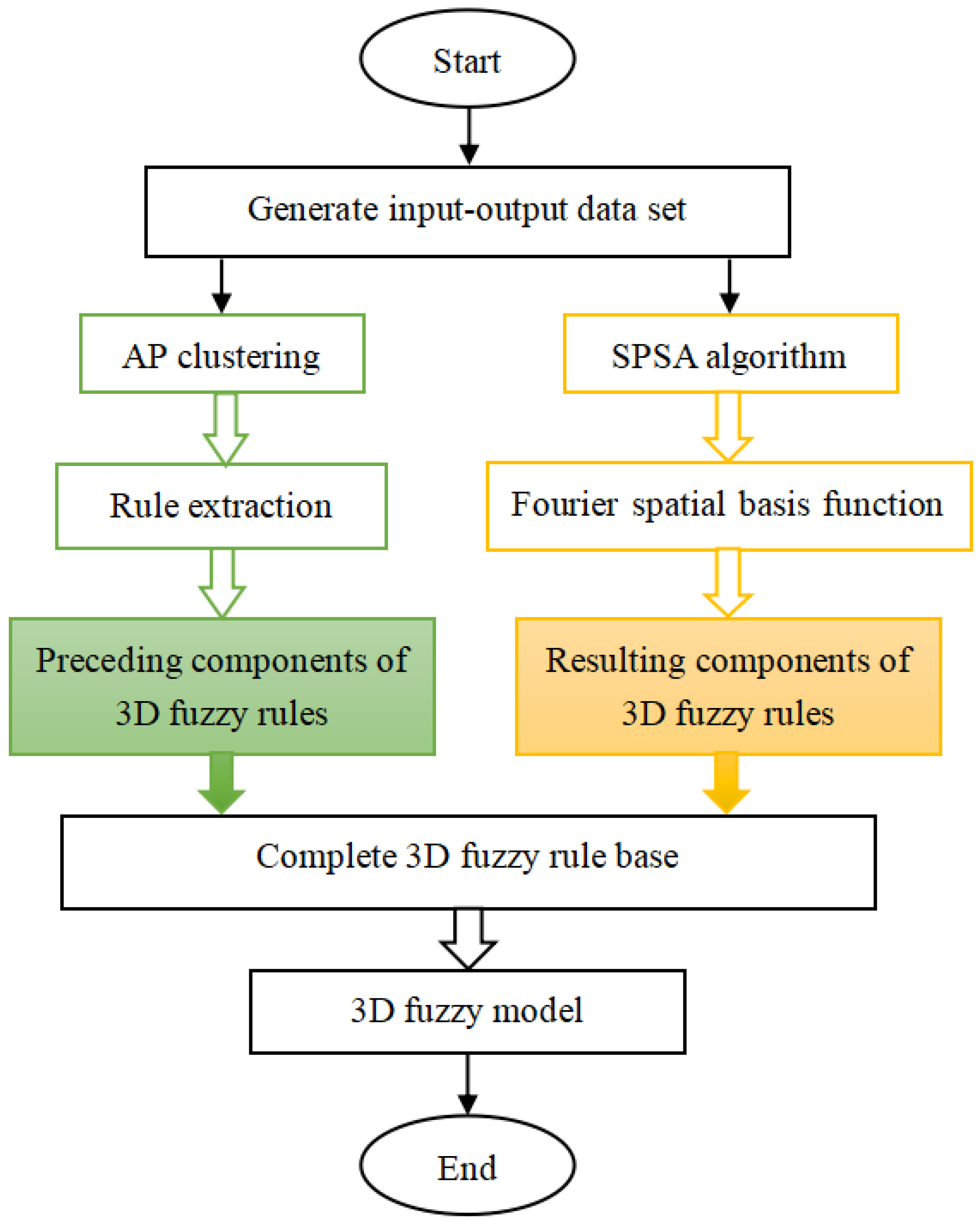
In this study, a novel SPSA learning-based three-dimensional fuzzy model methodology is proposed, the scheme of which is shown in Figure 2.
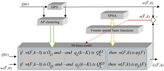
Figure 2.
Scheme of SPSA learning-based three-dimensional fuzzy modeling.
The modeling methodology is divided into two parts, namely, learning for preceding components of three-dimensional fuzzy rules and learning for the resulting components of three-dimensional fuzzy rules. In the first part, by using AP clustering, the preceding components of three-dimensional fuzzy rules are learned. In the second part, the Fourier function is initially selected as the space base function as the resulting components of the three-dimensional fuzzy rule. Then, the SPSA method is used to determine the coefficients of the Fourier space base function adaptively. Three distinct characteristics are evident in the SPSA learning-based three-dimensional fuzzy modeling method as given below:
- (1)
- AP clustering is employed to manage a collection of spatiotemporal data and extract the preceding components of three-dimensional fuzzy rules in an adaptable manner, without the need to define the number of clusters.
- (2)
- The Fourier space base functions are investigated in three-dimensional fuzzy modeling.
- (3)
- SPSA algorithm is used to acquire the optimal parameters of Fourier space base functions.
3.2. AP Clustering Learning for Preceding Components of Three-Dimensional Fuzzy Rule
Frey and Dueck introduced Affinity Propagation (AP) clustering [23], a novel clustering technique, in 2007. It can handle with large-scale data sets in a short period of time without initializations of the cluster number and cluster core. The process of AP clustering involves initially selecting specific samples known as exemplars, followed by linking each sample on the left to its closest examples. Two kinds of messages, namely, responsibility and availability, are passed in AP clustering. Let be the responsibility matrix, be the availability matrix, and be the similarity matrix. The responsibility reflects how strongly the sample i wants to choose the candidate exemplar as its exemplar. The presence of mirrors the collective data, demonstrating the appropriateness of sample i in selecting candidate as the exemplar. The similarity represents the degree of similarity between the sample i and its nearest exemplar . Then, the message between V and A is propagated so that the sample similarity S in the cluster is the largest, and the sample similarity between the clusters is the smallest. The detailed algorithm description is presented in Appendix A, and the algorithm procedure is shown in Figure A3 of Appendix A.
For a spatiotemporal data set from DPS, the AP clustering algorithm is employed to cluster the data set to clusters. Each cluster corresponds to the preceding components of a three-dimensional fuzzy rule. Hence, the preceding components of three-dimensional fuzzy rules are achieved. Assume that with are cluster cores. These cores will guide the construction of the preceding components of three-dimensional fuzzy rules. Utilizing a Gaussian-type membership function, the cluster’s core aligns with the center of the Gaussian-type MFs in the preceding components, while and represent the centers of three-dimensional MFs and conventional MFs, respectively.
The breadth of the Gaussian-type membership function can be computed according to the interval range of the input variables from the input data set. Regarding the spatial output variable , the breadth of the Gaussian-type three-dimensional MF at an identical spatial point is calculated as in (7):
where and represent the highest and lowest values at the sensor’s location ; is a variable set by the users.
Regarding the variable , the breadth of the conventional Gaussian MF is outlined below:
where , ; and represent the highest and lowest values of the ith input variable; and is a variable set by the users; .
3.3. SPSA Learning for Resulting Components of Three-Dimensional Fuzzy Rule
3.3.1. Fourier Space Base Function
The space base function is crucial to the performance of the modeling [7]. In three-dimensional fuzzy modeling, the KL decomposition technique and SVR are used to estimate space base functions. Traditional DPS modeling approaches allow for the selection of fixed form functions, including spline functions, Legendre polynomials, and Jacobi polynomials [7], as space base functions, in addition to KL decomposition estimation. In this study, Fourier space base functions are taken as the resulting components of three-dimensional fuzzy rules. The spatial dynamics of a DPS can be represented by multiple sine waves and cosine waves with different amplitude and frequency. A Fourier space base function is expressed as in (9):
Therefore, the variable can be expressed as a linear sum of Fourier space base functions, with each space base function multiplied by its corresponding time coefficient, which is shown as given in (10):
where is called a fuzzy basis function [22] in the context of the three-dimensional fuzzy system, also called the time coefficient in a three-dimensional fuzzy model; and are denoted as the central point and breadth of the Gaussian-type three-dimensional fuzzy set at the hth sensor position; and represent the central point and breadth of the conventional Gaussian fuzzy set ; and represents the weight assigned to the hth sensor location.
The SPSA method will be used to learn the coefficients of the Fourier space base function.
3.3.2. Parameter Learning Using SPSA Algorithm
SPSA [24] is an optimization algorithm based on stochastic approximation. In contrast with the gradient descent method, SPSA does not necessitate the direct measurement of the gradient of the target function. Instead, it just requires two measurements of the target function at every iteration to approximate the gradient, regardless of the complexity of the optimization problem. The two measurements are obtained by randomly and simultaneously altering all the variables in the problem in a correct manner, which is known as “simultaneous perturbation”. SPSA is particularly suitable for nonlinear optimization problems with high-dimensional parameter space, which are difficult to calculate the gradient or have no analytical expression.
In this study, in each iteration, the approximation gradients of all parameters of Fourier space base functions are computed by two randomly disturbed measurements of target functions. Let be all the parameters at the kth iteration, where and are parameters of the ith space base function at the kth iteration. The target function is described as the L2 norm of the difference between the spatial output and the predicted spatial output as follows:
The algorithm of SPSA is described as follows.
- Step 1: Initialization and selection of coefficients
Initialize the timer number as . Select an initial estimate and choose non-negative constants b, d, A, , and for the SPSA algorithm. Then, calculate sequences and as in (13) and (14):
- Step 2: Simultaneous perturbation vector generation
Create a random perturbation vector in a -dimensional space, where each component of is individually produced from a zero-mean probability distribution that satisfies the specified constraints in [24]. Here, we use Bernoulli distribution, which means that there is an equal probability of 0.5 for each event of .
- Step 3: Evaluation of the cost function
Calculate two values of the cost function by perturbing the current simultaneously: and , where and are obtained from Step 1 and Step 2, respectively.
- Step 4: Approximation of the gradient
Compute the simultaneous perturbation estimate for the gradient :
where represents the ith element of the vector.
- Step 5: Revision of the estimation
Using (16) to modify to a fresh value .
- Step 6: Iterating or terminating
Go back to Step 2 and substitute k with . Terminate the algorithm if there is minimal variation in several consecutive iterations or if the maximum number of iterations has been reached.
3.3.3. Three-Dimensional Fuzzy Modeling Flowchart
The proposed three-dimensional fuzzy modeling is designed in seven stages as illustrated in Figure 3.

Figure 3.
Flowchart of SPSA learning-based three-dimensional fuzzy modeling (three-dimensional abbreviated as 3D).
Stage 1: Set up the elements of a three-dimensional fuzzy model, consisting of the structure of three-dimensional fuzzy rules, the method of three-dimensional fuzzification, the method of defuzzification, various types of fuzzy operators, and other related components.
Stage 2: Assign the Fourier space base functions, as depicted in Equation (9), to the resulting components of the three-dimensional fuzzy rules.
Stage 3: Create a collection of spatial and temporal input/output data from a DPS.
Stage 4: Cluster the spatiotemporal data using the AP clustering algorithm.
Stage 5: Create the preceding components of the three-dimensional fuzzy rules based on the clusters identified in Stage 4.
Stage 6: Utilize the SPSA technique to determine the parameters of the Fourier space base functions in the resulting components of the three-dimensional fuzzy rules.
Stage 7: Combine the preceding components from Stage 5 with the resulting components of the three-dimensional fuzzy rules to form the entire three-dimensional fuzzy rule foundation.
A three-dimensional fuzzy model is obtained after the completion of a seven-stage design process.
4. Application to RTCVD System
4.1. RTCVD System
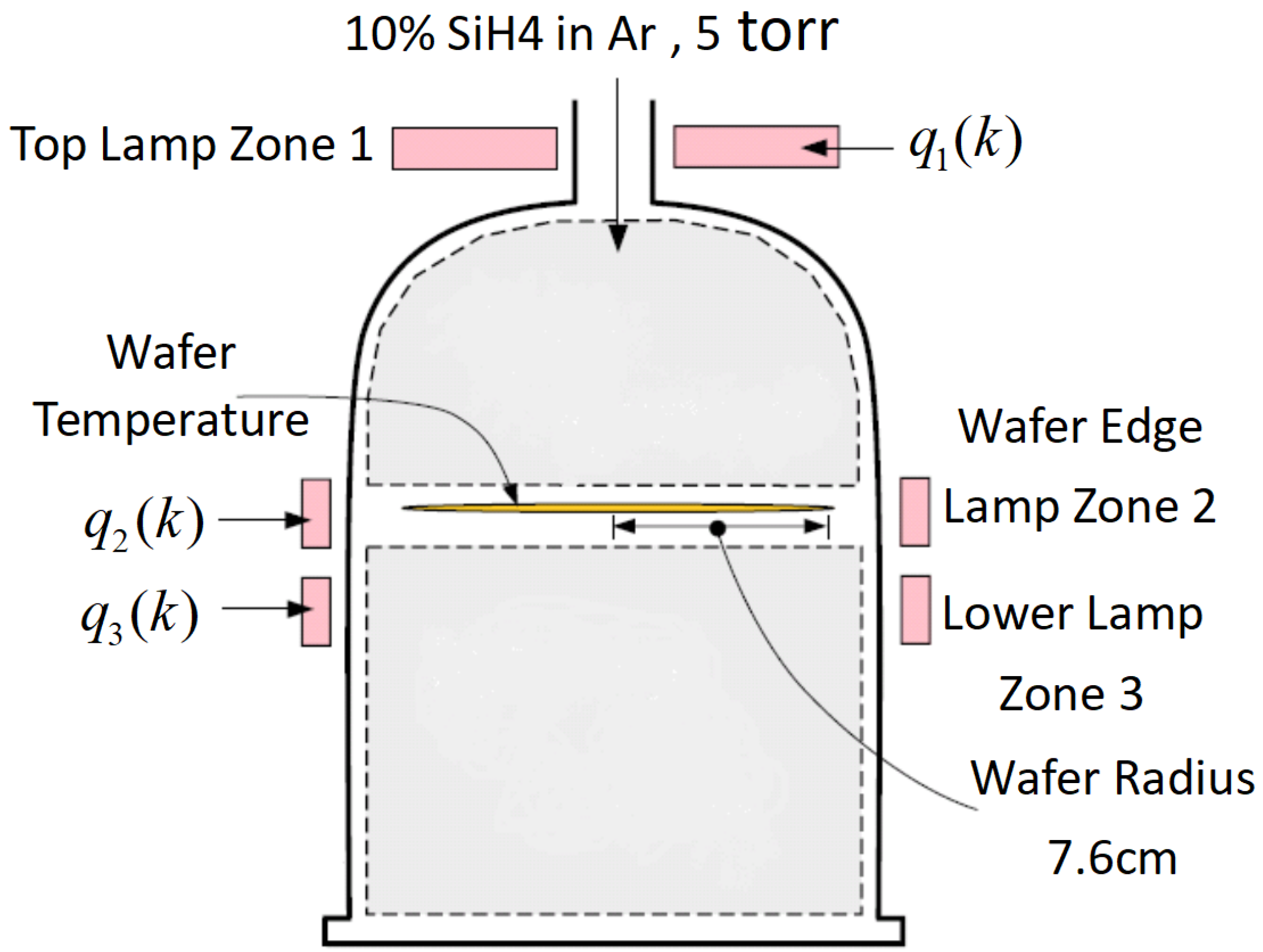
Figure 4 displays the schematic of the rapid thermal chemical vapor deposition (RTCVD) system.
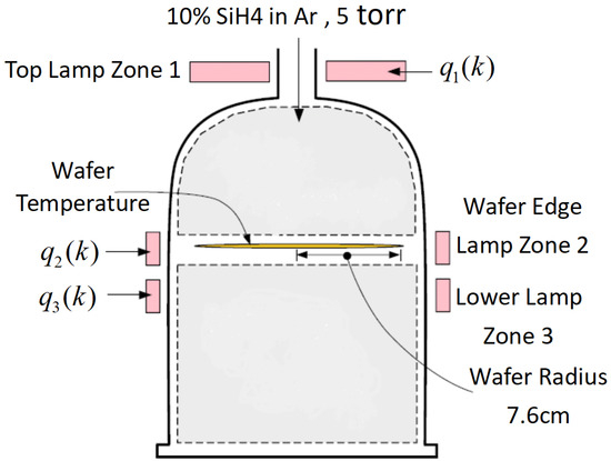
Figure 4.
Sketch for the RTCVD system.
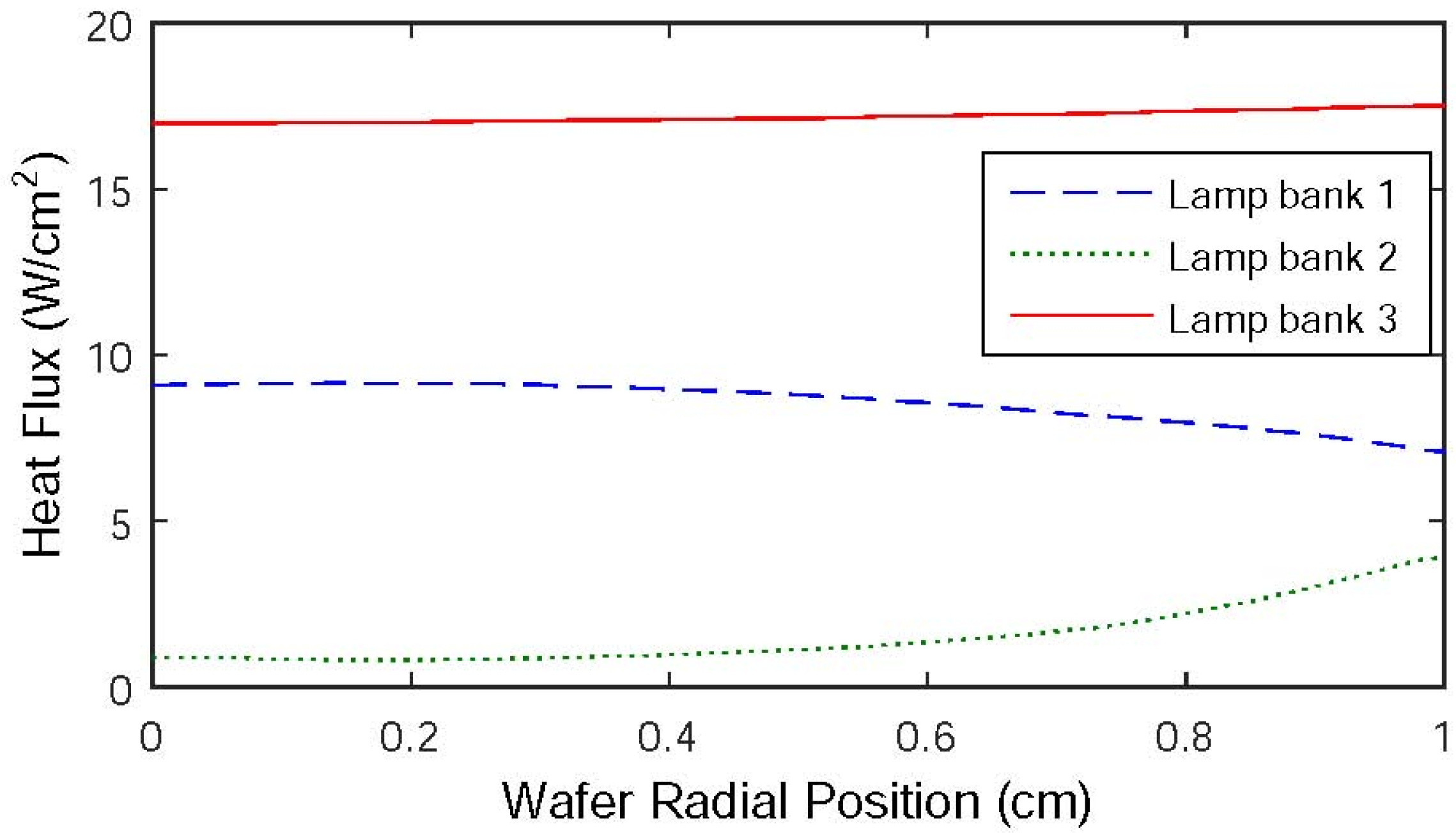
A 6-inch silicon wafer is positioned on a revolving support inside the system’s chamber and subjected to heat from a heating system. The heating system consists of three Lamp banks. Lamp bank 1 uniformly warms the whole surface area of the wafer, Lamp bank 2 specifically heats the periphery of the wafer, and Lamp bank 3 equally heats the wafer as a whole. Figure 5 displays the incident radiation flux emitted by the heating lights. A 10% concentration of silane gas (SiH4) is fed into the reactor. SiH4 undergoes decomposition to produce silicon (Si) and hydrogen gas (H2). A layer of polysilicon, with a thickness of 0.5 m, is applied onto the wafer by depositing it at temperatures of about 800 K or more, which takes about 1 min. During wafer processing, the support is turned to ensure that the temperature is evenly distributed in the azimuthal direction. Due to the thinness of the silicon wafer, all changes in temperature along the azimuth direction are disregarded. Hence, it is necessary to maintain consistent temperature distribution over the wafer radius in order to achieve a homogeneous deposition of polysilicon on the wafer. This may be achieved by regulating the power supplied to the three zones of lighting groups. A one-dimensional space model of the thermal dynamics may be expressed as the following PDE [25,26]:
This is constrained by the specified border conditions:
where the nondimensional wafer temperature, denoted by , represents the ratio of the actual wafer temperature to the ambient temperature , which is 300 K. The nondimensional time, denoted by , represents the ratio of the actual time to , which is 2.9 s. The nondimensional radius position, denoted by , represents the ratio of the actual radius position to the wafer radius , which is 7.6 cm. The variables , , and represent the percentage of the light source power. The variables , , and represent the wafer incident radiation flux from the three-zone warming lights, respectively. The parameters in (17) through (18) are listed as follows:
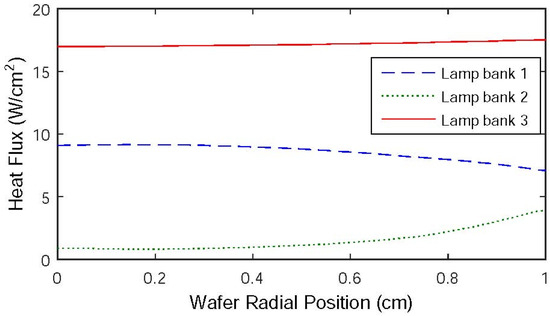
Figure 5.
Radiation flux distribution of Lamp banks 1, 2, and 3.
The RTCVD system is a complex system that exhibits both spatial and temporal characteristics and has an unlimited number of dimensions. For practical purposes, a certain number of sensors must be used. Assume that sensors positioned at are employed to gauge the system’s output. Consider to be the spatial domain, where is a vector containing the elements . Let be a vector denoted by , where . The temporal input is defined as , where is the time variable. The objective of the modeling problem is to determine a spatiotemporal model based on the input and the output , where K represents the duration of time. The mechanism model of RTCVD described above is used to simulate the real systems and generate data for establishing a 3D fuzzy model. In this paper, we use Matlab 2022b software to realize the simulation of RTCVD, the realization of 3D fuzzy modeling (including clustering analysis and SPSA algorithm), and the comparison of different modeling methods.
In practical operation, 11 sensors are placed evenly along the radial direction. To simulate the impact of noise, 11 independent sets of Gaussian white noise signals are added to the data collected from 11 sensors. The average value is zero, and the standard deviation is , , .
4.2. SPSA Learning-Based Three-Dimensional Fuzzy Modeling
In order to obtain sufficient dynamic information of the system, interference signals with amplitudes not exceeding 10% are added to the manipulated input variables , , and , respectively. Thus, the three manipulated input variables affected by interference signals, namely, the excitation signals, can be given by the following Equation (19):
where , , and are steady-state inputs at a furnace temperature of 1000 K. , , and are the disturbance amplitude of , and . In this study, , , and are 0.2028, 0.1008, and 0.2245, respectively, and , , and are set to .
A sample interval of 0.5 s was established in this investigation. The entire simulation time period was 7000 s. Therefore, 14,000 samples were generated, in which 600 samples were randomly selected for training experiments, and then 300 samples were randomly selected for test experiments.
In this study, for simplicity, and were chosen. Thus, the data set can be written as Equation (20):
where
For in the data set S, AP clustering is used. The AP method sets the coefficient of dampness to 0.9 and the reference degree P to 0.5. Following the process of clustering learning, a total of seven fuzzy rules and their accompanying clustering cores were successfully acquired. Equation (7) shows the breadth setting of the Gaussian spatial membership function, whereas Equation (8) shows the breadth setting of the conventional Gaussian membership function.
This paper uses Fourier space base functions to represent the fuzzy rule resulting sets, and applies the SPSA method to improve the coefficients of Fourier space base functions.
In the SPSA algorithm, the relevant parameter settings are as follows: , , , , , and .
Based on the learning results of the AP algorithm, it is evident that there are a total of seven fuzzy rules, so the parameter dimension that needs to be adjusted is 28, and the optimization range control of the parameters is . The end point criterion is defined as either reaching the maximum number of iterations or when the change in iteration becomes less than 0.00001 for five consecutive occasions.
The initial value of is obtained through the gradient descent algorithm as shown in Equation (21):
By using the SPSA algorithm, the optimal parameters for the Fourier space base function of the fuzzy rule resulting set can be obtained.
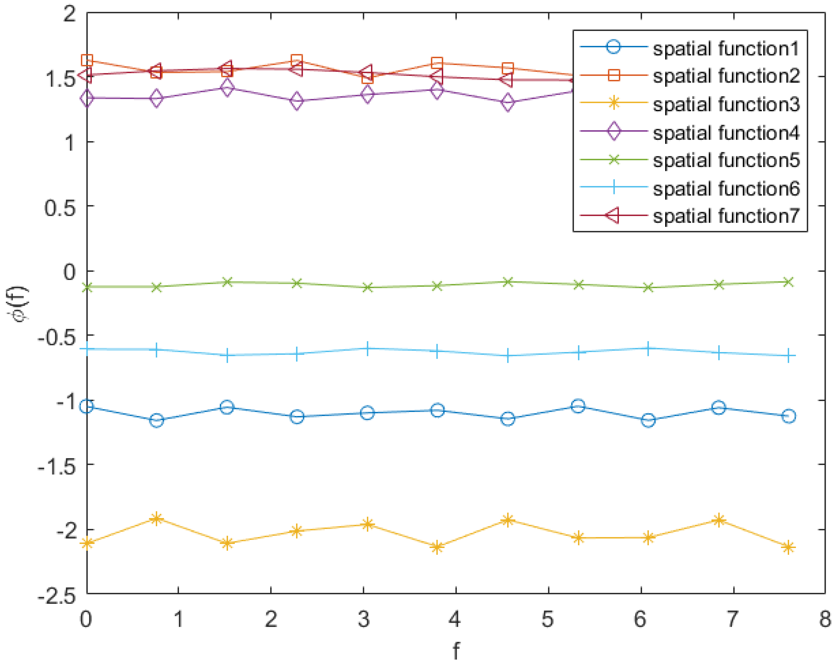
For the convenience of observation, Figure 6 shows seven space base functions.
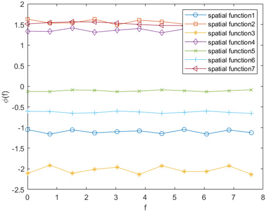
Figure 6.
Seven space base functions learned by the SPSA algorithm.
The seven three-dimensional fuzzy rules derived from the data are listed as follows:
if is very Positive Large and is Positive Small and is Positive Large and is very Positive Large, then is [0.8147 0.9058 0.1270 0.9134 0.6324 0.0975 0.2785 0.5469 0.9575 0.9649 0.1576].
if is more than Zero and is less than Positive Medium and is Positive Small and is Positive Medium, then is [6.7941 6.7002 3.3976 5.6020 0.9932 2.9523 6.4101 5.5455 6.7164 4.5902 0.2500].
if is less than Positive Small and is more than Positive Medium and is more than Zero and is very Positive Large, then is [12.7369 −14.0099 −10.1810 −11.3661 −11.1470 −5.8834 −9.8322 −2.5678 −10.5907 −0.4775 −4.1538].
if is very Positive Large and is Positive Large and is slightly Positive Small and is Positive Large, then is [0.4617 0.9713 8.2346 6.9483 3.1710 9.5022 0.3445 4.3874 3.8156 7.6552 7.9520].
if is more than Positive Medium and is Positive Large and is more than Zero and is Positive Medium, then is [1.8687 4.8976 4.4559 6.4631 7.0936 7.5469 2.7603 6.7970 6.5510 1.6261 1.1900].
if is more than Positive Medium and is Positive Medium and is slightly Positive Small and is very Positive Large, then is [−2.4918 −4.7987 −1.7019 −2.9263 −1.1191 −3.7563 −1.2755 −2.5298 −2.5673 −2.3571 −3.125].
if is Positive Large and is Positive Small and is Positive Small and is less than Positive Medium, then is [−1.2263 −0.4110 −1.1889 −0.7443 −1.0026 −0.4407 −1.3535 −1.6484 −2.6840 −1.4376 −0.6583].
Finally, the complete three-dimensional fuzzy modeling of RTCVD is achieved. The abbreviation for the suggested three-dimensional modeling technique, which combines AP clustering with Fourier space base functions, is AP-Fourier-SPSA-3D fuzzy modeling.
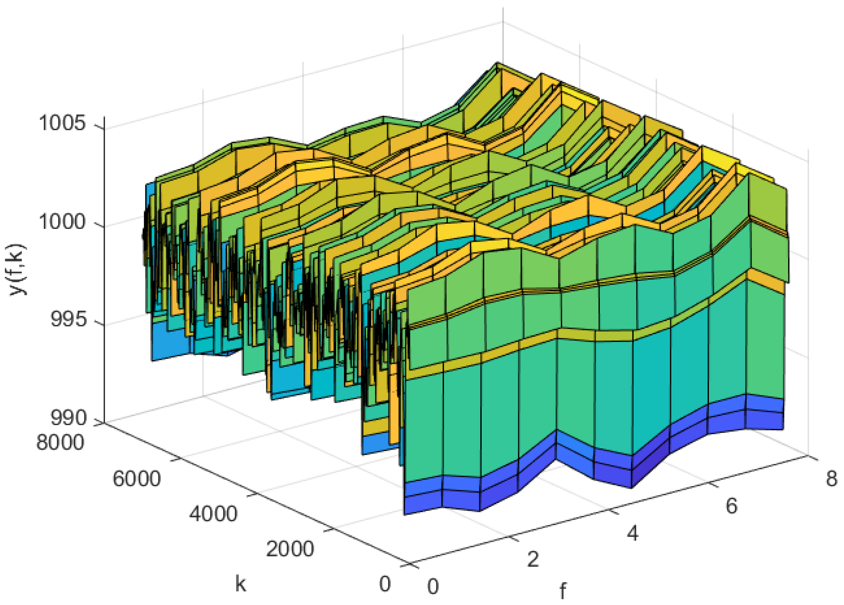
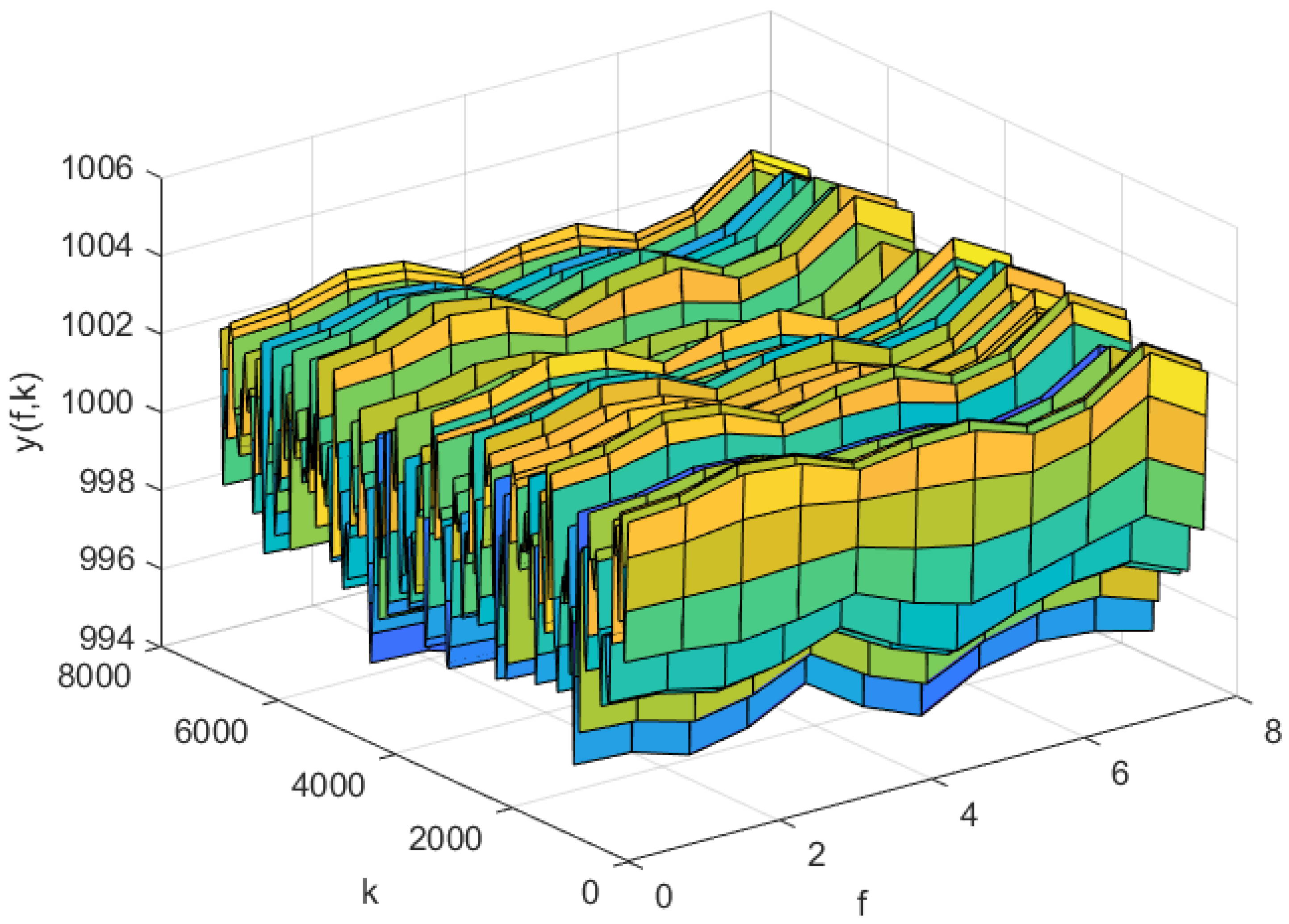
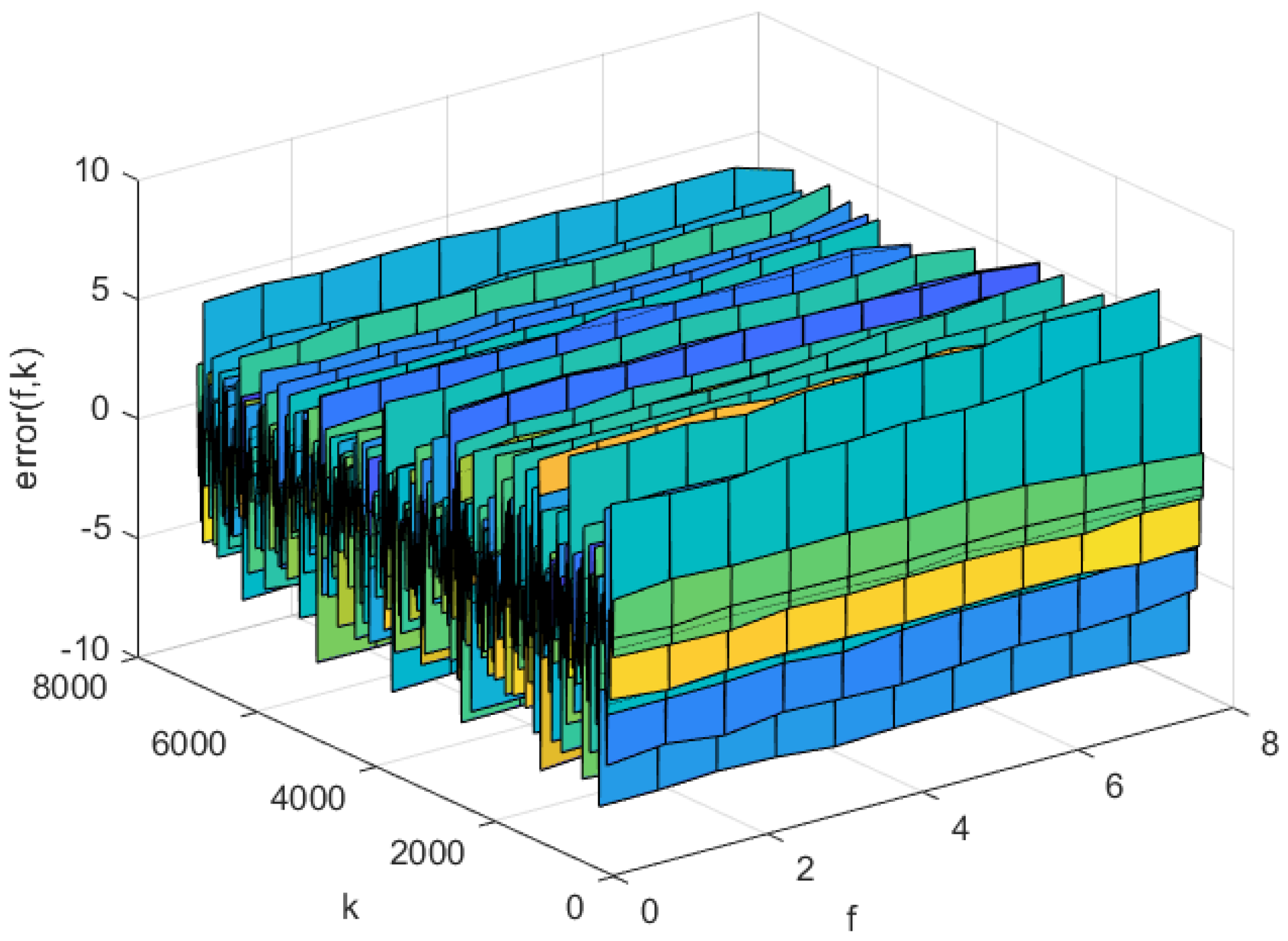
The simulation results of AP-Fourier-SPSA-3D are shown in the following figures. The predicted result of the model in the training data is displayed in Figure 7, while the discrepancies between the expected and actual values are illustrated in Figure 8. Figure 9 displays the anticipated outcome of the procedure in the test data, whereas Figure 10 illustrates the flaws in the predictions. The root mean square error (RMSE) performance indices are shown in Table 1.

Figure 7.
The predicted process output of the AP-Fourier-SPSA-3D model in the training data.
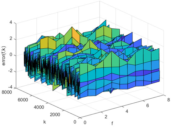
Figure 8.
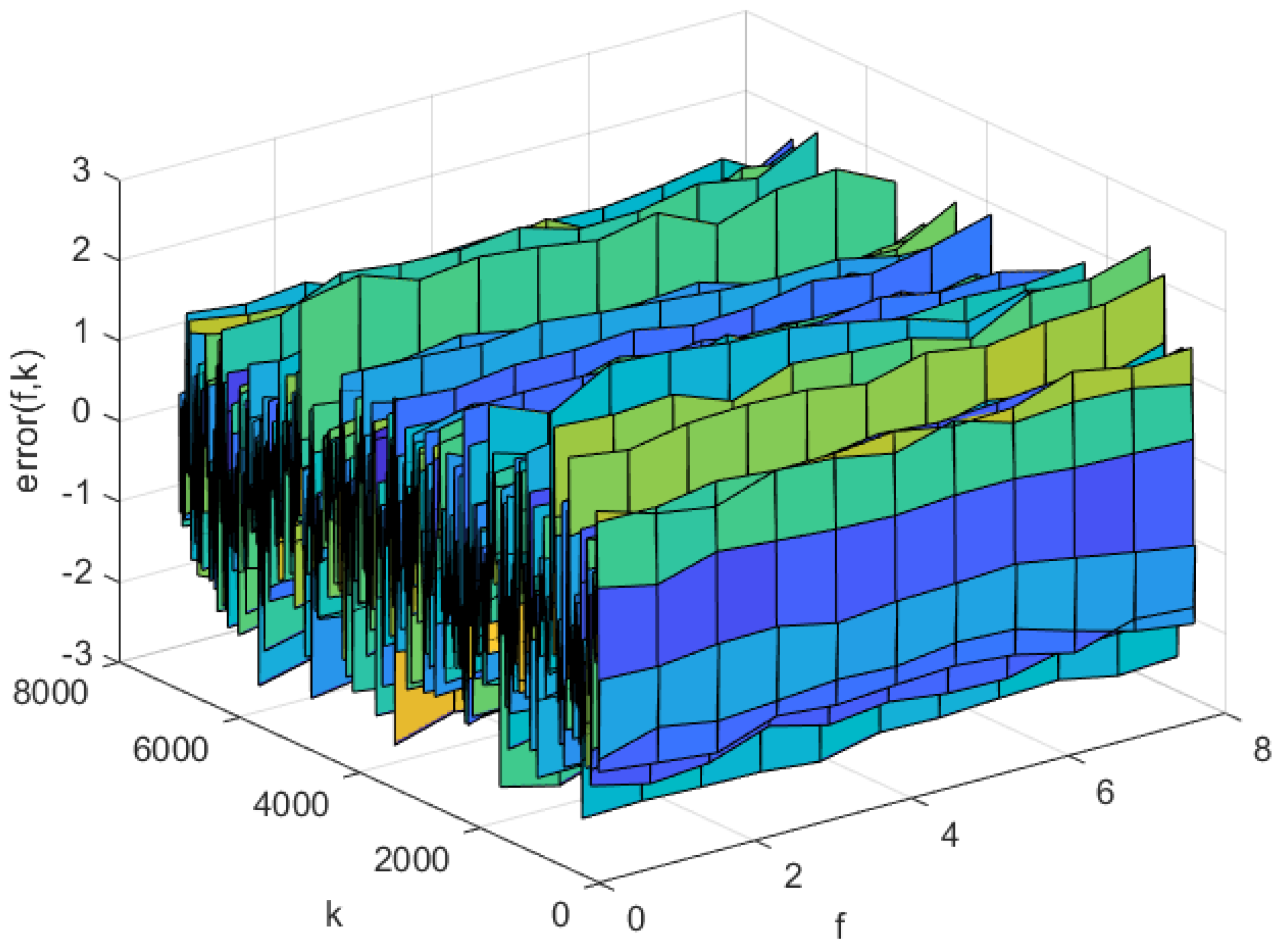
The predicted errors of the AP-Fourier-SPSA-3D model in training data.

Figure 9.
The predicted process output of the AP-Fourier-SPSA-3D model in test data.
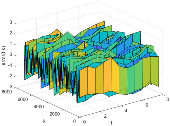
Figure 10.
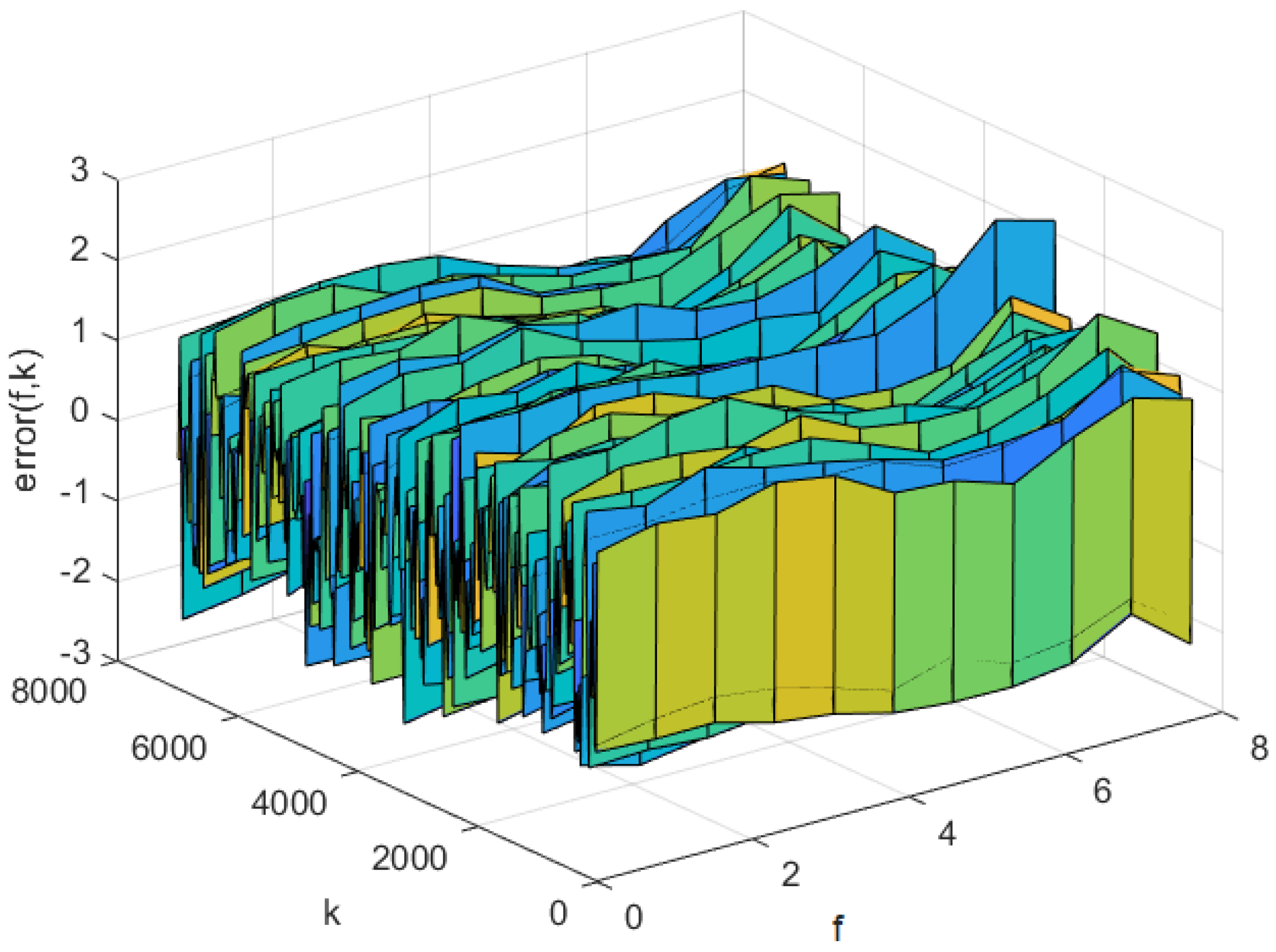
The predicted errors of the AP-Fourier-SPSA-3D model in test data.

Table 1.
Comparison of RMSE among AP-Fourier-SPSA-3D, AP-Fourier-GD-3D, NNC-SVR-3D and KL-LS.
4.3. Simulation Comparison
In this study, two modeling methods were selected for comparison: KL-LS [27] and NNC-SVR-3D [10]. The KL-LS modeling approach utilizes the KL decomposition technique to compute space functions and decrease model dimensions. Subsequently, the least squares identification method is employed to determine low-dimensional temporal coefficients. The NNC-SVR-3D fuzzy modeling method uses the nearest neighbor clustering algorithm to learn the preceding components of three-dimensional fuzzy rules, which is reduced with the use of a similarity assessing approach, and uses multiple single-output support vector machines to learn the space base functions of the resulting components. Additionally, the gradient descent approach is utilized to determine the coefficients of Fourier space base functions for the suggested three-dimensional fuzzy modeling based on AP clustering and the Fourier space base function, which is abbreviated as AP-Fourier-GD-3D.
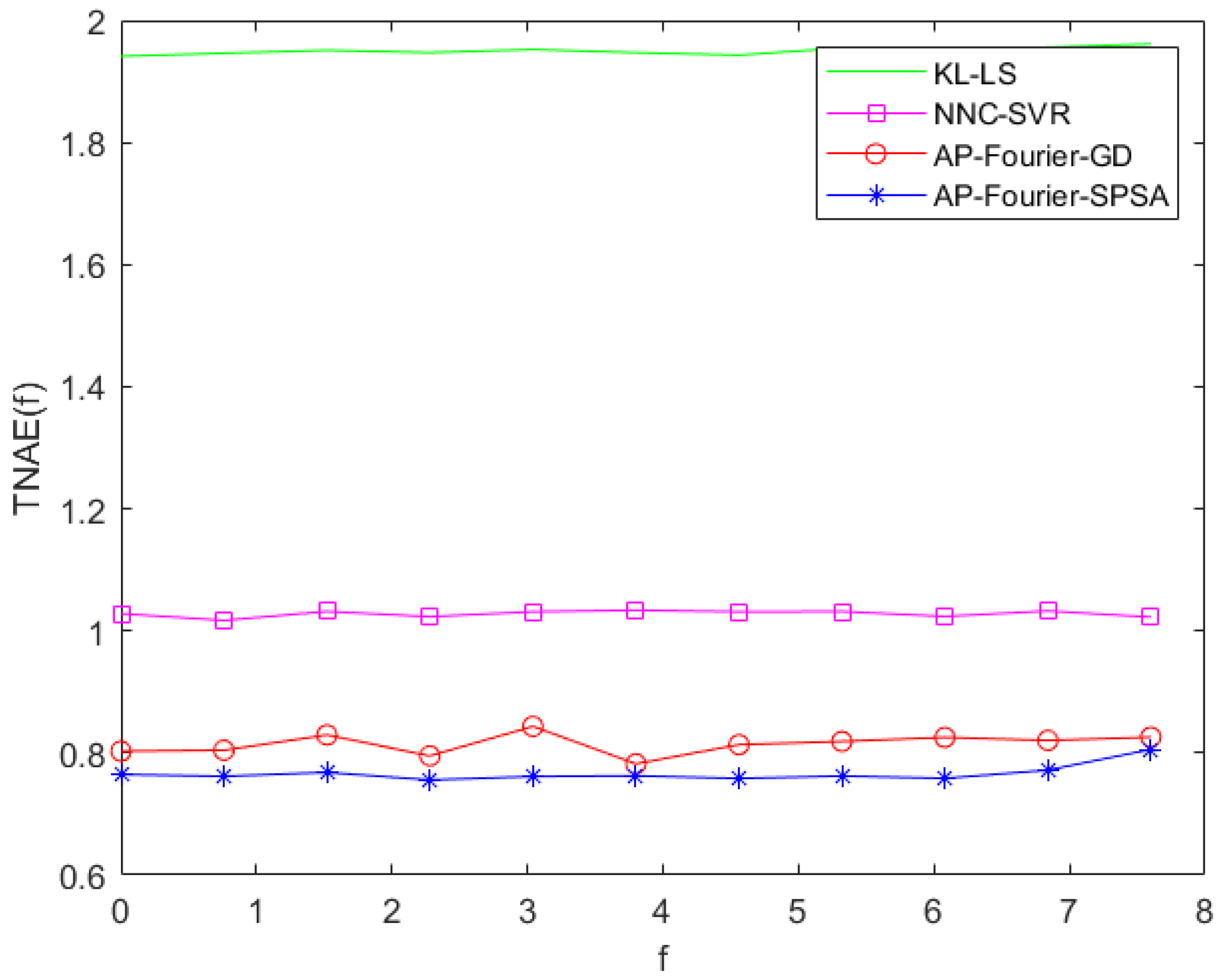
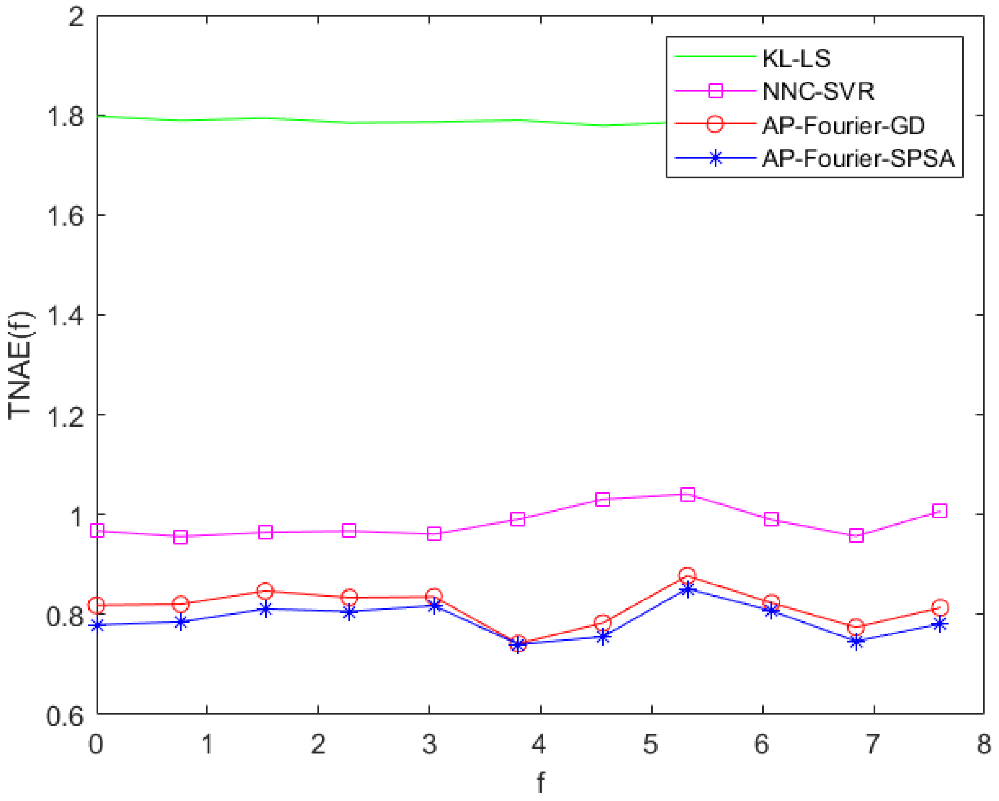
The prediction errors of the KL-LS model and the NNC-SVR model on the training data and test data can be seen in Figure 11 and Figure 12, and Figure 13 and Figure 14, respectively. The time normalized absolute errors of these models on training and test data are shown in Figure 15 and Figure 16, respectively. The RMSE performance indexes of these models are shown in Table 1.

Figure 11.
Prediction error of the KL-LS model on the training set.
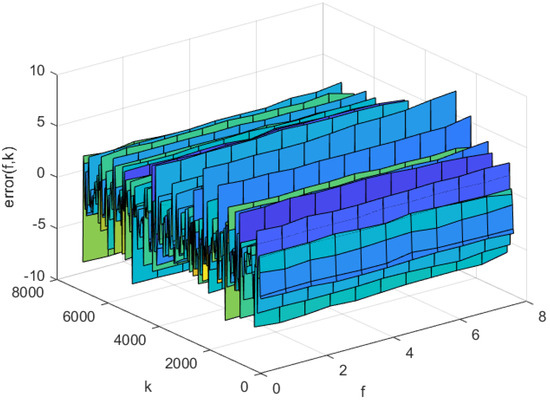
Figure 12.
Prediction error of the KL-LS model on the test set.

Figure 13.
Prediction error of the NNC-SVR-3D model on the training set.

Figure 14.
Prediction error of the NNC-SVR-3D model on the test set.
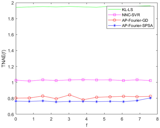
Figure 15.
TNAE of the four models on the training data.
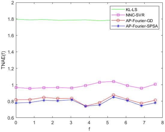
Figure 16.
TNAE of the four models on the test data.
From Table 1 and Figure 7, Figure 8, Figure 9, Figure 10, Figure 11, Figure 12, Figure 13, Figure 14, Figure 15 and Figure 16, it is evident that the three-dimensional fuzzy models outperform the KL-LS model. The KL-LS modeling method is traditional modeling methods based on KL decomposition, which require dimension reduction. Consequently, this will unavoidably result in the emergence of unmodeled dynamic characteristics and uncertainties. The suggested three-dimensional modeling approach seamlessly merges space–time separation and space–time reconstruction, eliminating the necessity of reducing dimensions. In three three-dimensional fuzzy models, the proposed AP-Fourier-SPSA-3D model has better performance. It discloses that the Fourier space base function has better spatial characteristics to disclose the spatial relationship of the DPS system, the AP clustering algorithm can adaptively select cluster cores and its numbers based on the distribution characteristics of data, and the SPSA algorithm can successfully avoid becoming stuck in the local optima.
5. Conclusions
The study introduced a novel three-dimensional fuzzy modeling technique using SPSA learning for DPS, which widely exists in the manufacturing industry. On the three-dimensional fuzzy modeling framework, AP clustering was used to learn the preceding components and adaptively determine the quantity of fuzzy rules. The three-dimensional fuzzy model used the Fourier space base functions as the resulting components, while the SPSA method was employed to dynamically acquire the coefficients of the Fourier space base functions. The suggested approach was implemented on a conventional distributed parameter system in the semiconductor manufacturing industry. The simulation experiment demonstrates the superiority of the three-dimensional fuzzy modeling method over the conventional space–time separation modeling method. Additionally, it shows that the Fourier space base function is more effective in revealing the spatial distribution characteristics of distributed parameter systems compared to the spatial function obtained through KL decomposition.
The three-dimensional fuzzy modeling framework is an intelligent modeling framework for spatiotemporal coupled systems. Under this framework, the commonly used machine learning methods (such as clustering analysis, support vector machine, least square method, random gradient method, reinforcement learning, etc.) can be applied to learn the preceding components of the fuzzy model and the resulting components of the three-dimensional fuzzy model. In the future research work, we will try to apply reinforcement learning to three-dimensional fuzzy modeling. Through interactive learning with the environment, we can establish an online 3D fuzzy model for a nonlinear distributed parameter system.
Author Contributions
Conceptualization, T.W.; Data curation, S.W.; Formal analysis, C.C.; Funding acquisition, X.Z.; Investigation, C.C.; Methodology, X.Z.; Project administration, X.Z.; Resources, S.W.; Software, T.W.; Supervision, X.Z.; Validation, C.C.; Visualization, S.W.; Writing—original draft, T.W.; Writing—review and editing, X.Z. All authors have read and agreed to the published version of the manuscript.
Funding
This work was supported by the project from the National Natural Science Foundation of China under Grant 62073210.
Institutional Review Board Statement
Not applicable.
Informed Consent Statement
Not applicable.
Data Availability Statement
The original contributions presented in the study are included in the article, further inquiries can be directed to the corresponding author. Dataset available on request from the authors. The raw data supporting the conclusions of this article will be made available by the authors on request.
Conflicts of Interest
Author Chong Cheng was employed by the company China Mobile (Suzhou) Software Technology Co., Ltd. The remaining authors declare that the research was conducted in the absence of any commercial or financial relationships that could be construed as a potential conflict of interest.
Appendix A. Algorithm Description of AP Clustering and Its Flow Chart
AP clustering is a clustering algorithm based on the information propagation between data points. Unlike other clustering algorithms, AP clustering does not require a prespecified number of clusters, and the chosen cluster centers are actual points within the data set. The algorithm operates by using an input similarity matrix S derived from the data, where represents the suitability of data point v as a potential cluster center for data point i.
During the iterative process, the algorithm propagates two types of information, responsibility and availability, as depicted in Figure A1. In Figure A1, each is represented by a function node, and each is represented by a variable node. Each is connected to all variable nodes , and each is connected to its corresponding single node. The information propagation process is illustrated in Figure A2. Responsibility is conveyed from data point i to exemplar v, reflecting the degree to which v is a credible cluster center for i, while taking into account other exemplars. Availability is conveyed from exemplar v to data point i, representing the likelihood that v will be selected as the cluster center for i, considering the support from other data points for v [28].
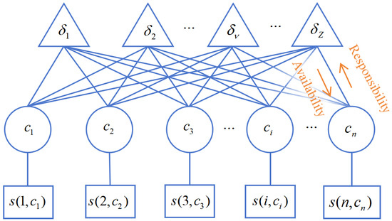
Figure A1.
Affinity Propagation factor graph.
Figure A1.
Affinity Propagation factor graph.

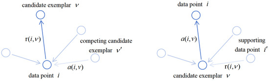
Figure A2.
The direction of the passing message.
Figure A2.
The direction of the passing message.
The AP algorithm iteratively updates the responsibility and availability for each data point, with these values collectively determining whether a sample can become an exemplar, thereby leading to the final clustering results.
Assume that is a data set, (). The procedure of AP clustering is described as given below, and its process diagram is displayed in Figure A3.
Figure A3.
Flow chart of the AP clustering algorithm.
Figure A3.
Flow chart of the AP clustering algorithm.
Step 1: Calculate the similarity matrix S of the data pair. The similarity between any two sample points and is measured by the negative Euclidean distance: . Then, the similarity matrix S is normalized as in (A1)
Step 2: Set the maximum number of iteration T, damping factor , and reference degree .
Step 3: Update the responsibility matrix, and the update rule is given as follows:
Using damping factor , the responsibility matrix at the kth iteration is updated as in (A4):
Step 4: Update the availability matrix, and the update rules are given as follows:
Using damping factor , the availability matrix at the jth iteration is updated as in (A7):
Step 5: The decision matrix is obtained by summing the availability matrix and the responsibility matrix. Find the point in the decision matrix where the diagonal is greater than 0 as the cluster representative center. The sample points are classified according to the distance between the sample points and the cluster representative points.
Step 6: Determine the number of iterations and the iteration stop condition. The current iteration number has reached the set maximum iteration number T, or the current iteration number is less than T, but the change in its class representative center after several iterations is less than a small value, the AP clustering algorithm ends the iteration, and we assign the data points to the corresponding cluster centers.
Although the AP clustering algorithm does not require specifying the number of clusters explicitly, there are some key clustering parameters, namely, the reference value P and the damping factor [29].
- Reference value is the degree to which point v is considered a cluster center, and it corresponds to the diagonal values of the similarity matrix S. The reference value directly affects the number of clusters obtained and the choice of cluster centers. A higher reference value indicates a higher likelihood that a data point will become a cluster center; conversely, a lower reference value reduces the likelihood of a data point being chosen as a cluster center. In the absence of prior knowledge, the median of similarity values is typically used as the reference value for each data point, generally ranging between [0, 1]. In this study, a reference value of 0.5 is used and set as a global shared preference.
- Damping factor is introduced to prevent data oscillations during the information propagation process. A higher damping factor limits the magnitude of updates during iterations, thus enhancing algorithm stability but slowing convergence. Conversely, a lower damping factor accelerates convergence but may lead to more oscillations. Based on expert experience, common settings for the damping factor are 0.5 or 0.9. In this study, a damping factor of 0.9 is used.
References
- Christofides, P.D.; Chow, J. Nonlinear and Robust Control of PDE Systems: Methods and Applications to Transport-Reaction Processes. Appl. Mech. Rev. 2002, 55, B29–B30. [Google Scholar] [CrossRef]
- Wang, Z.P.; Wu, H.N.; Chadli, M. H∞ Sampled-Data Fuzzy Observer Design for Nonlinear Parabolic PDE Systems. IEEE Trans. Fuzzy Syst. 2020, 29, 1262–1272. [Google Scholar] [CrossRef]
- Braess, D.; Schumaker, L.L. Finite Elements: Theory, Fast Solvers, and Applications in Elasticity Theory; Cambridge University Press: Cambridge, UK, 2007. [Google Scholar]
- Lu, X.J.; Zou, W.; Huang, M.H. A Novel Spatiotemporal LS-SVM Method for Complex Distributed Parameter Systems with Applications to Curing Thermal Process. IEEE Trans. Ind. Inf. 2016, 12, 1156–1165. [Google Scholar] [CrossRef]
- Wang, M.L.; Li, N.; Li, S.Y. Model-Based Predictive Control for Spatially-Distributed Systems Using Dimensional Reduction Models. Int. J. Autom. Comput. 2011, 8, 1–7. [Google Scholar] [CrossRef]
- Huang, K.; Tao, S.; Wu, D.; Yang, C.; Gui, W. Physical Informed Sparse Learning for Robust Modeling of Distributed Parameter System and Its Industrial Applications. IEEE Trans. Automat. Sci. Eng. 2023, 21, 4561–4572. [Google Scholar] [CrossRef]
- Li, H.X.; Qi, C.K. Modeling of Distributed Parameter Systems for Applications—A Synthesized Review from Time-Space Separation. J. Process Control 2010, 20, 891–901. [Google Scholar] [CrossRef]
- Li, H.X.; Qi, C.K. Spatio-Temporal Modeling of Nonlinear Distributed Parameter Systems: A Time/Space Separation Based Approach; Springer Science & Business Media: Berlin, Germany, 2011. [Google Scholar]
- Fan, Y.J.; Xu, K.K.; Wu, H.; Zheng, Y.; Tao, B. Spatiotemporal Modeling for Nonlinear Distributed Thermal Processes Based on KL Decomposition, MLP and LSTM Network. IEEE Access 2020, 8, 25111–25121. [Google Scholar] [CrossRef]
- Zhang, X.X.; Zhao, L.R.; Li, H.X.; Ma, S.W. A Novel Three-Dimensional Fuzzy Modeling Method for Nonlinear Distributed Parameter Systems. IEEE Trans. Fuzzy Syst. 2019, 27, 489–501. [Google Scholar] [CrossRef]
- Wang, M.L.; Qi, C.K.; Yan, H.C.; Shi, H.B. Hybrid Neural Network Predictor for Distributed Parameter System Based on Nonlinear Dimension Reduction. Neurocomputing 2016, 171, 1591–1597. [Google Scholar] [CrossRef]
- Zhang, R.D.; Tao, J.L.; Lu, R.Q.; Jin, Q.B. Decoupled ARX and RBF Neural Network Modeling Using PCA and GA Optimization for Nonlinear Distributed Parameter Systems. IEEE Trans. Neural Netw. Learn. Syst. 2016, 29, 457–469. [Google Scholar] [CrossRef]
- Wang, Y.; Li, H.-X.; Yang, H. Adaptive Spatial-Model-Based Predictive Control for Complex Distributed Parameter Systems. Adv. Eng. Inform. 2024, 59, 102331. [Google Scholar] [CrossRef]
- Chen, L.; Shen, W.; Zhou, Y.; Mou, X.; Lei, L. Learning-Based Sparse Spatiotemporal Modeling for Distributed Thermal Processes of Lithium-Ion Batteries. J. Energy Storage 2023, 69, 107834. [Google Scholar] [CrossRef]
- Jin, X.; Wu, D.; Yang, H.; Zhu, C.; Shen, W.; Xu, K. A Temporal–Spatiotemporal Domain Transformation-Based Modeling Method for Nonlinear Distributed Parameter Systems. J. Comput. Des. Eng. 2023, 10, 1267–1279. [Google Scholar] [CrossRef]
- Zhang, X.X.; Fu, Z.Q.; Li, S.Y.; Zou, T.; Wang, B. A Time/Space Separation Based 3D Fuzzy Modeling Approach for Nonlinear Spatially Distributed Systems. Int. J. Autom. Comput. 2018, 15, 52–65. [Google Scholar] [CrossRef]
- Deng, H.; Li, H.X.; Chen, G. Spectral-Approximation-Based Intelligent Modeling for Distributed Thermal Processes. IEEE Trans. Control Syst. Technol. 2005, 13, 686–700. [Google Scholar] [CrossRef]
- Meng, X.B.; Chen, C.L.P.; Li, H.X. Confidence-Aware Multiscale Learning for Online Modeling of Distributed Parameter Systems with Application to Curing Process. IEEE Trans. Ind. Electron. 2023, 70, 9432–9440. [Google Scholar] [CrossRef]
- Wei, P.; Li, H.X. Two-Dimensional Spatial Construction for Online Modeling of Distributed Parameter Systems. IEEE Trans. Ind. Electron. 2022, 69, 10227–10235. [Google Scholar] [CrossRef]
- Feng, Y.; Zhu, X.Y.; Wang, Y.N.; Wang, B.C.; Zhang, H.; Wu, Z.G.; Yan, H.C. PDE Model-Based On-Line Cell-Level Thermal Fault Localization Framework for Batteries. IEEE Trans. Syst. Man Cybern. Syst. 2024, 54, 2507–2516. [Google Scholar] [CrossRef]
- Li, H.X.; Zhang, X.X.; Li, S.Y. A Three-Dimensional Fuzzy Control Methodology for a Class of Distributed Parameter Systems. IEEE Trans. Fuzzy Syst. 2007, 15, 470–481. [Google Scholar] [CrossRef]
- Zhang, X.X.; Jiang, Y.; Li, H.X.; Li, S.Y. SVR Learning-Based Spatiotemporal Fuzzy Logic Controller for Nonlinear Spatially Distributed Dynamic Systems. IEEE Trans. Neural Netw. Learn. Syst. 2013, 24, 1635–1647. [Google Scholar] [CrossRef]
- Frey, B.J.; Dueck, D. Clustering by Passing Messages Between Data Points. Science 2007, 315, 972–976. [Google Scholar] [CrossRef] [PubMed]
- Spall, J.C. Introduction to Stochastic Search and Optimization: Estimation, Simulation, and Control; John Wiley & Sons: Hoboken, NJ, USA, 2005. [Google Scholar]
- Theodoropoulou, A.; Adomaitis, R.A.; Zafiriou, E. Model Reduction for Optimization of Rapid Thermal Chemical Vapor Deposition Systems. IEEE Trans. Semicond. Manuf. 1998, 11, 85–98. [Google Scholar] [CrossRef]
- Adomaitis, R.A. A Reduced-Basis Discretization Method for Chemical Vapor Deposition Reactor Simulation. Math. Comput. Model. 2003, 38, 159–175. [Google Scholar] [CrossRef]
- Qi, C.K.; Li, H.-X. A Karhunen-Loève Decomposition-Based Wiener Modeling Approach for Nonlinear Distributed Parameter Processes. Ind. Eng. Chem. Res. 2008, 47, 4184–4192. [Google Scholar] [CrossRef]
- Jiao, L.; Bie, R.; Zhang, G.; Wang, S.; Mehmood, R. Proper Global Shared Preference Detection Based on Golden Section and Genetic Algorithm for Affinity Propagation Clustering. Int. J. Distrib. Sens. Netw. 2016, 12, 1–10. [Google Scholar] [CrossRef]
- Moiane, A.F.; Machado, A.M.L. Evaluation of the Clustering Performance of Affinity Propagation Algorithm Considering the Influence of Preference Parameter and Damping Factor. Bol. Ciênc. Geodés. 2018, 24, 426–441. [Google Scholar] [CrossRef]


Disclaimer/Publisher’s Note: The statements, opinions and data contained in all publications are solely those of the individual author(s) and contributor(s) and not of MDPI and/or the editor(s). MDPI and/or the editor(s) disclaim responsibility for any injury to people or property resulting from any ideas, methods, instructions or products referred to in the content. |
© 2024 by the authors. Licensee MDPI, Basel, Switzerland. This article is an open access article distributed under the terms and conditions of the Creative Commons Attribution (CC BY) license (https://creativecommons.org/licenses/by/4.0/).