Modeling and Multi-Objective Optimization Design of High-Speed on/off Valve System

Abstract

The design of the high-speed on/off valve is challenging due to the interrelated structural parameters of its driving actuator. Hence, this study proposes a multi-objective optimization approach that integrates a backpropagation neural network and artificial fish swarm algorithm optimization techniques to accurately model the electromagnetic solenoid structure. The backpropagation neural network is fitted and trained using simulation data to obtain a reduced-order model of the system, enabling the precise prediction of the system’s output based on the input structural parameters. By employing the artificial fish swarm algorithms, with optimization objectives focusing on the valve’s opening and closing times, a Pareto optimal solution set comprising 30 solutions is generated. Utilizing the optimized structural parameters, a prototype is manufactured and an experimental setup is constructed to verify the dynamic characteristics and flow pressure drop. The high-speed on/off valve achieves an approximate opening and closing time of 3 ms. Notably, the system output predicted using the backpropagation neural network (BPNN) exhibits consistency with the experimental findings, providing a reliable alternative to mathematical modeling.

1. Introduction

Traditional electro-hydraulic servo systems typically utilize servo or proportional valves as control components. These valves offer numerous advantages, including excellent accuracy, low hysteresis, and minimal dead zone, which contribute to improved control function. However, servo valves also suffer from certain drawbacks, such as high cost, poor efficiency, and reduced reliability due to their sensitivity to the contamination of transmission media [1]. Consequently, the replacement of servo valves with a combination of high-speed on/off valves (HSV) in digital hydraulic systems has emerged as a growing trend [2]. HSVs constantly operate in fully open or fully closed states, effectively discretizing continuous flow and serving as the fundamental components of digital hydraulic systems [3]. Over the past years, digital hydraulic components have obtained extensive traction in the hydraulic systems field due to their ability to be directly controlled by pulse width modulation signals [4]. The integration of digital hydraulic systems can significantly enhance overall efficiency, making HSVs a prominent research focus in the hydraulic domain [5,6]. Nevertheless, further advancements are required for HSVs to fulfill the demands of digital hydraulic servo systems, particularly in terms of achieving quicker response times, smaller physical dimensions, and higher flow capacities.

In the research on the optimal design of HSV, Yue et al. [7] introduced positive and negative pulse voltage control to the coil of screw-in cartridge valves (SCV), enabling SCVs to replace HSVs in certain application areas without changing their structure. Zhang et al. [8] utilized current feedback analysis based on critical switching currents to estimate the operating state of HSVs, thereby improving their dynamic performance. Wang et al. [9] designed a novel flat-plate HSV spool structure and established a flow field model for the flat-plate spool, enhancing HSVs’ flow field stability and flow rate. Yang et al. [10] proposed a conical armature structure design and a dual-duty cycle pulse width modulation control method to improve HSVs’ steady-state and transient characteristics. Feng et al. [11] established an HSV parameter analysis model based on the electromagnetic mechanism of solenoid valves to improve HSVs’ dynamic response performance under varying operating conditions. Yang et al. [12] introduced a double magnetic circuit-driven fast on/off valve (DAFV) with a multi-stage excitation control algorithm (MSEC), improving the stability of the HSV response time. Chu et al. [13] developed a pre-excitation control algorithm that allows the coil current to quickly maintain a desired state, thereby enhancing the dynamic performance of HSVs. These studies demonstrate that the primary goal of HSV optimization design is to improve its dynamic characteristics, specifically the response time for valve working.

The interrelationships among various design parameters of HSVs necessitate a comprehensive consideration of each relevant factor during the design process to achieve optimal performance [14]. This complexity gives rise to a multi-objective optimization problem (MOO). Optimization algorithms are commonly utilized to address complex MOO problems, with metaheuristic methods being widely employed in the field of engineering. Metaheuristic algorithms are algorithmic frameworks that operate independently of the specific problem and draw inspiration from natural phenomena, biological behavior, or even mathematics [15]. Metaheuristic methods offer advantages such as randomness, ease of implementation, and the ability to handle black box functions, enabling them to effectively solve a wide range of complex engineering problems [16,17].

Among the numerous metaheuristic algorithms, the artificial fish swarm algorithm (AFSA) has recently garnered significant attention in the literature [18]. The AFSA is a population-based intelligent optimization algorithm, fundamentally inspired by the follow, swarm, prey, and random behaviors of fish [19,20,21]. This algorithm is applicable to various continuous and combinatorial optimization problems. Suppose an artificial fish is currently in state Z, with a visual field set to V, and at a given moment, its viewed position is Zv. If the state at the viewed position is better than the current state of the artificial fish, the fish can move one step towards Zn; otherwise, it continues to search within its visual field for other positions. The perception ability of artificial fish to the surrounding environment increases with the number of explorations, and the improvement of perception ability can help AF make the next decision.

The optimization design of HSVs remains a highly challenging process, primarily due to the dependence of metaheuristic optimization algorithms on accurate system modeling. HSV systems exhibit highly nonlinear characteristics, even without considering the influence of driving circuits, and can be modeled as third-order systems [22]. Precisely predicting the opening and closing time presents significant difficulties. Currently, to conserve computing resources, the widely accepted approach involves approximating functions, making it challenging to achieve high accuracy [23]. In recent years, advanced artificial intelligence methods, particularly those based on neural networks, have made significant advancements and found applications in various fields. Neural network-based methods allow for the direct establishment of black box models by mapping system-related parameters through the training process [24]. Given their strong generalization ability and high prediction accuracy, backpropagation neural networks (BPNN) are an ideal choice for fitting HSV systems [25].

The purpose of this study is to design and validate an HSV model with a permanent magnet structure, focusing on the key performance indicators of rapid opening and closing. In pursuit of this objective, a novel HSV with a permanent magnet bias structure is proposed. The subsequent sections of this paper are organized as follows: Section 2 introduces the proposed valve structure and utilizes system dynamics software for modeling, whereby various design parameters are incorporated to simulate valve response time and flow rate. Section 3 presents the design of the backpropagation neural network (BPNN) structure, followed by its training using simulation data and an analysis of the training accuracy. Section 4 addresses the multi-objective optimization problem, wherein non-dominant solution set screening and storage are incorporated into the artificial fish swarm algorithms (AFSA) algorithm. The improved AFSA is employed to optimize the design of six key parameters in the HSV, facilitating the attainment of Pareto optimal solutions and enabling the selection of parameters based on engineering requirements. Section 5 validates the proposed valve model through an experimental assessment of switching time and pressure drop. Finally, Section 6 presents the corresponding conclusions.

2. New High-Speed on/off Valve Structure and System Modeling

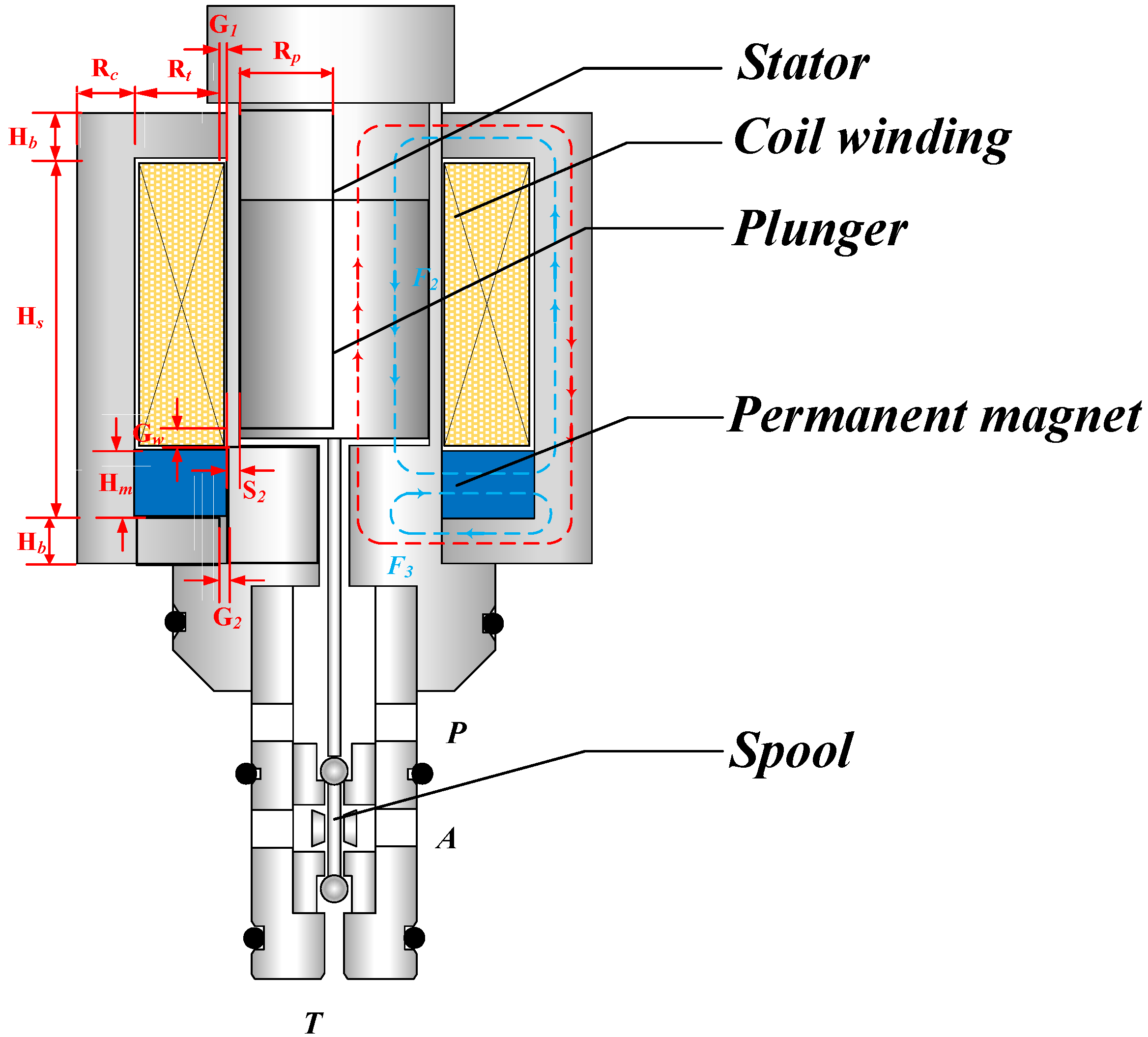
2.1. New High-Speed on/off Valve Structure

The operation of the solenoid valve can be affected by eddy current losses, which have an impact on its performance. In the case of the HSV, these losses primarily occur during the attraction and reset stages of the permanent magnet high-speed solenoid valve, thereby increasing the action time of the HSV. The eddy current losses of the HSV exhibit a positive correlation with the electrical conductivity of the material and a negative correlation with the magnetic saturation intensity [26].

Figure 1 illustrates the structure of the new HSV. At the bottom of the solenoid coil, there is a radially magnetized permanent magnet ring structure. By producing a permanent magnetic field in the reverse direction of the excitation coil at the contact iron, the permanent magnet reduces the magnetic induction intensity throughout the magnetic circuit and prevents magnetic saturation. Furthermore, the use of a low magnetoresistive material with slightly lower saturation magnetic induction and high resistivity for the core, as well as the selection of a low magnetic resistance material for the contact iron, helps minimize eddy current losses. The introduction of the permanent magnet not only reduces the eddy current losses of the contact iron but also enhances the responsiveness of the electromagnetic coil.

The HSV possesses the capability of achieving a three-position, two-way function. In its resting state, the valve remains in a normally closed position, where the high-pressure inlet is designated as the P port and maintains closure under hydraulic pressure. When the P port is closed, a connection is established between the T port and the A port. Upon the input of a control signal to the electromagnetic coil, the armature is attracted and undergoes downward movement, thereby driving the spool to close the T port and establishing a connection between the P port and the A port. Following the termination of the control signal, the pilot valve ascends due to the influence of high-pressure fluid, resulting in the closure of the P port.

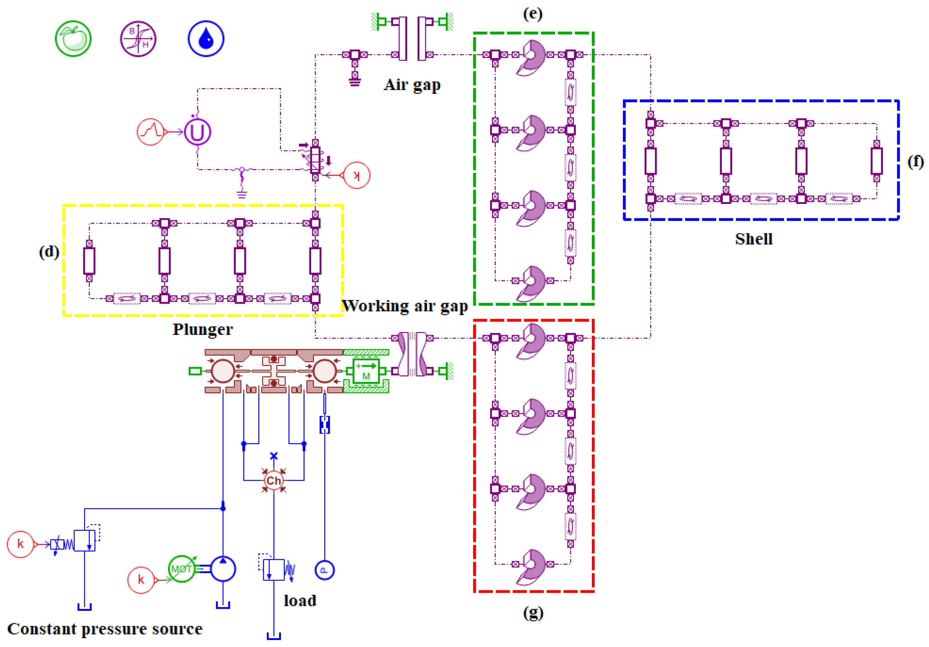
2.2. System Dynamic Modeling

The moving components of an HSV can be simplified into a second-order system. The differential equation of the movable components in the system during the opening process of the valve core can be expressed as follows:

$$M{\displaystyle \frac{d^{2}x}{d{t}^2}}+D{\displaystyle \frac{dx}{dt}}=F_e(x)+P_T{A}_s-P_a{A}_{\mathrm{s}}-F_s(x)$$

(1)

where M represents the mass of the moving components, x is the displacement of the valve core, D is the viscous damping, F_e is the output force of the electromagnetic coil as a function of the valve core displacement, P_T is the load pressure, P_a is the output pressure, and F_s is the steady-state hydraulic force function acting on the valve core when it is opening. The differential equation of the system’s moving components when the valve core is closed can be expressed as follows:

$$M{\displaystyle \frac{d^{2}x}{d{t}^2}}+D{\displaystyle \frac{dx}{dt}}=P_s{A}_s-P_a{A}_{\mathrm{s}}-F_{e2}(x)-F_{s2}(x)$$

(2)

F_e2 represents the resistance encountered when cutting magnetic field lines through the armature, and F_s2 is the steady-state hydraulic force function acting on the valve core when it is closing. By observing Equations (1) and (2), it can be understood that the valve is simultaneously affected by electromagnetic force, pressure, and hydraulic force during both opening and closing. Furthermore, these factors continuously change with the displacement of the valve core. Therefore, accurately calculating the opening and closing time requires comprehensive consideration of the mechanical, electromagnetic, and fluid effects within the system.

Magnetic force exerted by a solenoid can be mathematically represented as follows:

$$F_e={\displaystyle \frac{\phi {\left(i,x\right)}^2}{2{\mu }_0{S}_0}}$$

(3)

where S₀ is the cross-sectional area of the main air gap, and μ₀ is the vacuum permeability. The magnetic flux $\phi$ is a function of the coil current i and the position x.

$$\phi ={\displaystyle \frac{i\times n}{{\displaystyle {\sum }_{j=1}^k{R}_j}}}\times C\left(i,x\right)$$

(4)

where n is the number of turns in the coil. R_j represents the reluctance of each air gap in the magnetic path. Each reluctance can be expressed as follows:

$$R_j=L/{\mu }_{0}S$$

(5)

where S is the cross-sectional area of the magnetic path, and L is the length of the path.

Based on the calculated flux at the equivalent air gap, considering errors due to the armature’s geometric shape, core saturation, and leakage flux, the correction factor C (i, z) is calibrated using finite element analysis (FEA) results. Figure 2 compares the FEA results with the electromagnetic force model, showing that the model is accurate after calibration.

The finite element simulations of HSVs were conducted using MAXWELL 2021R1, and the results are shown in Figure 3. It can be seen that the addition of permanent magnets effectively weakens the induction intensity in most magnetic circuits, effectively avoiding the occurrence of magnetic saturation.

The voltage across the helical coil is induced by the applied power source, with its behavior being governed by the coil’s inductance, as expressed in Equation (6).The equation takes into account the resistance of the helical coil, denoted by r. Equation (6) is composed of three terms: the second term represents the back-EMF due to the coil’s self-inductance, and the third term signifies the back-EMF resulting from the helix’s motion.

$$u_i=i\cdot r+{\displaystyle \frac{\partial \phi }{\partial i}}\dot{i}+{\displaystyle \frac{\partial \phi }{\partial s}}\dot{x}$$

(6)

A model for the static hydrodynamic force acting on the valve core is established. Static hydrodynamic force refers to the force generated by the change in fluid velocity when the flow area and direction through the valve opening change, causing a change in fluid momentum. The control body, as shown in Figure 4, has a valve ball diameter of d_a, an intermediate pin diameter of d_b, and an aperture diameter of d_c at the intermediate pin location. p₁ is the inlet pressure, and p₂ is the pressure behind the valve.

Using the momentum theorem, the traditional static hydrodynamic force for a ball valve can be derived as follows:

$$F_s=\rho q\left({\beta }_2{v}_2-{\beta }_1{v}_1\right)$$

(7)

Here, F_s is the static hydrodynamic force, V₁ and V₂ are the average flow velocity vectors at the upstream and downstream flow sections, β₁ and β₂ are momentum correction coefficients, ρ is the fluid density, and q is the flow rate.

The HSV model can be expressed in the form of an equation of state shown in Equation (8).

$$\left[\begin{array}{c}{\dot{x}}_1\\ {\dot{x}}_2\\ {\dot{x}}_3\end{array}\right]=\left[\begin{array}{c}{\displaystyle \frac{\partial i}{\partial \phi \left(i,z\right)}}{u}_t-{\displaystyle \frac{\partial i}{\partial \phi \left(i,z\right)}}r{x}_1-{\displaystyle \frac{\partial i}{\partial z}}{x}_3\\ x_3\\ {\displaystyle \frac{1}{m}}\left[F_m\left(i,x_2\right)-F_s\left(\Delta P,x_2\right)-F_k\left(x_2\right)-Cu\cdot x_3\right]\end{array}\right]$$

(8)

$$y=\left[\begin{array}{ccc}1& 0& 0\end{array}\right]x$$

(9)

where the state variable represents ${\left[i,x,\dot{x}\right]}^T$.

AMESim, an acronym for an Advanced Modeling Environment for performing simulations of engineering systems, serves as a versatile platform for modeling and simulating complex multidisciplinary systems. Users can employ this unified platform to construct intricate system models encompassing various fields of study and conduct simulation calculations and in-depth analyses. Moreover, AMESim allows for the comprehensive examination of both the steady-state and dynamic performance of individual components or complete systems within the same environment [27]. It particularly excels in simulating and analyzing HSV systems. Regarding the system’s architecture, a dynamic simulation model, as depicted in Figure 5, is established. Dedicated subsystems for mechanics, hydraulics, and magnetic fields are individually developed within the system and then integrated to generate the dynamic simulation model of the HSV.

For the purpose of simplifying calculations, the dynamic simulation model of the HSV system shown in Figure 5 disregards the impact of coil temperature rise and hydraulic oil temperature during operation. The model encompasses three main systems: magnetic circuit, hydraulic, and mechanical components within the HSV. To establish a more accurate magnetic circuit model, the circuit is divided into four parts based on the simplified system model diagram, with further subdivisions based on the magnetic field distribution. The regions denoted by (d–g) in Figure 5 correspond to the respective labeled regions in Figure 6. DT4 is employed as the magnetic circuit material, and the magnetic resistances of each part can be derived from the B–H curve of the material. To emulate the real operational environment of the HSV, a quantitative pump is utilized as the fluid supply source, operating at a rotational speed of 1500 rev/min. The load is represented by a constant pressure source and an overflow valve, replicating the pressure conditions at ports A and T of the HSV during the hydraulic cylinder’s extension and retraction. The mechanical components primarily comprise the moving parts of the HSV, facilitating the simulation of valve core displacement, force status, and mass. The coupling of these three systems yields the dynamic model of the HSV.

As shown in Figure 6, where R_p is the diameter of the armature, R_t is the width of the magnetic guide ring, R_c is the thickness of the outer shell, H_t and H_b are the thickness of the upper and lower magnetic guide rings, H_s is the height of the outer shell, G₁, and G₂ are the thickness of the upper and lower nonworking air gaps, and G_w is the thickness of the working air gap. S₁ is the thickness of the pressure-resistant shell. Simulations can be performed by assigning various values to each design parameter in Figure 6a, thereby obtaining the corresponding system flow output and the currents in the coil winding. The range of values for the design parameters is presented in

Table 1. Range of values for undetermined design parameters.

	Rp (mm)	RT (mm)	Rc (mm)	Hb (mm)	Hm (mm)	Hs (mm)
Range	[3,10]	[3,6]	[3,10]	[3,10]	[5,20]	[20,50]

.

To validate the dynamic simulation model, experimental tests were performed on the valve model using the REXROTH 7920 (Bosch Rexroth, Lohr am Main, Germany). Under a 12 V power supply, the HSV valve core was actuated from the minimum to the maximum opening using three distinct duty cycle driving signals. Figure 6 illustrates the coil current measured during this process. The valve model’s simulation provides the same three distinct duty cycle driving signals, with the simulated coil current depicted in Figure 7. Due to the coil’s inductance, the current gradually increases and then stabilizes, influenced by the back electromotive force generated by the armature’s movement. When the armature contacts the valve seat, the back electromotive force diminishes, causing the coil current to continue rising rapidly. As the armature’s total displacement and mass are measured values, if the model’s coil current matches the experimental results, it demonstrates the accuracy of the modeling for inductance, back electromotive force, and valve dynamics. Figure 6 demonstrates that the current profiles for both the modeled and actual valves are essentially identical across all three duty cycles, highlighting the model’s high precision at various valve core positions. It is worth noting that in the 100% duty cycle curve after 5 ms, the measured and modeled values are different but remain unchanged. This is due to the limitation of the sensor range; according to the trend of past data, the current in the actual coil continues to increase.

3. Construction of the BPNN Model

BPNN is a multilayer feedforward neural network model known for its robust non-linear mapping and adaptive capabilities [28]. Its simple principles and structure make it particularly suitable for small datasets, minimizing the risk of overfitting. Accordingly, in this study, BPNN is employed to effectively capture the non-linear relationship between the structural parameters and performance of HSV.

The BPNN structure consists of an input layer, hidden layers, and an output layer, as illustrated in Figure 8. The input layer is composed of six neurons, corresponding to the six input structural parameters. In the output layer, there are two neurons representing the system’s output flow and the current in the winding. The hidden layers are positioned between the input and output layers. To strike a balance between training accuracy and avoiding overfitting, two hidden layers are employed. The determination of the number of neurons in the hidden layers does not have a precise formula and is often achieved using the empirical Formula (10). In the formula, H denotes the number of neurons in the hidden layers, I signifies the number of neurons in the input layer, O represents the number of neurons in the output layer, and α is a constant between 1 and 10. Activation functions are utilized to establish connections between layers, which introduce non-linear factors and augment the expressive capability of the neural network.

$$H=\sqrt{I+O}+\alpha$$

(10)

The main characteristic of BPNN is its ability to propagate signals in a forward direction and errors in a backward direction. It is a supervised learning method that relies on a training sample set with known target outputs. In the training process, the network’s weights and thresholds are initially set to random values. The signal first enters the input layer, followed by the hidden layer, and finally reaches the output layer. If the predicted values from the output layer do not match the expected outputs, error propagation occurs. The weights and thresholds of the neural network are adjusted layer by layer using the gradient descent method. As depicted in Figure 9, this adjustment process is iterative, continuing until the network’s predicted values approximate the target values and the error no longer decreases, signifying the completion of network training. Mean square error (MSE) is the most commonly used error in regression loss functions. It is the sum of the squares of the difference between the predicted value and the target value, and its formula is as follows:

$$MSE={\displaystyle \frac{{{\displaystyle \sum _{i=1}^n\left(y_i-y_i^p\right)}}^2}{n}}$$

(11)

After a comprehensive evaluation of training time and prediction accuracy through trial and error, the neural network structure is determined to be 6-12-10-2. The tansig activation function is selected for the input layer, hidden layers, and between hidden layers, while the purelin activation function is chosen between the hidden layer and the output layer. The BPNN is trained using the Levenberg–Marquardt (L–M) method, known for its fast convergence speed and low mean square error, making it suitable for training small- to medium-sized neural networks. The specific training parameters are set as follows: the learning rate is 0.0001, the maximum number of iterations is 2000, and the minimum error target for training is 0.001. The model’s accuracy is measured by the root mean square error (RMSE) and the coefficient of determination (R²), calculated using Equations (12) and (13), respectively. In these equations, $y_i$ and ${\hat{y}}_i$ represent the target and predicted values of the i-th testing sample, and ${\overline{y}}_i$ is the mean target value of the testing samples. Data normalization is performed prior to each training and testing phase, and denormalization of the network output is required. These processes facilitate the faster convergence of the network and help mitigate numerical issues.

$$RMSE=\sqrt{{\displaystyle \frac{1}{N}}{\displaystyle \sum }_{i=1}^N{(y_i-{\hat{y}}_i)}^2}$$

(12)

$$R^2=1-{\displaystyle \frac{{\displaystyle \sum _{i=1}^N{(y_i-y_i)}^2}}{{\displaystyle \sum _{i=1}^N{(y_i-{\overline{y}}_i)}^2}}}$$

(13)

The BPNN was trained and tested separately with various sample sizes, maintaining a training set to test set ratio of 7:3. The performance of the BPNN model in testing flow and current is illustrated in Figure 10. It is evident that as the sample size increases, there is a decreasing trend in the overall RMSE. At a sample size of 3000, the RMSE values for flow and current testing with the BPNN model are 0.181 and 0.223, respectively. These outcomes signify that the predictive performance of the BPNN model for flow and current improves with an increase in the sample size, thus effectively improving the effectiveness of the model fitting results.

A total of 2100 samples were selected as the training set, while 900 samples were designated for the purpose of testing the BPNN model. Figure 11 provides a visual representation of the fitting between predicted values and target values, accompanied by their respective R² values. It is evident from the figure that the BPNN model exhibits a strong linear fit for both the current (a) and flow (b) tests, with R² values approaching 1. Based on the analysis conducted, it can be concluded that the established BPNN model demonstrates a notable level of prediction accuracy, effectively capturing the nonlinear relationship between the structural parameters and performance of the HSV.

4. Utilizing AFSA for Multi-Objective Optimization Design Based on HSV

4.1. Artificial Fish Swarm Algorithm (AFSA)

The AFSA emulates the foraging behavior of fish in their natural environment. In this heuristic algorithm, artificial fish (AF) are trained independently and are able to adapt to different environments and take action on their own. Each AF can achieve four basic behaviors during training, namely following, swarm, prey, and random behavior [29]. The hunting behavior of fish can directly point to the convergence of the algorithm. Group behavior effectively enhances the robustness of algorithm convergence and ensures that it does not fall into local optima. Follow behavior effectively shortens the execution time of the algorithm and can effectively save computing resources. Random behavior constantly balances among the other three behaviors to prevent getting stuck in local optima. Each AF has two input parameters, representing the perceived visual and the step size of the movement. AF collects information and takes action through vision and steps. These behaviors of AF also tend to affect each other’s health status [30].

The AFSA draws inspiration from the behavioral characteristics of fish searching for areas with the highest food density. Here is an assumption that the state vector of an artificial fish swarm can be represented as (X = X₁, X₂, …, X_n), where X₁, X₂, …, X_n represents the corresponding positions of members in the population, and n is the total number of AFs in the calculation. The prey density is determined by the objective function Y = f (X), where the fitness function value of position X is represented by Y. In the calculation process, each AF has the ability to search for things. They can collect relevant information about food through perception, and based on this information, each AF can choose a better approach to the prey. Through communication with each other, each AF can perceive the status of other companions. AF needs to continuously move towards the target position, and the maximum distance moved each time is called the step size. In the calculation, some basic calculation parameters need to be added, including crowding factor, try_numbers, and iteration times t. Throughout the entire computation process of the AFSA algorithm, each AF can take different actions based on its current state.

Figure 12 presents the flowchart.

4.2. Objective Functions for Multi-Objective Optimization Design

Six main parameters influence the performance of the HSV. When optimizing these parameters, they are mutually constrained. Increasing the plunger diameter can enhance the operating force of the electromagnet and reduce the valve opening time. However, increasing the volume of the plunger leads to an increase in the inductance of the solenoid coil and the mass of the armature, resulting in a prolonged valve closing time. Similarly, increasing the thickness of the permanent magnet can decrease eddy current losses but may also weaken the output force of the actuator, potentially leading to a valve malfunction. The fluctuation of each parameter presents challenges in achieving an optimal solution through individual parameter optimization. The optimization design problem for a new HSV is a multi-objective optimization problem. In such problems, the sub-objectives often conflict with each other, and improving one sub-objective may compromise the performance of others. Thus, it is necessary to coordinate and compromise among sub-objectives to optimize each to the fullest extent [31]. Unlike single-objective optimization problems, multi-objective optimization problems do not have a unique solution but rather a set of Pareto optimal solutions consisting of numerous non-dominated solutions. These non-dominant solutions constitute the set of decision vectors, while the corresponding objective functions are graphically represented as the Pareto front.

Prior to performing target optimization for the ball valve, a preliminary design is conducted, where the following parameters are manually defined: ball diameter, valve seat diameter, ball valve opening, number of coil turns, and coil resistance. The parameters to be optimized in the design are R_p, R_t, R_c, H_b, H_m, and H_c. Based on the system analysis in Section 4.1, the optimization design problem for the HSV is described as follows: under given constraints, select appropriate design variables x to achieve the optimal value of the function f(x). The mathematical model is represented as follows:

$$\left\{\begin{array}{l}\min f(x)=\left\{f_{ton}(x),f_{toff}(x)\right\}\\ X_{\min }<x<X_{\max }\end{array}\right.$$

(14)

In the equation, x = (x₁, x₂, …, x₆) represents all optimization variables, which respectively represent R_p, R_t, R_c, H_b, H_m, and H_c. f(x) represents the objective function variable. x_min and x_max represent the upper bound and lower bound of the optimization variables. There are two optimization objective functions, representing the valve opening and closing times.

4.3. Optimization Results

Optimization design was conducted employing a multi-objective optimization algorithm. The individual characteristics were determined based on the structural parameters of the driving solenoid coil, and the population was initialized accordingly. Fifty randomly distributed individuals were generated within the predefined range as outlined in Table 1. The objective functions selected for this study were the opening and closing times, wherein the output flow was assessed using the established BPNN model. The opening and closing times were determined based on the valve’s output flow, with full valve opening considered achieved when the flow reached within 5% of its maximum value. The ultimate goal of the optimization process was to minimize both objective functions to the greatest extent feasible. Following the process depicted in Figure 12, iterative calculations were performed with a maximum of 200 iterations. Subsequently, all non-dominated solutions generated throughout the iterations were preserved, while duplicate non-dominated solutions were eliminated. The resulting Pareto front was visualized as a two-dimensional scatter plot. Figure 12 displays the final Pareto optimal set, consisting of 30 solutions, showcasing the opening and closing times for HSV. Each data point represents a distinct configuration of electromagnetic solenoid coil parameters, and no particular parameter configuration demonstrates superiority over others in terms of HSV’s dynamic performance. Hence, these solutions are deemed optimal.

As shown in Figure 13, the non-dominated solutions obtained through the AFSA algorithm are uniformly distributed along the Pareto front. The required opening and closing times of the ball valve are inversely proportional. This is because the proposed structure of the HSV in this study utilizes hydraulic pressure generated by the valve port differential to reset the valve core, rather than a traditional spring structure. Therefore, it is not possible to adjust the reset force by modifying the spring stiffness or precompression. Additionally, the model developed in this study considers the influence of eddy current losses on response time. The reset time of the valve is greatly affected by the inductance of the driving solenoid coil. While increasing the driving force of the electromagnet, the inductance and eddy current losses also increase, resulting in an inability to simultaneously decrease the opening and closing times of the electromagnet.

5. Prototype and Experiment

To validate the performance of the proposed HSV, a prototype was fabricated based on the computation results obtained from the AFSA algorithm. The prototype, denoted as HSV, is illustrated in Figure 13. As it is not feasible to directly measure the valve core opening, its movement can be observed by monitoring the input current to the solenoid coil and the flow rate. A test setup, as depicted in Figure 14, was devised specifically for this purpose. Since the flow channels from port P to port A and from port T to port A in the HSV are identical, it sufficed to test only one of them. The hydraulic pump was configured to generate an output pressure of 14 MPa, and this pressurized fluid was directed through the HSV before being measured by a flow meter. The flow meter provided a signal that was recorded by a data acquisition device, while the flowing hydraulic fluid subsequently entered the relief valve, which served to simulate the load. Following the relief valve, the fluid was channeled into the oil tank. The HSV was actuated by a step signal produced by a signal generator, with the current output from the flow transmitter and the pressure transmitter being captured by an oscilloscope. A step signal, lasting 50 ms and possessing a voltage of 12 V, was applied as an input to the HSV system, with the resulting current and flow data being recorded.

Table 2. Design parameters to be determined.

Item	Model	Range	Remarks
Signal generator	OHR-B00	1–10 kHz (±100 Hz)
Pump	-	0–30 mPa	Max 50 L/min
Flow probe	KRACHT TM8 TFC250S	0–8 L/min	25 °C
Pressure probe	AR-SS-SZJ06	0.1~14.0 mPa
Relief valve	DBET-6X/315G24K4 V	0.1~31.5 mPa	Max 10 L/min

shows the model and parameters of the equipment used in the experiment, while

Table 3. Optimization results.

	Rp (mm)	RT (mm)	Rc (mm)	Hb (mm)	Hm (mm)	Hs (mm)
Initial	4.6	4.55	3.2	3.6	~	36.4
Optimal	5.3	4.2	4.1	5.5	6.5	43.1

displays the initial and optimized dimensions of the valve.

The experimental results depicted in Figure 14 provide insights into the displacement behavior of the ball valve through the analysis of recorded currents. When the step control signal was applied, the solenoid coil experienced inductance that impeded the increase in coil current. Insufficient input current prevented the armature from overcoming the pre-tightening force of the spring, resulting in an initial rise in current with no armature displacement. In the subsequent stage, the armature began to displace. The motion of the armature induced a back electromotive force due to the cutting of the magnetic flux lines, causing the driving current to decrease. However, the valve core quickly stopped and the driving current continued to rise until it reached its maximum value. Similarly, the closing process of the solenoid valve can be divided into two parts. After the control voltage rapidly dropped to zero, the armature could not move due to the interaction between coil eddy currents, inductance, and residual magnetic fields of the rotor. As the current decreased, the force generated could not continue to attract the armature. Under the action of the reset spring, the armature was pushed out until the maximum air gap was reached. The opening action of the valve core took about 3 ms, and the closing action took about 3 ms.

The black dashed line in Figure 15 represents the BPNN’s fitted output for the design parameter. By examining the flow output curve of the HSV, it becomes evident that, apart from a significant deviation at the initial movement of the valve and around its maximum opening, the predicted flow output and opening time of the HSV closely align with the experimental results. An analysis of the predicted current variation in the solenoid coil indicated that the BPNN exhibits some error in predicting the armature movement and the maintenance current; however, the overall trend remains consistent. In conclusion, the BPNN, trained using the system dynamics simulation model, demonstrates a substantial capability to accurately predict the system output.

Valves in hydraulic systems introduce resistance to the passage of fluid. This resistance grows as the flow rate increases. Consequently, the flow–pressure curve, also referred to as the P–Q curve, holds significant importance in fluid systems. By conducting experiments to adjust the output flow rate of the quantitative pump and analyzing the pressure data both upstream and downstream of the HSV, it is possible to construct the flow–pressure drop curve for the HSV (Figure 16). It is evident that as the pressure drop rises, the output flow rate of the HSV steadily increases, peaking at a pressure drop of 7 MPa, approximately equal to 1 L/min.

6. Conclusions

This paper proposes a multi-objective optimization approach that integrates neural networks with the AFSA algorithm to achieve high-fidelity modeling and an efficient optimization design of high-speed on/off valves. Starting from simplifying mathematical modeling, using neural networks to replace traditional modeling not only saves computational resources but also ensures the accuracy of modeling. By establishing a BPNN model to capture the nonlinear relationship between structural parameters and performance, the need for approximating the valve’s open and close processes using functions is eliminated. Following training and testing, the BPNN model demonstrates low RMSE and high R² values. Employing this BPNN model in conjunction with the AFSA algorithm yields a Pareto optimal solution set comprising 30 solutions, allowing for the selection of optimal design parameters. To evaluate the response speed of the high-speed on/off valve, a prototype was manufactured and a dedicated experimental platform was constructed, revealing an opening time and closing time of 3 ms for the designed structure. Comparing the experimental results with the predicted outputs of the trained backpropagation neural network further attests to the network’s precise predictions, thereby reinforcing the viability of the proposed system modeling approach. The method proposed in this article is not only of great significance for the structural optimization design of high-speed on/off valves but also has more experimental data training. It will have a wider range of applications in the fault detection of various types of valves in hydraulic systems and the field of digital twins.

References

1. Fei, J.; Wu, Z.; Sun, X.; Su, D.; Bao, X. Research on tunnel engineering monitoring technology based on BPNN neural network and MARS machine learning regression algorithm. Neural Comput. Appl. 2021, 33, 239–255. [Google Scholar] [CrossRef]
2. Laamanen, M.S.A.; Vilenius, M. Is it time for digital hydraulics. In Proceedings of the Eighth Scandinavian International Conference on Fluid Power, Tampere, Finland, 7–9 May 2003. [Google Scholar]
3. Wang, S.; Zhang, B.; Zhong, Q.; Yang, H. Study on control performance of pilot high-speed switching valve. Adv. Mech. Eng. 2017, 9, 1687814017708908. [Google Scholar] [CrossRef]
4. Zhang, Q.; Kong, X.; Yu, B.; Ba, K.; Jin, Z.; Kang, Y. Review and development trend of digital hydraulic technology. Appl. Sci. 2020, 10, 579. [Google Scholar] [CrossRef]
5. Azzam, I.; Pate, K.; Garcia-Bravo, J.; Breidi, F. Energy savings in hydraulic hybrid transmissions through digital hydraulics technology. Energies 2022, 15, 1348. [Google Scholar] [CrossRef]
6. Zhong, Q.; Li, X.; Mao, Y.; Xu, E.; Jia, T.; Li, Y.; Yang, H. Switching Frequency Improvement of a High Speed on/off Valve Based on Pre-excitation Control Algorithm. Chin. J. Mech. Eng. 2024, 37, 88. [Google Scholar] [CrossRef]
7. Yue, D.; Li, L.; Wei, L.; Liu, Z.; Liu, C.; Zuo, X. Effects of pulse voltage duration on open–close dynamic characteristics of solenoid screw-In cartridge valves. Processes 2021, 9, 1722. [Google Scholar] [CrossRef]
8. Zhang, B.; Zhong, Q.; Ma, J.E.; Hong, H.C.; Bao, H.M.; Shi, Y.; Yang, H.Y. Self-correcting PWM control for dynamic performance preservation in high speed on/off valve. Mechatronics 2018, 55, 141–150. [Google Scholar] [CrossRef]
9. Wang, X.J.; Li, W.J.; Li, C.H.; Peng, Y.W. Structure optimization and flow field simulation of plate type high speed on-off valve. J. Cent. South Univ. 2020, 27, 1557–1571. [Google Scholar] [CrossRef]
10. Yang, H.; Wang, W.; Lu, K.; Chen, Z. Cavitation reduction of a flapper-nozzle pilot valve using continuous microjets. Int. J. Heat Mass Transf. 2019, 133, 1099–1109. [Google Scholar] [CrossRef]
11. Feng, Y.; Xu, T.; Dai, Y. Dynamic optimization method of High-speed solenoid valve parameters. J. Phys. Conf. Ser. 2022, 2296, 012001. [Google Scholar] [CrossRef]
12. Yang, S.; Yao, J.; Wang, P.; Zhang, P.; Wei, T.; Li, D. A novel Dual-Magnetic circuit actuated Fast-Switching valve with Multi-Stage excitation control algorithm. Measurement 2024, 230, 114483. [Google Scholar] [CrossRef]
13. Chu, Y.; Yuan, Z.; Chang, W. Research on the dynamic erosion wear characteristics of a nozzle flapper pressure servo valve used in aircraft brake system. Math. Probl. Eng. 2020, 2020, 3136412. [Google Scholar] [CrossRef]
14. Qingtong, L.; Fanglong, Y.; Songlin, N.; Ruidong, H.; Hui, J. Multi-objective optimization of high-speed on-off valve based on surrogate model for water hydraulic manipulators. Fusion Eng. Des. 2021, 173, 112949. [Google Scholar] [CrossRef]
15. Madsen, E.L.; Jørgensen, J.M.; Nørgård, C.; Bech, M.M. Design optimization of moving magnet actuated valves for digital displacement machines. In Fluid Power Systems Technology; American Society of Mechanical Engineers: New York, NY, USA, 2017; Volume 58332, p. V001T01A026. [Google Scholar]
16. Abdel-Basset, M.; Abdel-Fatah, L.; Sangaiah, A.K. Metaheuristic algorithms: A comprehensive review. In Computational Intelligence for Multimedia Big Data on the Cloud with Engineering Applications; Elsevier: New York, NY, USA, 2018; pp. 185–231. [Google Scholar]
17. Zhong, C.; Li, G.; Meng, Z. Beluga whale optimization: A novel nature-inspired metaheuristic algorithm. Knowl.-Based Syst. 2022, 251, 109215. [Google Scholar] [CrossRef]
18. Zhao, W.; Wang, L.; Zhang, Z.; Fan, H.; Zhang, J.; Mirjalili, S.; Cao, Q. Electric eel foraging optimization: A new bio-inspired optimizer for engineering applications. Expert Syst. Appl. 2023, 238, 122200. [Google Scholar] [CrossRef]
19. Wei, J.; Ju, Y. Research on optimization method for traffic signal control at intersections in smart cities based on adaptive artificial fish swarm algorithm. Heliyon 2024, 10, e30657. [Google Scholar] [CrossRef]
20. Yuan, M.; Kan, X.; Chi, C.; Cao, L.; Shu, H.; Fan, Y. An adaptive simulated annealing and artificial fish swarm algorithm for the optimization of multi-depot express delivery vehicle routing. Intell. Data Anal. 2022, 26, 239–256. [Google Scholar] [CrossRef]
21. Tang, Q.; Wu, R.; Ji, J.; Liu, J.; Li, Z. Research on illumination optimization of phototherapy LED based on multi-objective artificial fish swarm algorithm. J. Appl. Opt. 2021, 42, 352–359. [Google Scholar]
22. Ma, C.; He, R. Green wave traffic control system optimization based on adaptive genetic-artificial fish swarm algorithm. Neural Comput. Appl. 2019, 31, 2073–2083. [Google Scholar] [CrossRef]
23. Wu, S.; Zhao, X.; Li, C.; Jiao, Z.; Qu, F. Multiobjective optimization of a hollow plunger type solenoid for high speed on/off valve. IEEE Trans. Ind. Electron. 2017, 65, 3115–3124. [Google Scholar] [CrossRef]
24. Li, T.; Zhang, Y.; Liang, Y.; Yang, Y.; Jiao, J. Multiobjective optimization research on the response time of a pneumatic pilot-operated high speed on/off valve. Int. J. Appl. Electromagn. Mech. 2021, 65, 109–127. [Google Scholar] [CrossRef]
25. Kassaymeh, S.; Al-Laham, M.; Al-Betar, M.A.; Alweshah, M.; Abdullah, S.; Makhadmeh, S.N. Backpropagation Neural Network optimization and software defect estimation modelling using a hybrid Salp Swarm optimizer-based Simulated Annealing Algorithm. Knowl.-Based Syst. 2022, 244, 108511. [Google Scholar] [CrossRef]
26. Li, P.; Zhang, Y. Influence of eddy current on transient characteristics of common rail injector solenoid valve. J. Beijing Inst. Technol. 2015, 24, 26–34. [Google Scholar]
27. Wan, L.; Yu, X.; Zeng, X.; Ma, D.; Wang, J.; Meng, Z.; Zhang, H. Performance analysis of the new balance jack of anti-impact ground pressure hydraulic support. Alex. Eng. J. 2023, 62, 157–167. [Google Scholar] [CrossRef]
28. Hannan, M.A.; Lipu, M.S.H.; Hussain, A.; Saad, M.H.; Ayob, A. Neural network approach for estimating state of charge of lithium-ion battery using backtracking search algorithm. IEEE Access 2018, 6, 10069–10079. [Google Scholar] [CrossRef]
29. Pourpanah, F.; Wang, R.; Lim, C.P.; Wang, X.Z.; Yazdani, D. A review of artificial fish swarm algorithms: Recent advances and applications. Artif. Intell. Rev. 2023, 56, 1867–1903. [Google Scholar] [CrossRef]
30. Zhang, H.; Hong, Q.; Shi, X.; He, J. A social tagging recommendation model based on improved artificial fish swarm algorithm and tensor decomposition. In Security with Intelligent Computing and Big-data Services; Springer International Publishing: Cham, Switzerland, 2018; pp. 3–13. [Google Scholar]
31. Li, X.L. An optimizing method based on autonomous animats: Fish-swarm algorithm. Syst. Eng.-Theory Pract. 2002, 22, 32–38. [Google Scholar]
Figure 1. Schematic diagram of the structure of the new HSV.
Applsci 14 07879 g001
Figure 2. Validation of the electromagnetic force model.
Applsci 14 07879 g002
Figure 3. FEA simulation schematic diagram.
Applsci 14 07879 g003
Figure 4. Static hydrodynamic force calculation diagram.
Applsci 14 07879 g004
Figure 5. Dynamic simulation model of the system. The three symbols in the upper left corner represent the gravity, electromagnetic, and oil properties in the simulation.
Applsci 14 07879 g005
Figure 6. (a) Simplified diagram of the system model, (b) Illustration of magnetic circuit division.
Applsci 14 07879 g006
Figure 7. Experimented coil current for validation of the valve model.
Applsci 14 07879 g007
Figure 8. Schematic diagram of BPNN structure.
Applsci 14 07879 g008
Figure 9. Training error of the network.
Applsci 14 07879 g009
Figure 10. Train the BPNN model with different sample sizes and test its performance on Gain and NF.
Applsci 14 07879 g010
Figure 11. The fitting between the predicted values and target values of the BPNN model.
Applsci 14 07879 g011
Figure 12. Flowchart of the HSV-optimized AFSA algorithm based on BPNN.
Applsci 14 07879 g012
Figure 13. Distribution of multi-objective optimization solution set.
Applsci 14 07879 g013
Figure 14. Schematic diagram of the hydraulic circuit in the experimental system.
Applsci 14 07879 g014
Figure 15. The process of system opening and closing.
Applsci 14 07879 g015
Figure 16. Flow-pressure drop curve.
Applsci 14 07879 g016