Featured Application
(1) The concept of trip assignment probability was used to simulate passenger behavior of selecting different HSR stations in a zone, unlike the existing all-or-nothing-based optimal strategy algorithm. (2) By optimizing the trip assignment probability using a backpropagation-based algorithm, the accuracy and time efficiency of long-term HSR demand forecasting were improved compared with the existing calibration process using a trial-and-error approach. (3) The estimation accuracy of the backpropagation-based algorithm was especially superior when applied to an area with multiple accessible HSR stations, such as the Seoul metropolitan area, as well as non-metropolitan areas with a single accessible HSR station.
Abstract
In Korea, decisions for high-speed railway (HSR) construction are made based on long-term demand forecasting. A calibration process that simulates current trip patterns is an important step in long-term demand forecasting. However, a trial-and-error approach based on iterative parameter adjustment is used for calibration, resulting in time inefficiency. In addition, the all-or-nothing-based optimal strategy algorithm (OSA) used in HSR trip assignment has limited accuracy because it assigns all trips from a zone with multiple accessible stations to only one station. Therefore, this study aimed to develop a backpropagation-based algorithm to optimize trip assignment probability from a zone to multiple accessible HSR stations. In this algorithm, the difference between the estimated volume calculated from the trip assignment probability and observed volumes was defined as loss, and the trip assignment probability was optimized by repeatedly updating in the direction of the reduced loss. The error rate of the backpropagation-based algorithm was compared with that of the OSA using KTDB data; the backpropagation-based algorithm had lower errors than the OSA for most major HSR stations. It was especially superior when applied to areas with multiple HSR stations, such as the Seoul metropolitan area. This algorithm will improve the accuracy and time efficiency of long-term HSR demand forecasting.
1. Introduction
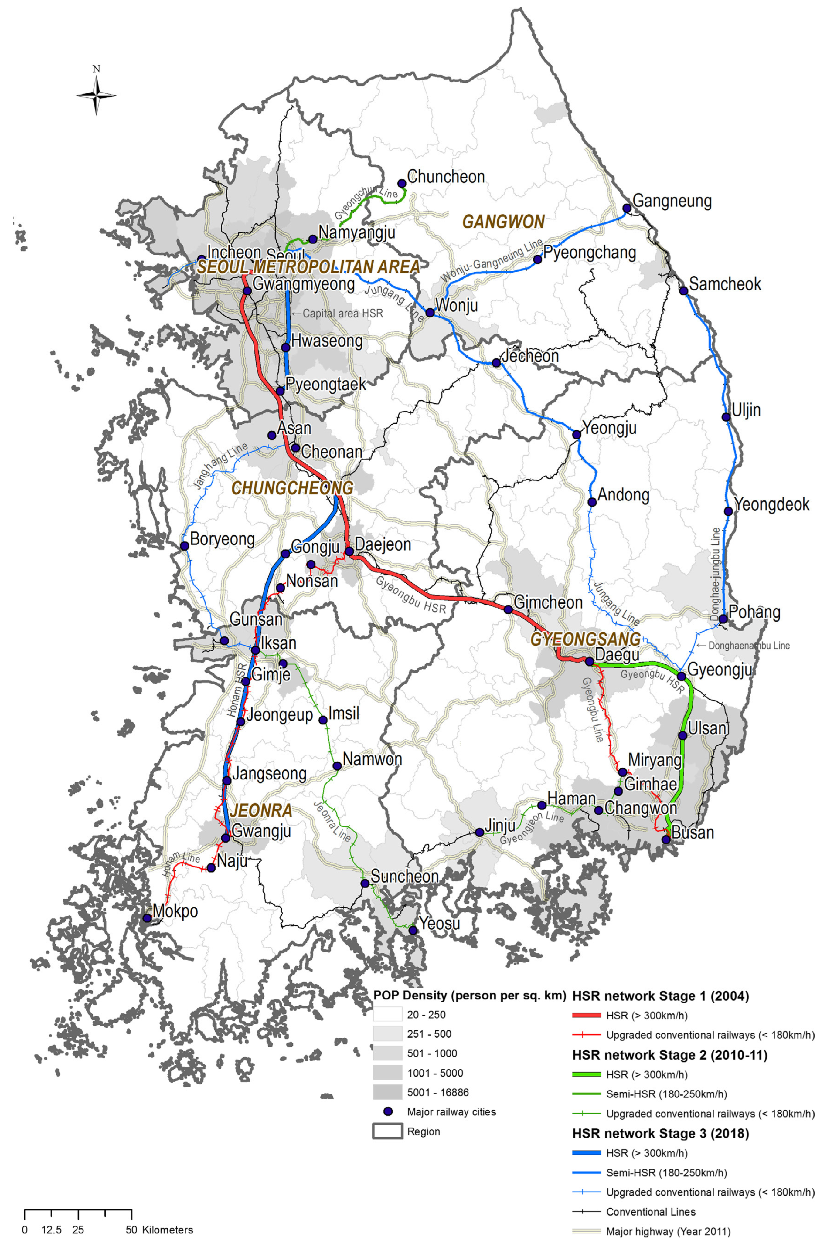
High-speed railway (HSR) networks are significantly expanding on a global level. The length of HSRs was about 44,000 km in 2017, increasing by more than 30% to about 59,000 km in 2022 [1]. The HSR network in Korea has also expanded to about 893 km since it opened in 2004, as shown in Figure 1 [2], and the number of passengers has increased from 37,394 thousand persons in 2009 to 89,420 thousand persons in 2019 [3]. HSRs are used for operations of at least 250 km/h by UIC [4], but in Korea they have a maximum speed of over 300 km/h. In response to increasing demand, projects to build several HSR lines have been undertaken by the Korean Government. The impacts of these projects need to be evaluated using preliminary feasibility studies to secure part of the national budget, and the impacts are quantified based on long-term demand-forecasting results.
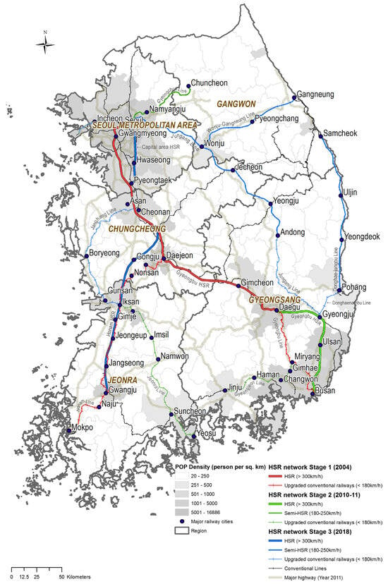
Figure 1.
The HSR network in Korea [2].
The standard procedure for long-term demand forecasting in preliminary feasibility studies is included in a guideline published by the Korea Development Institute, which is a national research institute [5]. According to the guideline, the long-term demand for HSR is predicted based on the premise that the current trip patterns will be maintained in the future. Therefore, the calibration process to simulate the current trip patterns is one of the most important steps in the long-term demand forecasting procedure. However, the guideline does not provide a specific methodology for calibration; therefore, analysts apply a trial-and-error approach to correct the error between the observed volume and estimated volume using a trip assignment model. This approach causes a large amount of time loss in long-term demand-forecasting analysis. Therefore, it is necessary to develop a time-efficient long-term demand-forecasting algorithm.
A variety of machine learning (ML)-related algorithms have been used to improve accuracy and time efficiency. In railway demand forecasting, ML is mainly focused on short-term forecasting. Short-term demand forecasting estimates the daily/hourly demand and establishes train operation plans. It aims to improve service quality and to reduce operating costs by adjusting operation plans. The most recent research on short-term passenger flow prediction has used the long short-term memory (LSTM)-based model or a combined model to capture the spatiotemporal features of historical passenger flow data in Chinese urban railway networks [6,7,8,9,10,11,12,13,14,15,16]. Han et al. proposed a novel deep-learning-based passenger flow (inflow and outflow) volume prediction approach using graph convolutional neural networks to capture spatiotemporal dependencies [17]. Hao et al. proposed a sequence-to-sequence model with an embedded attention mechanism to predict the alighting passenger volume at each Singapore metro station in the near future given the boarding passenger volume at each station in the last few short-term periods [18]. Wang et al. predicted the weekly periodicity and nonlinearity characteristics of short-term (5 min) ridership using a support vector machine (SVM) combined online model at two stations of the Nanjing Metro [19]. Roos et al. forecasted short-term passenger flows in the urban rail network of Paris with incomplete data based on dynamic Bayesian networks [20]. Sun et al. proposed a novel hybrid model Wavelet-SVM to predict different kinds of passenger flows (high frequency and low frequency) in the Beijing subway [21]. Wei and Chen developed a hybrid EMD-BPN forecasting approach that combines empirical mode decomposition (EMD) and backpropagation neural networks (BPNs) to predict short-term passenger flow in Taipei’s rapid transit [22]. In addition, several research works have predicted abnormal or irregular congested passenger flow [23,24,25,26], and a few scholars have established models to predict short-term HSR demand. Zhao and Mi proposed a hybrid model that predicts short-term demand for an HSR by combining singular spectrum analysis, a convolutional neural network (CNN), and support vector regression [27]. Jiang et al. developed a hybrid approach combining the ensemble empirical mode decomposition (EEMD) and gray support vector machine (GSVM) for the short-term prediction of HSR flows [28]. When planning and constructing a new railway line or station, the influencing factors of demand become the variables for long-term demand forecasting. Du et al. proposed several factors affecting long-term passenger flow in rail transit, constructing a prediction model based on a class neural network [29]. Lin et al. focused on investigating the relationship between the built environment around the station and its passenger flow, developing a passenger flow prediction model using a multilayer perceptron (MLP) that could be applied to new railway stations without historical passenger flow data [30]. Lin et al. used mathematical and neural network methods to predict metro passenger flow based on land use around stations [31]. Yu et al. divided a city into multiple regions with similar internal traffic properties and a moderate spatial size to obtain more accurate factors affecting passenger flow, proposing a new prediction model based on the fuzzy processing method and Xgboost [32]. He et al. proposed a passenger flow prediction model based on station attributes affecting passenger flow regularity and predicted the passenger flow of a new line or station using its own attributes [33]. Cao et al. presented a new system with deterministic and probabilistic forecasting capacities based on residual component disposing for HSR demand forecasting [34]. Using long-distance elasticities, Börjesson investigated the prediction performance of two state-of-the-art Swedish HSR demand-forecasting models: the nested logit-based Sampers long-distance model and the newly developed Box-Cox transformation-based model [35]. Thus, a large number of researchers are engaged in this topic on all continents.
The optimal strategy algorithm has been widely used not only academically but also practically in railway trip assignment models [36,37]. This algorithm assigns origin–destination (O/D) trips to the route that minimizes passenger travel time among various route options. The procedure is as follows [38]:
- Define a departure node (station or stop);
- Move to and board the vehicle that arrives first at the departure node among the competing routes;
- Get off at the intermediate node (station or stop) that was determined according to the optimal strategy;
- End if the passenger arrives at their destination; otherwise, define the alighting node as the departure node and repeat from step 1.
This approach is limited when simulating access trip patterns from each zone to diverse railway stations because this algorithm is based on an all-or-nothing trip assignment approach assigning all trips to only one railway station that minimizes the generalized cost. Tavassoli et al. proposed a practical procedure that automatically calibrates and validates large-scale transit assignments based on the optimal strategy [36]. They used smart card data and adopted a particle swarm optimization (PSO) algorithm as an optimization technique. De Cea and Fernandez [39] and Wu et al. [40] improved the optimal strategy algorithm to simulate congestion and delay by considering capacity constraints in the optimal strategy, but they did not overcome other limitations.
There are many access modes to HSR stations, and those selected by passengers will vary depending on the preferred access modes in a zone. Furthermore, in an HSR trip, the proportion of access time compared with in-vehicle time in the total travel time is higher than that of other public transportation. Therefore, it is necessary to develop a trip assignment algorithm that can reflect the diverse passenger preferences for accessibility to HSR stations.
In this study, we developed a backpropagation-based algorithm to optimize trip assignment probability from each zone to accessible HSR stations. This improves the accuracy and time efficiency of long-term HSR demand forecasting by reflecting the various access patterns of HSR passengers and using an optimization-based calibration algorithm.
The remainder of this paper is organized as follows: Section 2 reviews the standard long-term HSR demand forecasting methodology in Korea. Section 3 explains the trip assignment probability and optimizing algorithm for HSRs. Section 4 describes the data used and discusses the case study results. Section 5 presents conclusions and ideas for future research.
2. Standard Long-Term HSR Demand-Forecasting Methodology in Korea
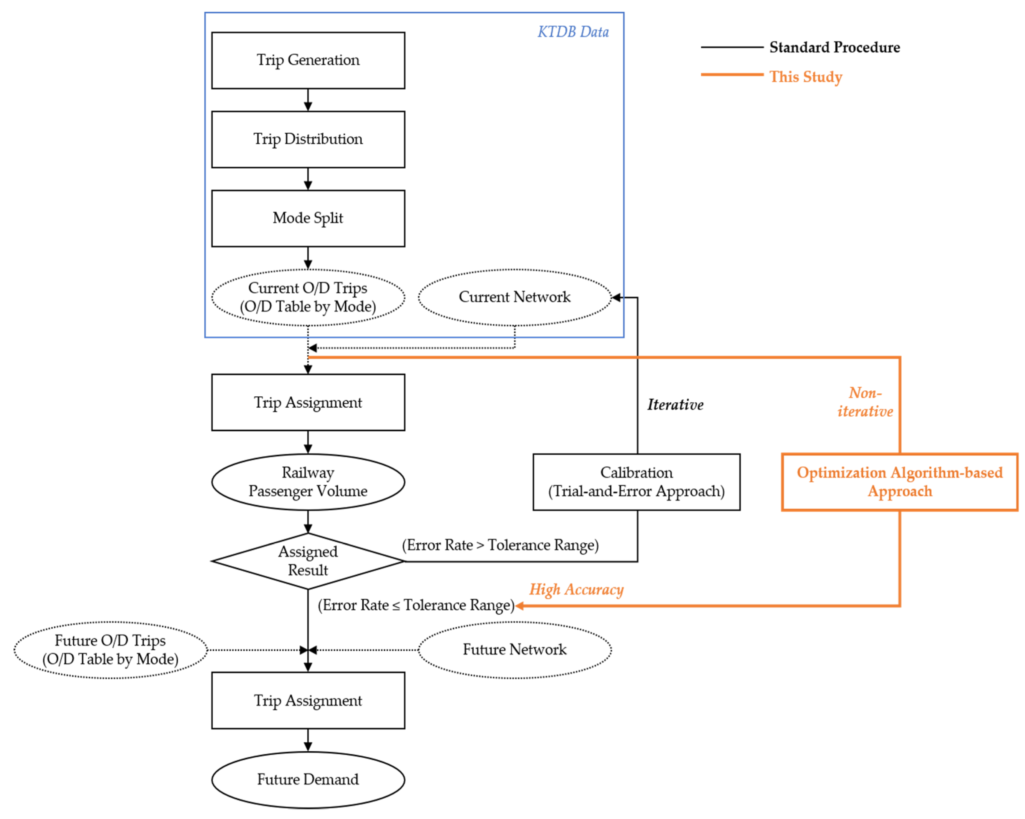
This section introduces the standard long-term HSR demand-forecasting method in Korea. A preliminary feasibility study is a system in which government agencies review the feasibility of a project in advance. A preliminary feasibility study must be conducted for projects costing USD 35 million (KRW 50 billion) or more. The guideline for a preliminary feasibility study presents a long-term demand-forecasting methodology. The guideline provides a conventional four-step method of trip generation, trip distribution, mode split, and trip assignment for long-term demand forecasting, as shown in Figure 2 [5]. The O/D trip and network data included in the Korea Transport Database (KTDB) are used in this process. Since the KTDB includes O/D data by mode, the first three steps (trip generation, trip distribution, and mode split) in the conventional four-step method are omitted when predicting long-term demand. Therefore, the accuracy of the long-term demand forecasting varies according to the trip assignment algorithm. An optimal strategy algorithm without capacity constraints is applied for long-term railway demand forecasting using macrosimulations, such as Emme or TransCAD. To simulate the current trip pattern of a trip assignment algorithm, a calibration process based on a trial-and-error approach is iteratively performed to correct the error between the volume estimated by the algorithm and the observed volume. After the calibration process, the long-term demand is predicted by applying the calibration results to the future network.
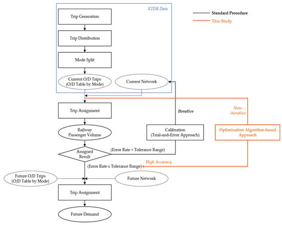
Figure 2.
Standard long-term HSR demand-forecasting procedure in Korea.
The calibration reference value in railway trip assignment is the error rate between the estimated and observed boarding/alighting volumes at major stations, calculated as Equation (1) [5]. The guideline suggests that the error rate must be under 30% for stations but does not provide specific calibration methods. Accordingly, the analyst repeats the calibration process, such as by adjusting the network parameter, to satisfy the 30% critical error rate; however, there are limits to improving this accuracy due to the temporal inefficiency and limitations of the all-or-nothing-based optimal strategy algorithm:
where is the estimated number of passengers at each station using the trip assignment model, and is the observed number of passengers at each station.
3. Methods
3.1. Trip Assignment Probability
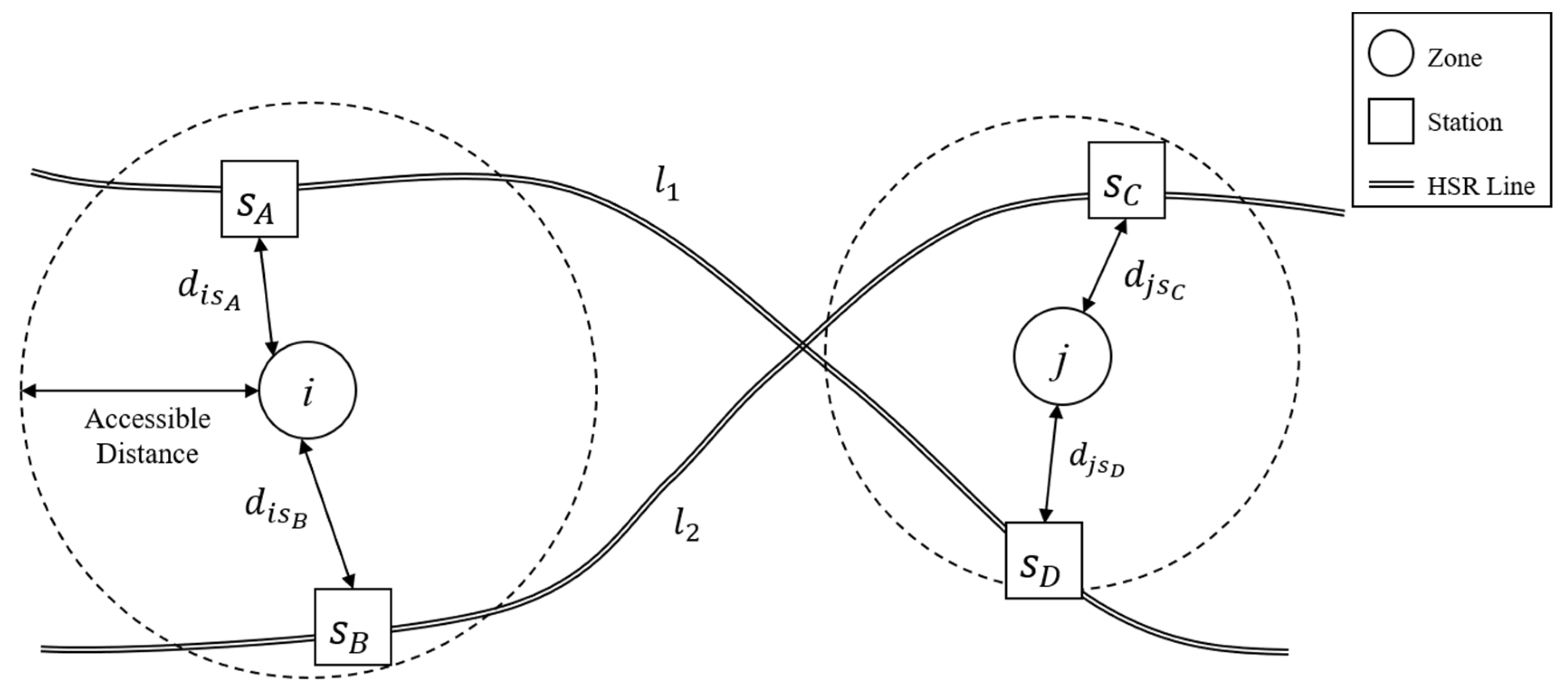
The trip assignment probability is calculated by extracting the accessible HSR stations for each zone by route. The trip assignment probability concept is shown in Figure 3. Unlike the optimal strategy algorithm, this method can simulate the passenger behavior of selecting different HSR stations in a zone. For zone i, stations and within the accessible distance are considered accessible stations, and station is excluded because it is outside the accessible distance. Thus, the HSR trips from zone i are assigned to and . The passengers are assigned in the same way for the departure and arrival zones. If the departure and arrival stations are on the same line, then X = 1; otherwise, X = 0, and the passenger volume between the two stations equals zero. For example, in Figure 3, , but . The inter-station passenger volume, , is equal to the sum of all stations multiplied by , the probability of using station in zone i; , the probability of using station in zone j; and , the O/D trips from zone i to zone j. If and are not connected on the same line (), becomes 0.
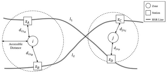
Figure 3.
The trip assignment probability concept.
Passengers can access different stations, even within the same zone, based on impedances experienced in traveling to the station or the service level of the station. Yao and Morikawa found that induced demand increases with decreased travel time, travel costs, and access time, and increased service frequency [41]. Choi et al. used walking distance to the station as an influential factor for metro ridership [42]. Moreover, the vehicle frequency of public transportation is the most crucial factor of the trip assignment in the optimal strategy algorithm [38]. Therefore, we considered , the Euclidean distance from zone i to station s, to be a travel impedance factor, and , the train frequency at station s, to be a travel attractiveness factor.
3.2. Optimization Algorithm
The HSR trip assignment model outputs the predicted demand for each station when influencing factors are input. An artificial neural network algorithm that has recently been used in many ways owing to its high prediction performance could be applied to this problem. This algorithm learns the relationship between inputs and outputs based on collected data and then highly accurately outputs the results by optimizing the weight using a backpropagation algorithm [43]. The backpropagation algorithm optimizes the weight to minimize loss, which is the error margin between a prediction and the actual target value. After a gradient is obtained for each weight, the weight is updated in the opposite (negative) direction. In this study, we used the trip assignment probability concept, but the probability could not be used as an output in the modeling because of limitations in data acquisition. When we applied backpropagation to this problem, the trip assignment probability could be recognized as the weight optimized in the artificial neural network. In other words, it could be approached as an optimization problem: finding a trip assignment probability that minimizes loss, that is, the difference between the estimated volume based on this probability and the observed volume. Therefore, the trip assignment probability was estimated using an optimization technique based on backpropagation.
In addition, considering that accessible stations may vary depending on the line, the trip assignment probability was estimated using a combination of zones and lines, not just zones. We assumed that there were n accessible stations for each combination of zones and lines; thus, n probabilities for each combination were estimated using the optimization algorithm. If there were N combinations and n accessible stations for each combination, (N × n) probabilities needed to be estimated. The sum of the probabilities for n accessible stations is 1. The trips provided as a combination of zones and lines were assigned to each accessible station, along with their probabilities, and the assigned trips were added up for each station to calculate the boarding/alighting volume at each station.
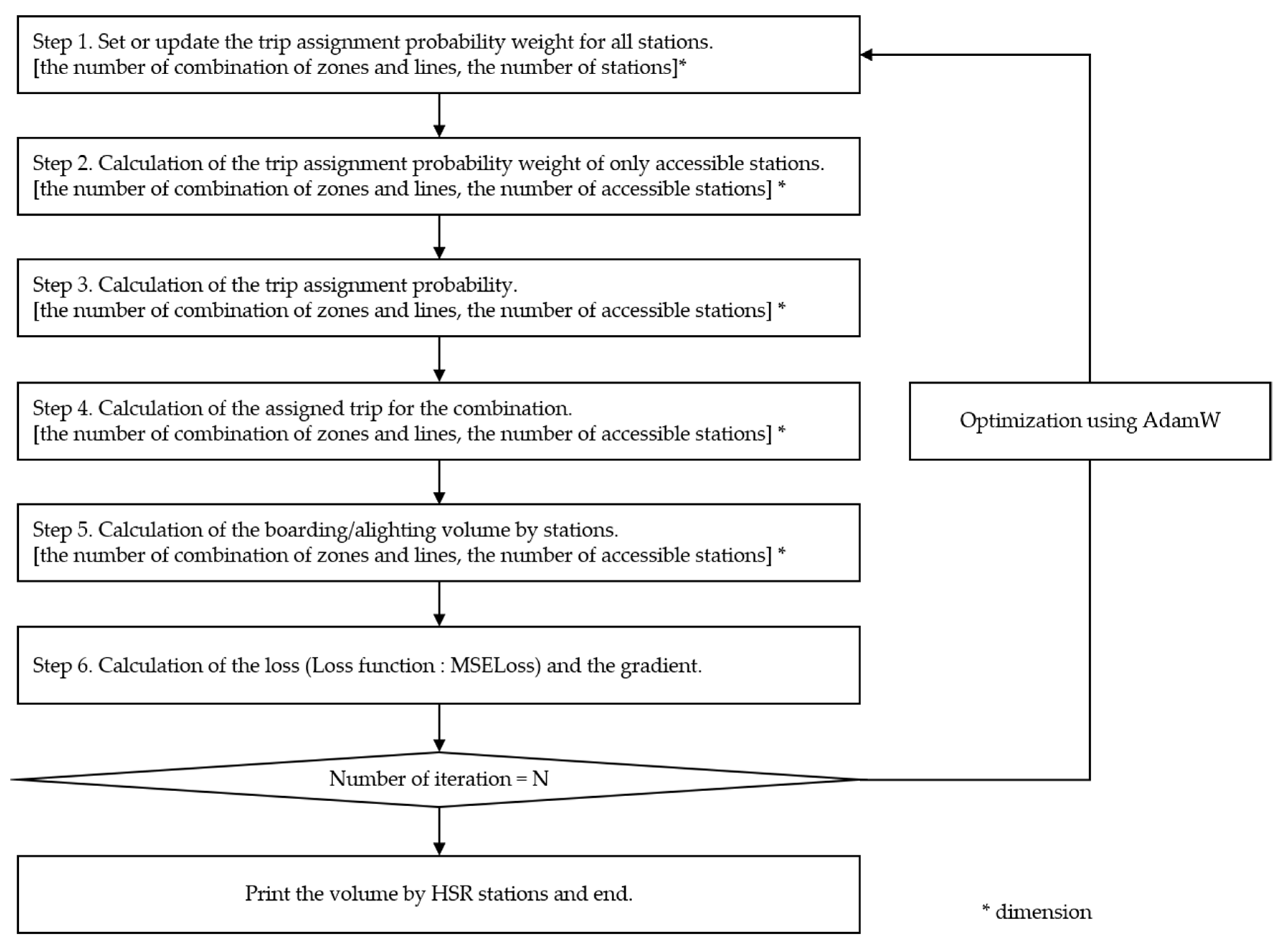
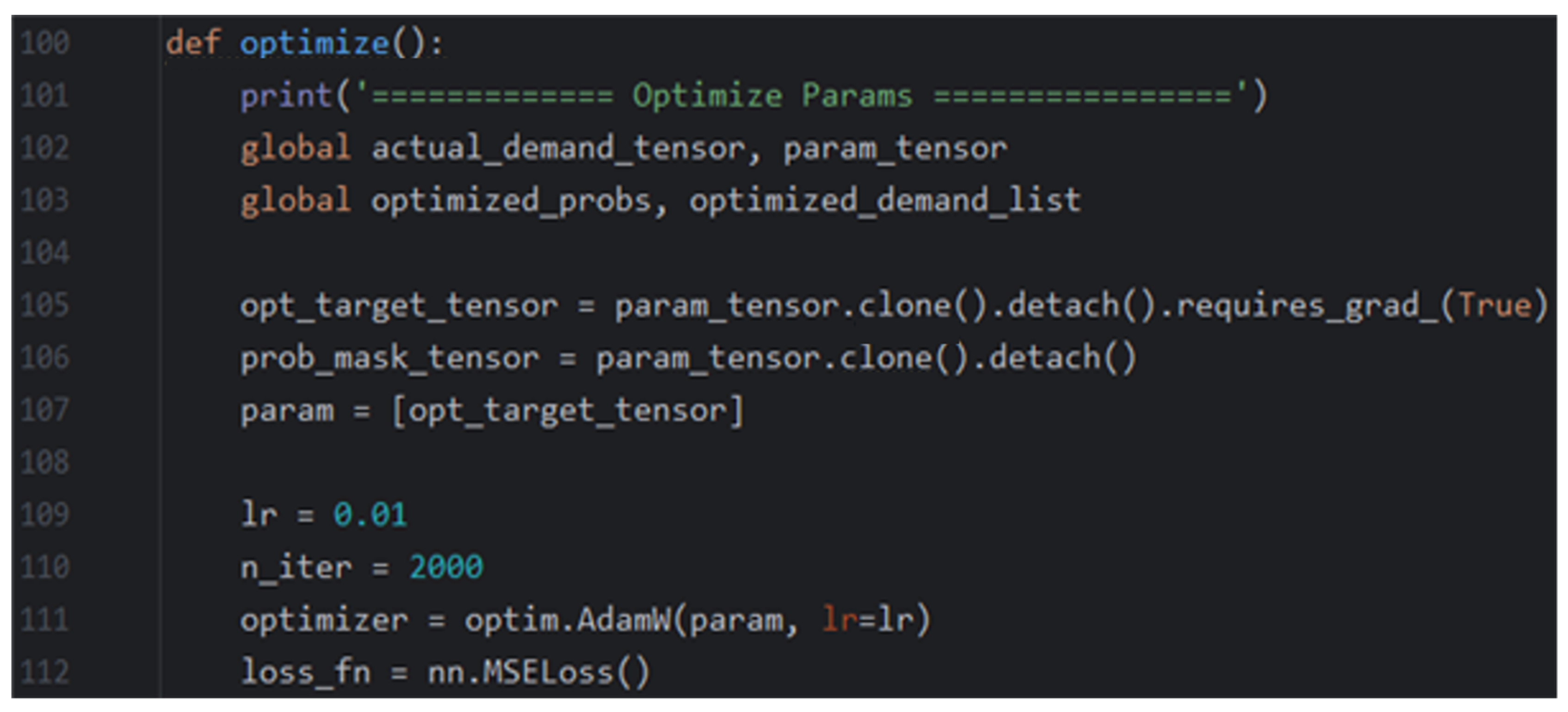
However, to apply this backpropagation concept, the loss calculation process must be differentiable. In this study, PyTorch 1.11 [44] was used, a deep learning framework used for artificial neural network learning, and it provided the loss value using only differentiable calculations. Backpropagation is the basic principle for weight updates, and several optimization algorithms exist depending on how backpropagation is applied. In this study, the AdamW algorithm [45] was applied as the optimization algorithm, and MSELoss (mean squared error loss) was used as the loss function as shown in Figure A1. The procedure is shown in Figure 4, and its detailed codes are presented in Figure A2 for readers to better analyze and repeat the experiment.
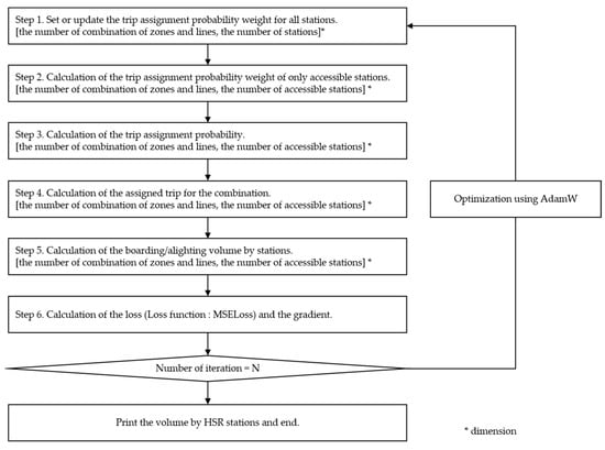
Figure 4.
The backpropagation-based optimization algorithm in this study.
The optimization calculation process is explained based on an example with a smaller dataset than the actual dataset used. The initial value of the trip assignment probability weight was constructed to be inversely proportional to the square of the Euclidean distance from zones to stations and proportional to the train frequency at the station, with reference to the gravity model [46]. The accessible stations were set to the three nearest stations.
First, to obtain the trip assignment probability weight tensor of only accessible stations, the probability weight tensor for all stations () with each combination of zones and lines is multiplied by the accessible station tensor (), where each entry has a value of 1 if the station is accessible; otherwise, it is 0 (a tensor refers to any data structure with a scalar, vector, matrix, or more dimensions). Accordingly, a trip assignment probability weight tensor () with only three accessible stations in its combinations remains, and the probability weights for all other stations become 0, as shown in Figure 5. This allows only three accessible stations for each combination to be included in the loss calculation and the probability weight updating process.

Figure 5.
Calculation of probability weight tensor ().
Since the probability weight tensor does not represent a probability, it must be converted into one using a normalization process, as shown in Figure 6. A row of the probability weight tensor () represents a combination of zones and lines, and a probability weight sum tensor () is created by extending a row-wise sum of the probability weight tensor. A probability tensor () is calculated by dividing the previous two tensors.

Figure 6.
Calculation converting the probability weight to the probability.
The following is the step used to assign the total trip from each combination of zones and lines to each station using the probability. The total trip tensor () is a tensor that contains the total trip information for each combination, and it is multiplied by the probability tensor () to obtain the assigned trip tensor () for the accessible stations. This is represented in Figure 7.

Figure 7.
Calculation used to assign the total trip values for each station using their respective probabilities.
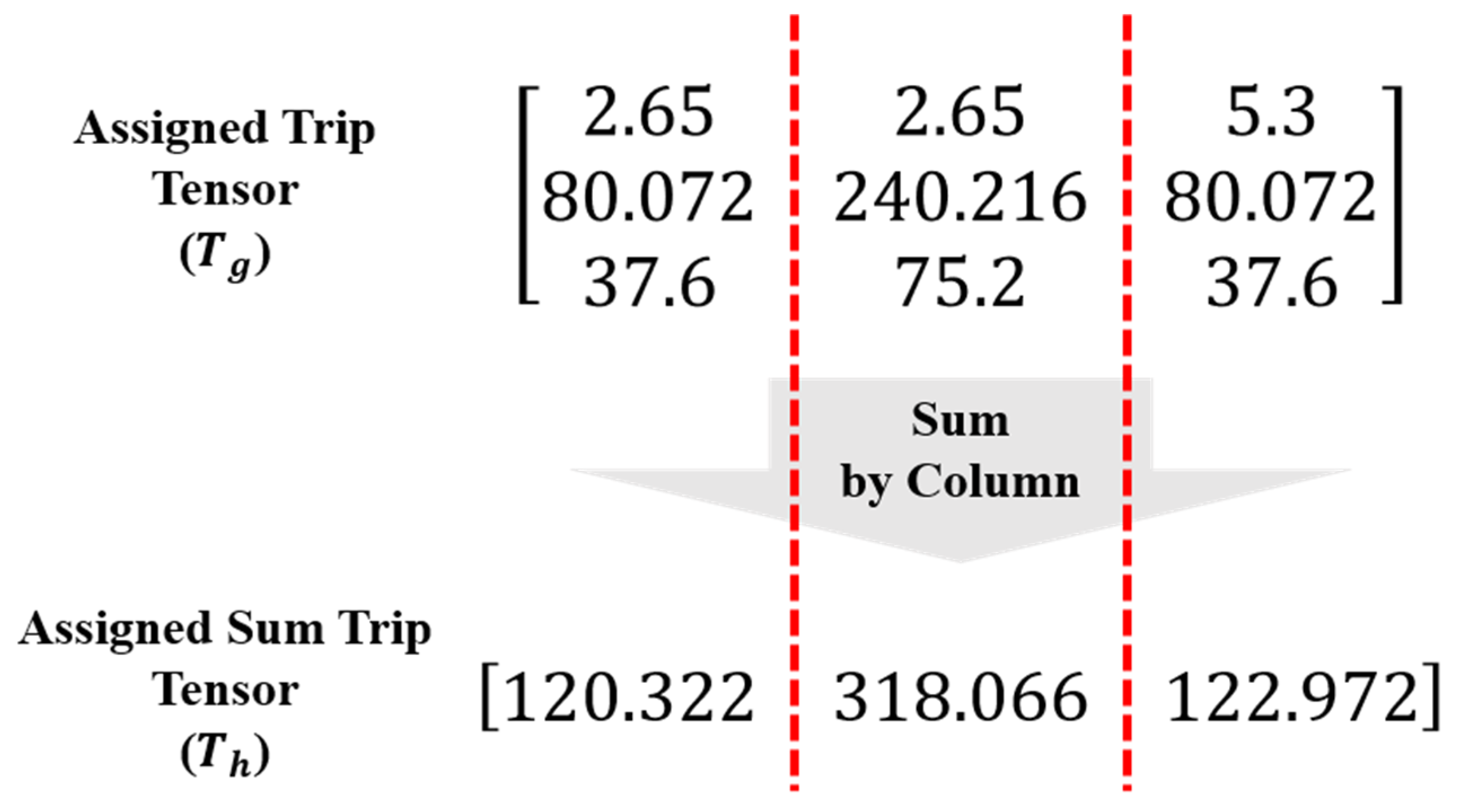
The boarding/alighting volume for each station must be estimated using the assigned trip tensor to calculate the loss compared with the observed volume. This is calculated by adding the entries in each column in the assigned trip tensor, as shown in Figure 8.
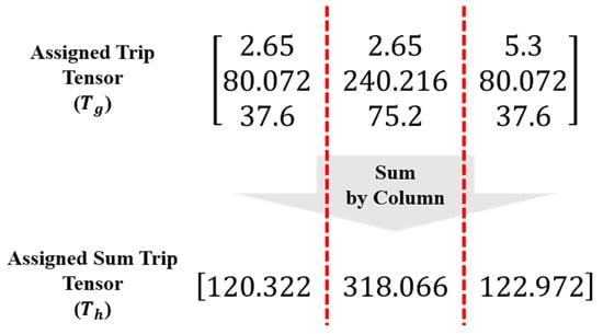
Figure 8.
Calculation of the boarding/alighting volume by stations.
The difference between the assigned sum trip tensor and the observed trip tensor is calculated with a predefined loss function. Finally, by calculating the gradient using backpropagation to reduce the loss, the probability weight tensor is updated until the end of the algorithm as shown in Figure A3. The optimization codes were implemented based on Python 3.8 and PyToch 1.11, and the PC specifications were CPU: Intel Core i5 11400 (2.60 GHz), memory: 32 GB, and GPU: NVIDIA GeForce RTX 2070 SUPER.
4. Case Study
4.1. Data Description
In Korea, the Korea Transport Institute (KOTI), a government-funded institute, periodically distributes KTDB data, including O/D trip and network data, to increase public confidence in long-term demand predictions. The KTDB data consist of 250 zones defined by local governments, and 247 zones were used in this study, as shown in Table 1; Jeju, Seogwipo, and Ulleung were excluded since they are islands that do not have HSR lines, and thus have zero trips.

Table 1.
Summary of zones in the KTDB data used in this study.
The O/D trip frequency in Korea’s HSR was 225,495 trips/day in 2018, and the number of inter-region (16 metropolitan local governments) O/D trips is shown in Table 2. There were no O/D trips between Gangwon and North/South Chungcheong, North/South Jeolla, and North/South Gyeongsang, as well as between North/South Jeolla and North/South Gyeongsang, in the KTDB. This is because travel between these regions is not directly connected by HSR, and thus travel time and distance between these regions is so long. Therefore, it was assumed that there was no transfer demand in the HSR network and only trips between stations connected by the same line.

Table 2.
Inter-region O/D trips in KTDB data.
The HSR network consists of railway stations and lines. There are 51 HSR stations and three major lines in Korea: Gyeongbu (Seoul–Busan), Honam (Seoul–Gwangju), and Gangneung (Seoul–Gangneung). Figure 9 shows HSR network data schematized using EMME, where the pink boxes represent the zones (centroids), and the blue lines represent the HSR lines.
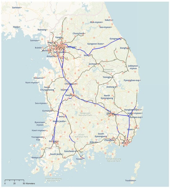
Figure 9.
HSR network data in the KTDB.
Two influential variables, namely the access distance from the zones to stations and the train frequency at the stations, were considered in this study. The access distance from zones to stations was calculated using the Euclidean distance from the centroid (a point representing each zone) to the station node. The KTDB network data used a local coordinate system (Bessel ellipsoid, Korean 1985 datum) to express the geographical location, and the coordinate system unit was in meters. Therefore, the Euclidean distance from zones to stations was calculated using Equation (2) [47]. The Euclidean distances were calculated by extracting only the information of the 51 HSR station nodes and 247 centroids in the KTDB network data.
Here,
- i: zone (i Z);
- s: HSR station (s S);
- : Euclidean distance from zone i to station s;
- x, y: x-coordinate and y-coordinate.
Sets
- Z: The set of zones;
- S: The set of HSR stations.
The train frequencies at the HSR stations were calculated by extracting the stop stations for each HSR train from the transit line data in the KTDB. Although both the skip and stop stations were presented in the transit line data, skip stations were excluded in the train frequency calculation, and the daily train frequency by line at the stations was calculated based on information for the line to which the train belonged.
4.2. Results
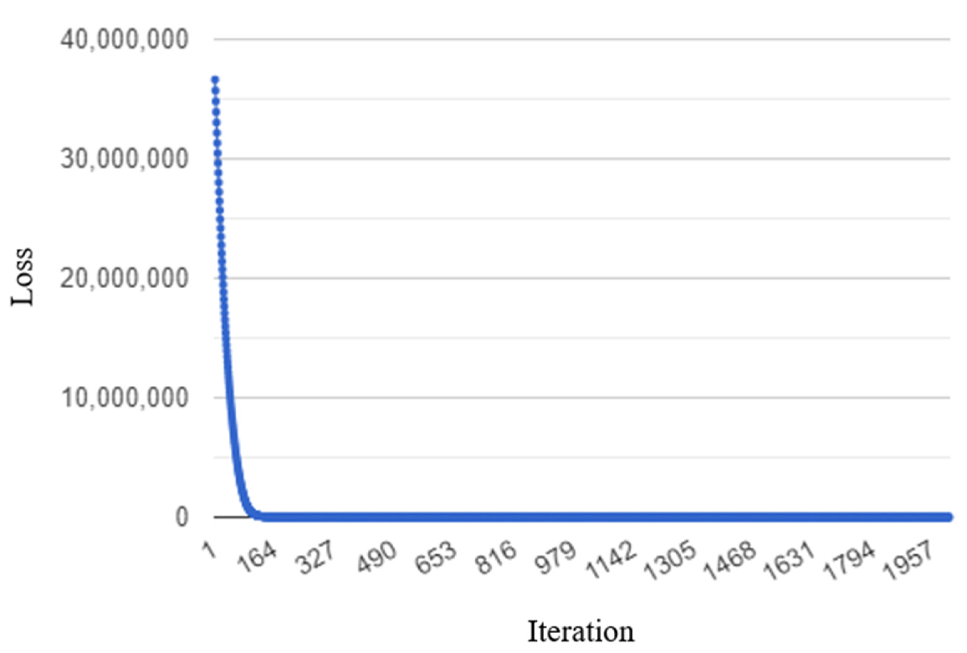
The trip assignment probability weight was updated 2000 times with a learning rate of 0.01 in the backpropagation-based algorithm. The loss had a downward trend with each update, and dropped sharply within about 200 iterations, as shown in Figure 10. Furthermore, it almost converged to the final value after about 200 iterations. When the probability weight was updated once, the loss was 36,624,504, and the final value decreased to 97,344 after 2000 iterations. This means that the difference between the estimated volume using the backpropagation-based algorithm and the observed volume significantly decreased.
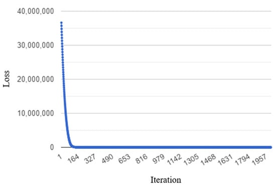
Figure 10.
The loss changes in the backpropagation-based algorithm by iteration.
The trip assignment results for each HSR station using the backpropagation-based algorithm are presented in Table 3. The results for major HSR stations with more than 1000 passengers are presented by dividing the regions into the Seoul metropolitan area, which had a relatively high concentration of HSR stations, and non-metropolitan areas, which did not. To verify the algorithm’s prediction performance, we compared the results found using the optimal strategy algorithm based on the volume at each HSR station. Moreover, the error rate presented in Equation (1) and the mean absolute error (MAE) and mean absolute percentage error (MAPE), expressed as Equation (3) [48], were chosen as the key performance indicators.

Table 3.
Trip assignment results for the major HSR stations.
Here,
- i: HSR station (i Z);
- n: the number of HSR stations;
- : the estimated number of passengers at each station using the trip assignment model;
- : the observed number of passengers at each station.
The trip assignment results from the backpropagation-based algorithm show that all stations had an error rate of less than 30%, the reference value stated by the guideline. However, the results from the optimal strategy algorithm show that many stations had an error rate exceeding 30%. The backpropagation-based algorithm results presented a very low error rate, less than 2% for the major stations with more than 10,000 passengers and less than 10% for the minor stations with less than 10,000 passengers. The high error rate at Gangneung Station could be attributed to the PyeongChang Olympic Winter Games. During the Winter Olympics, additional temporary trains that directly connected Incheon International Airport to Gangneung were operated. Accordingly, the observed volume at Gangneung Station was higher than usual; thus, the predicted demand was underestimated because it used the KTDB O/D trip data, estimated based on the average weekday trips.
The estimation accuracy using the backpropagation-based algorithm was relatively high compared with the estimation results from the optimal strategy algorithm for stations in both areas, i.e., the Seoul metropolitan area and the non-metropolitan area. However, the results for the Seoul metropolitan area show that the backpropagation-based algorithm’s accuracy was overwhelmingly higher than the optimal strategy algorithm’s accuracy. In the optimal strategy algorithm, the trip distribution among the adjacent stations was unbalanced, resulting in a large error rate. For example, in the Seoul metropolitan area, an error rate of more than 40% was found for Seoul, Cheongnyangni, and Haengsin Stations. Furthermore, in the non-metropolitan area, the demand that should have been assigned to Singyeongju Station was assigned to Ulsan Station, so the error rates were 19.2% and −42.2%, respectively, because the optimal strategy algorithm based on the all-or-nothing trip assignment was able to simulate the diverse access trip patterns of passengers in areas with multiple HSR stations, such as the Seoul metropolitan area. Therefore, after the initial assignment from the optimal strategy algorithm, it was necessary to reduce the error rate within the reference value using a parameter calibration process by adjusting the network parameters. The analyst’s arbitrary judgment was involved in this process, and much time and effort were required.
For stations in the Seoul metropolitan area, the MAE and MAPE indicators were 153 and 3.5%, respectively, when using the backpropagation-based algorithm, and those when using the optimal strategy algorithm were 3310 and 53.6%, respectively. Moreover, for the stations in the non-metropolitan area, the MAE and MAPE values were 123 and 1.8%, respectively, when using the backpropagation-based algorithm, and those when using the optimal strategy algorithm were 831 and 10.0%, respectively. Therefore, the estimation accuracy of the backpropagation-based algorithm developed in this study was superior to that of the optimal strategy algorithm.
5. Conclusions
We developed a backpropagation-based algorithm to optimize the trip assignment probability, and probability simulations of the access trip pattern from each zone to accessible HSR stations were undertaken. Backpropagation was used when training the artificial neural network; in this problem, the probability could be recognized as the weight optimized in the artificial neural network. Accordingly, the initial value in the backpropagation-based algorithm was a function of the access distance from zones to accessible HSR stations and the train frequency at HSR stations for each zone and line combination. The difference between the estimated volume from the probability and the observed volume was defined as the loss in the optimization process, and the weight was updated in the direction of minimizing this loss. To apply this backpropagation concept, we obtained the loss value using only differentiable calculations provided by PyTorch, a deep learning framework used for artificial neural network learning.
To verify the prediction performance of the backpropagation-based algorithm, its trip assignment results were compared with those of an optimal strategy algorithm using network and O/D trip data from the KTDB. A total of 225,495 trips/day generated from 247 zones were assigned to 51 stations on the three HSR lines. The results for 19 major HSR stations with more than 1000 passengers were presented by dividing the regions into the Seoul metropolitan area, which had a relatively high concentration of HSR stations, and a non-metropolitan area, which did not. The backpropagation-based algorithm results show that all stations had an error rate of less than 30%, the reference value stated in the guideline. Furthermore, the results present a very low error rate, less than 2% for major stations with more than 10,000 passengers and less than 10% for minor stations with less than 10,000 passengers. On the other hand, the optimal strategy algorithm results show that many stations had an error rate exceeding 30%. For the stations in the Seoul metropolitan area, the MAE and MAPE indicators found using the backpropagation-based algorithm were 153 and 3.5%, respectively, and those found using the optimal strategy algorithm were 3310 and 53.6%, respectively. This means that the backpropagation-based algorithm was especially superior when applied to an area with multiple HSR stations, simulating the passenger access trip pattern from each zone to multiple stations. Therefore, the backpropagation-based algorithm will improve the accuracy and time efficiency of long-term HSR demand forecasting.
A limitation of this study was that the access distance from each zone to the HSR stations was calculated using the Euclidean distance, which was used owing to data acquisition issues and the complexity problem of calculating using input data, such as applying the shortest path algorithm. If it were possible to obtain access distance or time data for each access mode to HSR stations, the algorithm’s accuracy would be improved by reflecting more realistic conditions. Lastly, it is necessary to examine the extendibility of the backpropagation-based algorithm by applying it to various HSR networks with different conditions from those in Korea.
Funding
This research received no external funding.
Institutional Review Board Statement
Not applicable.
Informed Consent Statement
Not applicable.
Data Availability Statement
The data are available upon request from the author.
Conflicts of Interest
The author declares no conflict of interest.
Appendix A
The main codes for optimizing the trip assignment probability weight are presented below. They consist of two steps: (1) variable initialization and (2) optimization.
- (1)
- Variable initialization
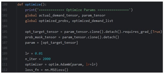
Figure A1.
The code for variable initialization.
Figure A1.
The code for variable initialization.
- (2)
- Optimization
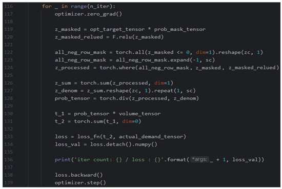
Figure A2.
The code for optimizing the trip assignment probability weight.
Figure A2.
The code for optimizing the trip assignment probability weight.
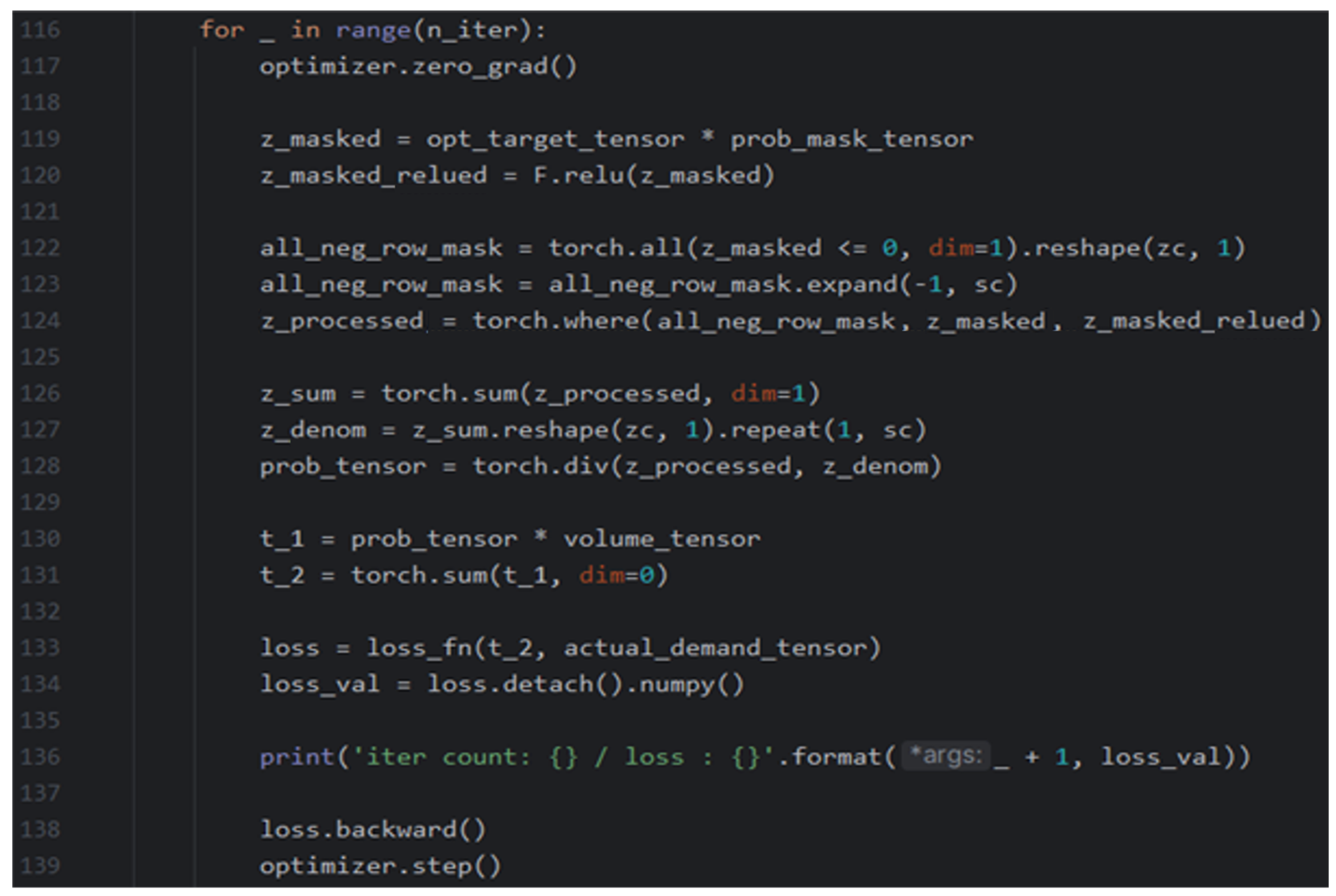

Figure A3.
The code for saving the optimized results after the last updating process.
Figure A3.
The code for saving the optimized results after the last updating process.

References
- International Union of Railways (UIC). High-Speed around the World; UIC Passenger Department: Paris, France, 2023; p. 6. ISBN 978-2-7461-3257-3. [Google Scholar]
- Kim, H.; Sultana, S. The impacts of high-speed rail extensions on accessibility and spatial equity changes in South Korea from 2004 to 2018. J. Transp. Geogr. 2015, 45, 48–61. [Google Scholar] [CrossRef]
- E-National Index Home Page. Available online: https://www.index.go.kr/unity/potal/main/EachDtlPageDetail.do?idx_cd=1252 (accessed on 1 August 2024).
- International Union of Railways (UIC). High Speed Rail: Fast Track to Sustainable Mobility; Passenger and High Speed Department: Paris, France, 2015; p. 3. ISBN 978-2-7461-1887-4. [Google Scholar]
- Korea Development Institute (KDI). The Guideline for Preliminary Feasibility Study in Road and Railway Sectors; KDI Public and Private Infrastructure Investment Management Center: Sejong, Republic of Korea, 2021. [Google Scholar]
- Dong, N.; Li, T.; Liu, T.; Tu, R.; Lin, F.; Liu, H.; Bo, Y. A method for short-term passenger flow prediction in urban rail transit based on deep learning. Multimed. Tools Appl. 2024, 83, 61621–61643. [Google Scholar] [CrossRef]
- Li, S.; Liang, X.; Zheng, M.; Chen, J.; Chen, T.; Guo, X. How spatial features affect urban rail transit prediction accuracy: A deep learning based passenger flow prediction method. J. Intell. Transp. Syst. 2023, 1–12. [Google Scholar] [CrossRef]
- He, Y.; Li, L.; Zhu, X.; Tsui, K.L. Multi-Graph Convolutional-Recurrent Neural Network (MGC-RNN) for Short-Term Forecasting of Transit Passenger Flow. IEEE Trans. Intell. Transp. Syst. 2022, 23, 18155–18174. [Google Scholar] [CrossRef]
- Zhang, J.; Chen, F.; Cui, Z.; Guo, Y.; Zhu, Y. Deep Learning Architecture for Short-Term Passenger Flow Forecasting in Urban Rail Transit. IEEE Trans. Intell. Transp. Syst. 2021, 22, 7004–7014. [Google Scholar] [CrossRef]
- Yang, X.; Xue, Q.; Ding, M.; Wu, J.; Gao, Z. Short-term prediction of passenger volume for urban rail systems: A deep learning approach based on smart-card data. Int. J. Prod. Econ. 2021, 231, 107920. [Google Scholar] [CrossRef]
- Zhang, H.; He, J.; Bao, J.; Hong, Q.; Shi, X. A Hybrid Spatiotemporal Deep Learning Model for Short-Term Metro Passenger Flow Prediction. J. Adv. Transp. 2020, 2020, 4656435. [Google Scholar] [CrossRef]
- Jia, H.; Luo, H.; Wang, H.; Zhao, F.; Ke, Q.; Wu, M.; Zhao, Y. ADST: Forecasting Metro Flow Using Attention-Based Deep Spatial-Temporal Networks with Multi-Task Learning. Sensors 2020, 20, 4574. [Google Scholar] [CrossRef]
- Zhang, J.; Chen, F.; Shen, Q. Cluster-Based LSTM Network for Short-Term Passenger Flow Forecasting in Urban Rail Transit. IEEE Access 2019, 7, 147653–147671. [Google Scholar] [CrossRef]
- Tang, Q.; Yang, M.; Yang, Y. ST-LSTM: A Deep Learning Approach Combined Spatio-Temporal Features for Short-Term Forecast in Rail Transit. J. Adv. Transp. 2019, 2019, 8392592. [Google Scholar] [CrossRef]
- Liu, Y.; Liu, Z.; Jia, R. DeepPF: A deep learning based architecture for metro passenger flow prediction. Transp. Res. Part C Emerg. Technol. 2019, 101, 18–34. [Google Scholar] [CrossRef]
- Ma, X.; Zhang, J.; Du, B.; Ding, C.; Sun, L. Parallel Architecture of Convolutional Bi-Directional LSTM Neural Networks for Network-Wide Metro Ridership Prediction. IEEE Trans. Intell. Transp. Syst. 2019, 20, 2278–2288. [Google Scholar] [CrossRef]
- Han, Y.; Wang, S.; Ren, Y.; Wang, C.; Gao, P.; Chen, G. Predicting Station-Level Short-Term Passenger Flow in a Citywide Metro Network Using Spatiotemporal Graph Convolution Neural Networks. ISPRS Int. J. Geo-Inf. 2019, 8, 243. [Google Scholar] [CrossRef]
- Hao, S.; Lee, D.-H.; Zhao, D. Sequence to sequence learning with attention mechanism for short-term passenger flow prediction in large-scale metro system. Transp. Res. Part C Emerg. Technol. 2019, 107, 287–300. [Google Scholar] [CrossRef]
- Wang, X.; Zhang, N.; Zhang, Y.; Shi, Z. Forecasting of Short-Term Metro Ridership with Support Vector Machine Online Model. J. Adv. Transp. 2018, 2018, 3189238. [Google Scholar] [CrossRef]
- Roos, J.; Gavin, G.; Bonnevay, S. A dynamic Bayesian network approach to forecast short-term urban rail passenger flows with incomplete data. Transp. Res. Procedia 2017, 26, 53–61. [Google Scholar] [CrossRef]
- Sun, Y.; Leng, B.; Guan, W. A novel wavelet-SVM short-time passenger flow prediction in Beijing subway system. Neurocomputing 2015, 166, 109–121. [Google Scholar] [CrossRef]
- Wei, Y.; Chen, M.-C. Forecasting the short-term metro passenger flow with empirical mode decomposition and neural networks. Transp. Res. Part C Emerg. Technol. 2012, 21, 148–162. [Google Scholar] [CrossRef]
- Liu, D.; Wu, Z.; Sun, S. Study on Subway passenger flow prediction based on deep recurrent neural network. Multimed. Tools Appl. 2022, 81, 18979–18992. [Google Scholar] [CrossRef]
- Guo, J.; Xie, Z.; Qin, Y.; Jia, L.; Wang, Y. Short-Term Abnormal Passenger Flow Prediction Based on the Fusion of SVR and LSTM. IEEE Access 2019, 7, 42946–42955. [Google Scholar] [CrossRef]
- Li, H.; Wang, Y.; Xu, X.; Qin, L.; Zhang, H. Short-term passenger flow prediction under passenger flow control using a dynamic radial basis function network. Appl. Soft Comput. 2019, 83, 105620. [Google Scholar] [CrossRef]
- Li, Y.; Wang, X.; Sun, S.; Ma, X.; Lu, G. Forecasting short-term subway passenger flow under special events scenarios using multiscale radial basis function networks. Transp. Res. Part C Emerg. Technol. 2017, 77, 306–328. [Google Scholar] [CrossRef]
- Zhao, S.; Mi, X. A Novel Hybrid Model for Short-Term High-Speed Railway Passenger Demand Forecasting. IEEE Access 2019, 7, 175681–175692. [Google Scholar] [CrossRef]
- Jiang, X.; Zhang, L.; Chen, X.M. Short-term forecasting of high-speed rail demand: A hybrid approach combining ensemble empirical mode decomposition and gray support vector machine with real-world applications in China. Transp. Res. Part C Emerg. Technol. 2014, 44, 110–127. [Google Scholar] [CrossRef]
- Du, Z.; Yang, W.; Yin, Y.; Ma, X.; Gong, J. Improved Long-Term Forecasting of Passenger Flow at Rail Transit Stations Based on an Artificial Neural Network. Appl. Sci. 2024, 14, 3100. [Google Scholar] [CrossRef]
- Lin, L.; Gao, Y.; Cao, B.; Wang, Z.; Jia, C. Passenger Flow Scale Prediction of Urban Rail Transit Stations Based on Multilayer Perceptron (MLP). Complexity 2023, 2023, 1430449. [Google Scholar] [CrossRef]
- Lin, C.; Wang, K.; Wu, D.; Gong, B. Passenger Flow Prediction Based on Land Use around Metro Stations: A Case Study. Sustainability 2020, 12, 6844. [Google Scholar] [CrossRef]
- Yu, H.-T.; Jiang, C.-J.; Xiao, R.-D.; Liu, H.-O.; Lv, W. Passenger Flow Prediction for New Line Using Region Dividing and Fuzzy Boundary Processing. IEEE Trans. Fuzzy Syst. 2019, 27, 994–1007. [Google Scholar] [CrossRef]
- He, Z.; Wang, B.; Huang, J.; Du, Y. Station passenger flow forecast for urban rail transit based on station attributes. In Proceedings of the IEEE 3rd International Conference on Cloud Computing and Intelligence Systems, Shenzhen, China, 27–29 November 2014; pp. 410–414. [Google Scholar] [CrossRef]
- Cao, W.; Sun, S.; Li, H. A new forecasting system for high-speed railway passenger demand based on residual component disposing. Measurement 2021, 183, 109762. [Google Scholar] [CrossRef]
- Börjesson, M. Forecasting demand for high speed rail. Transp. Res. Part A Policy Pract. 2014, 70, 81–92. [Google Scholar] [CrossRef]
- Tavassoli, A.; Mesbah, M.; Hickman, M. Calibrating a transit assignment model using smart card data in a large-scale multi-modal transit network. Transportation 2020, 47, 2133–2156. [Google Scholar] [CrossRef]
- Nassir, N.; Hickman, M.; Ma, Z. Statistical Inference of Transit Passenger Boarding Strategies from Farecard Data. Transp. Res. Rec. 2017, 2652, 8–18. [Google Scholar] [CrossRef]
- Spiess, H.; Florian, M. Optimal strategies: A new assignment model for transit networks. Transp. Res. Part B Methodol. 1989, 23, 83–102. [Google Scholar] [CrossRef]
- De Cea, J.; Fernandez, E. Transit Assignment for Congested Public Transport Systems: An Equilibrium Model. Transp. Sci. 1993, 37, 133–147. [Google Scholar] [CrossRef]
- Wu, J.H.; Florian, M.; Marcotte, P. Transit Equilibrium Assignment: A Model and Solution Algorithms. Transp. Sci. 1994, 28, 193–203. [Google Scholar] [CrossRef]
- Yao, E.; Morikawa, T. A study of on integrated intercity travel demand model. Transp. Res. Part A Policy Pract. 2005, 39, 367–381. [Google Scholar] [CrossRef]
- Choi, J.; Lee, Y.J.; Kim, T.; Sohn, K. An analysis of Metro ridership at the station-to-station level in Seoul. Transportation 2012, 39, 705–722. [Google Scholar] [CrossRef]
- Schmidhuber, J. Deep learning in neural networks: An overview. Neural Netw. 2015, 61, 85–117. [Google Scholar] [CrossRef]
- Paszke, A.; Gross, S.; Chintala, S.; Chanan, G.; Yang, E.; DeVito, Z.; Lin, Z.; Desmaison, A.; Antiga, L.; Lerer, A. Automatic differentiation in PyTorch. In Proceedings of the 31st Conference on Neural Information Processing Systems (NIPS 2017), Long Beach, CA, USA, 4–9 December 2017. [Google Scholar]
- Loshchilov, I.; Hutter, F. Decoupled Weight Decay Regularization. arXiv 2017, arXiv:1711.05101. [Google Scholar]
- Wilson, A.G. A statistical theory of spatial distribution models. Transp. Res. 1967, 1, 253–269. [Google Scholar] [CrossRef]
- Cohen, D. Precalculus: A Problems-Oriented Approach, 6th ed.; Cengage Learning: Belmont, CA, USA, 2004; p. 698. ISBN 978-0-534-40212-9. [Google Scholar]
- Ma, Z.; Xing, J.; Mesbah, M.; Ferreira, L. Predicting short-term bus passenger demand using a pattern hybrid approach. Transp. Res. Part C Emerg. Technol. 2014, 39, 148–163. [Google Scholar] [CrossRef]
Disclaimer/Publisher’s Note: The statements, opinions and data contained in all publications are solely those of the individual author(s) and contributor(s) and not of MDPI and/or the editor(s). MDPI and/or the editor(s) disclaim responsibility for any injury to people or property resulting from any ideas, methods, instructions or products referred to in the content. |
© 2024 by the author. Licensee MDPI, Basel, Switzerland. This article is an open access article distributed under the terms and conditions of the Creative Commons Attribution (CC BY) license (https://creativecommons.org/licenses/by/4.0/).

