
A Backpropagation-Based Algorithm to Optimize Trip Assignment Probability for Long-Term High-Speed Railway Demand Forecasting in Korea
Abstract
:Featured Application
Abstract
1. Introduction
- Define a departure node (station or stop);
- Move to and board the vehicle that arrives first at the departure node among the competing routes;
- Get off at the intermediate node (station or stop) that was determined according to the optimal strategy;
- End if the passenger arrives at their destination; otherwise, define the alighting node as the departure node and repeat from step 1.
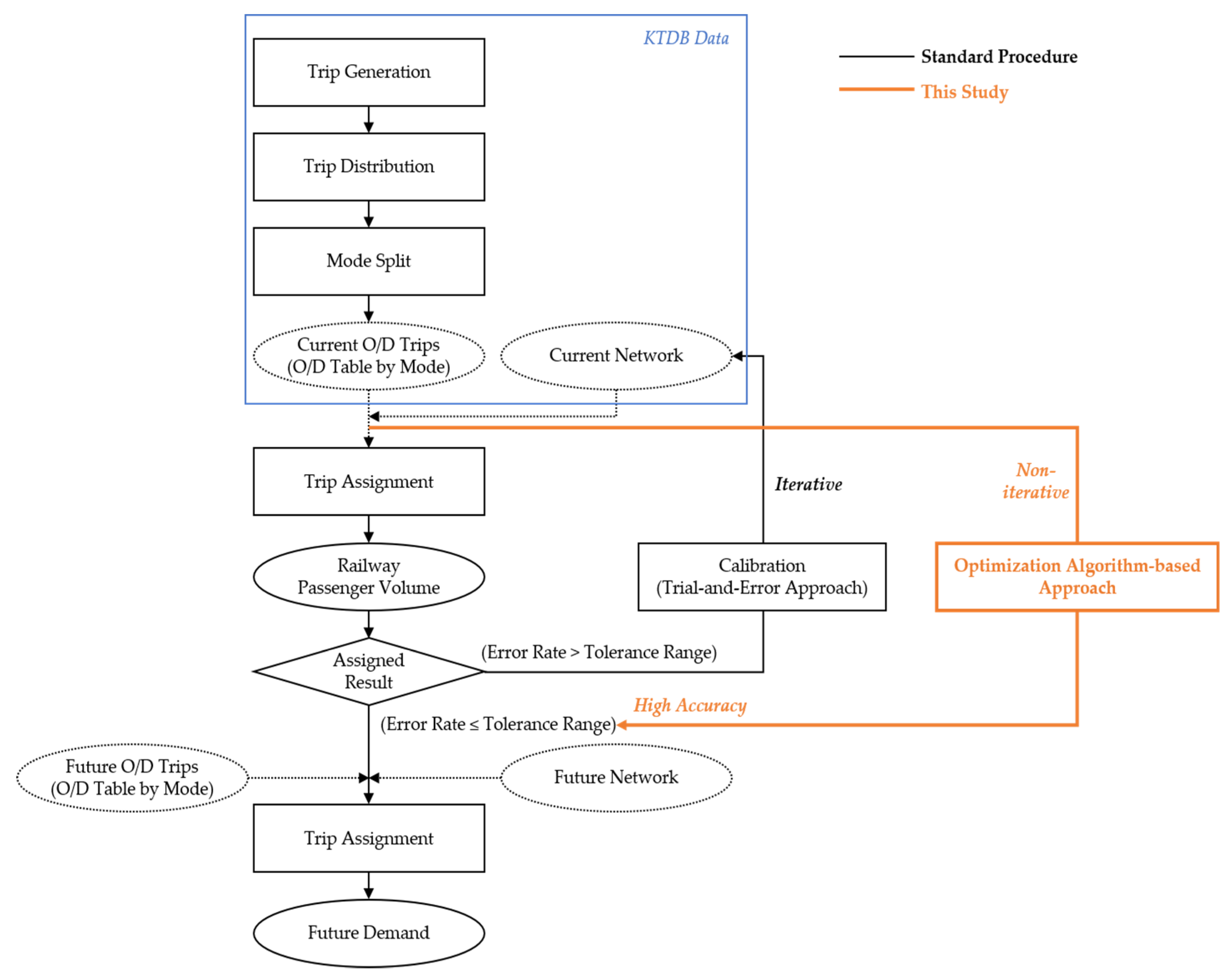
2. Standard Long-Term HSR Demand-Forecasting Methodology in Korea
3. Methods
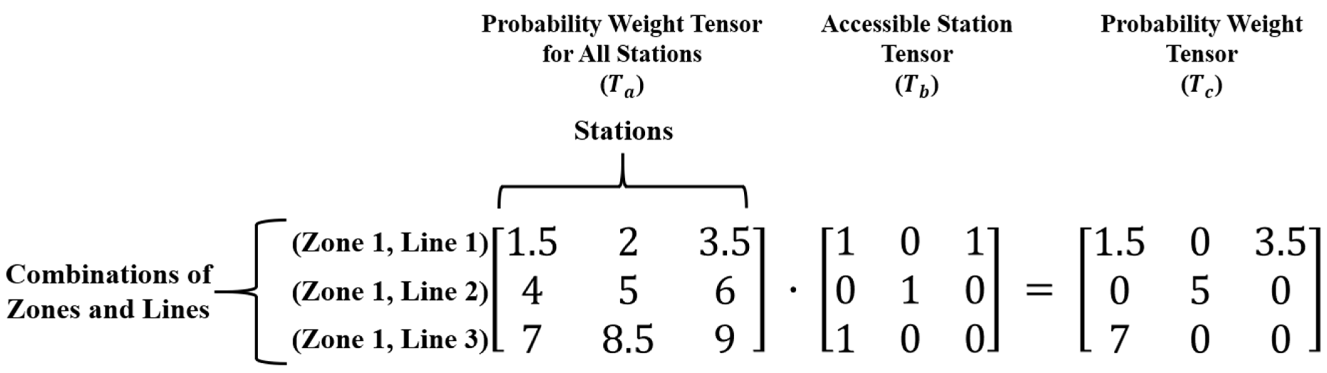
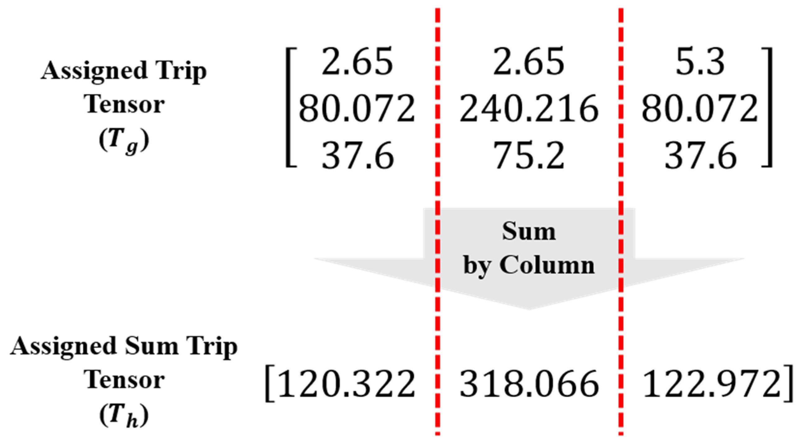
3.1. Trip Assignment Probability
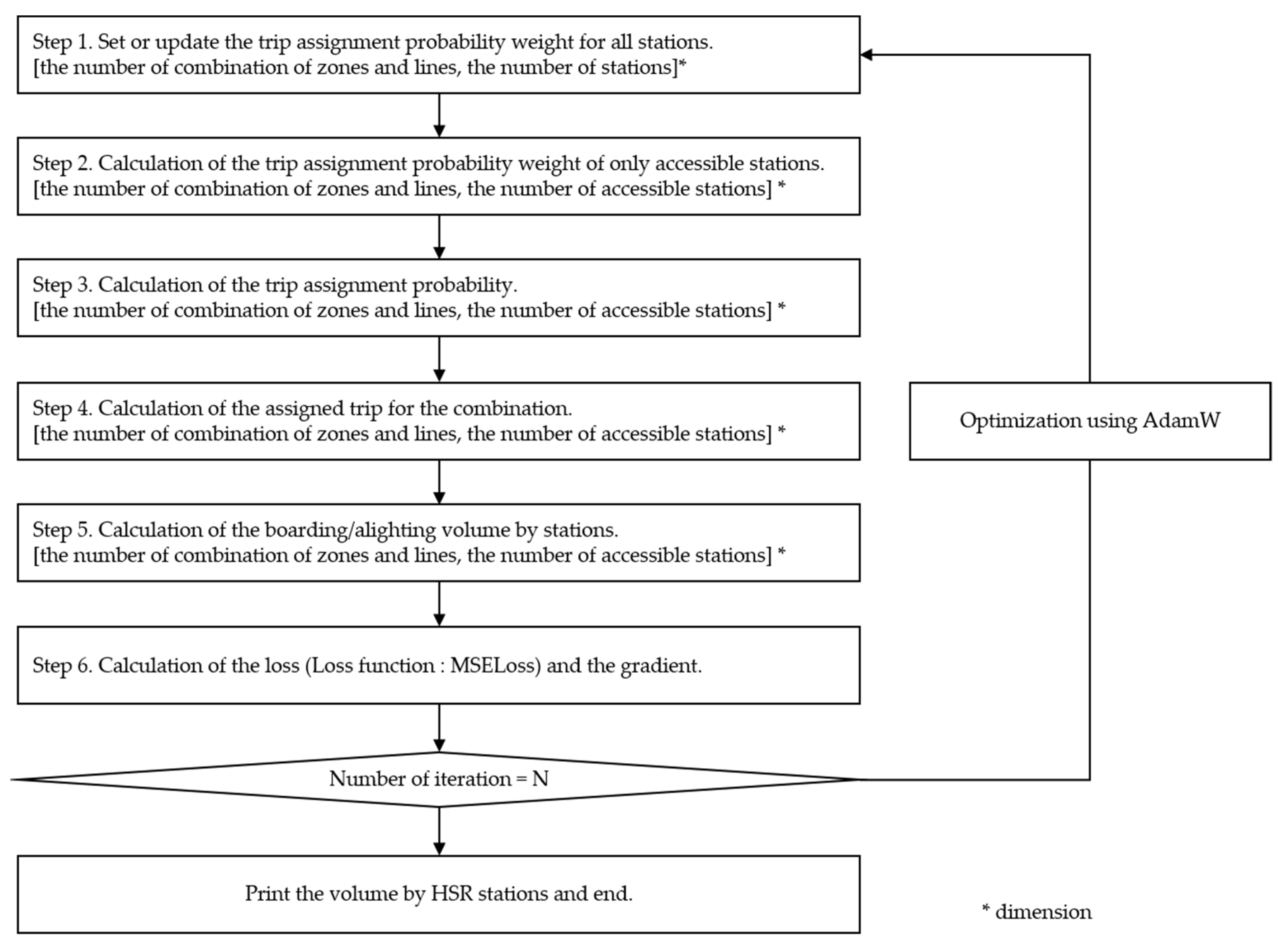
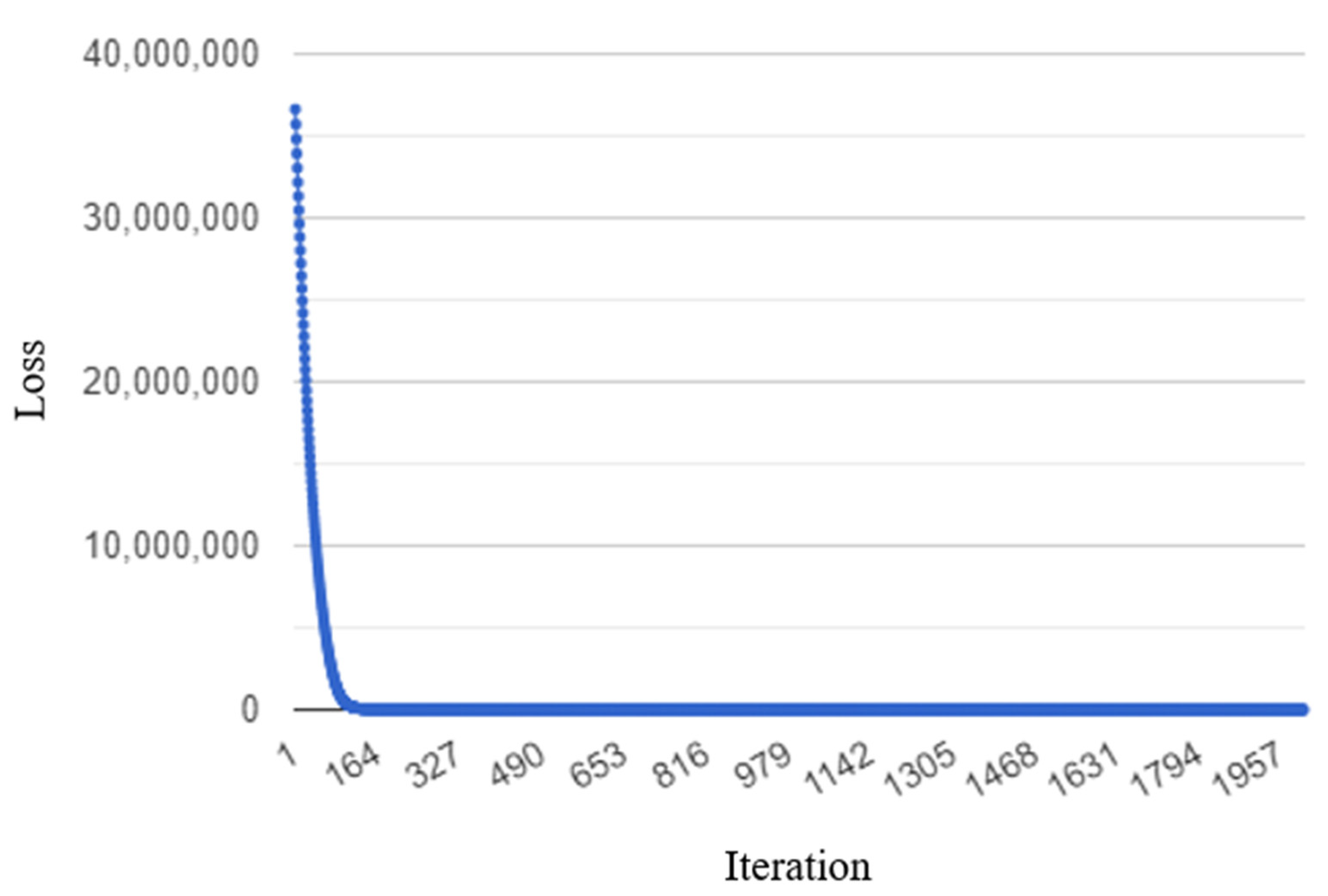
3.2. Optimization Algorithm
4. Case Study
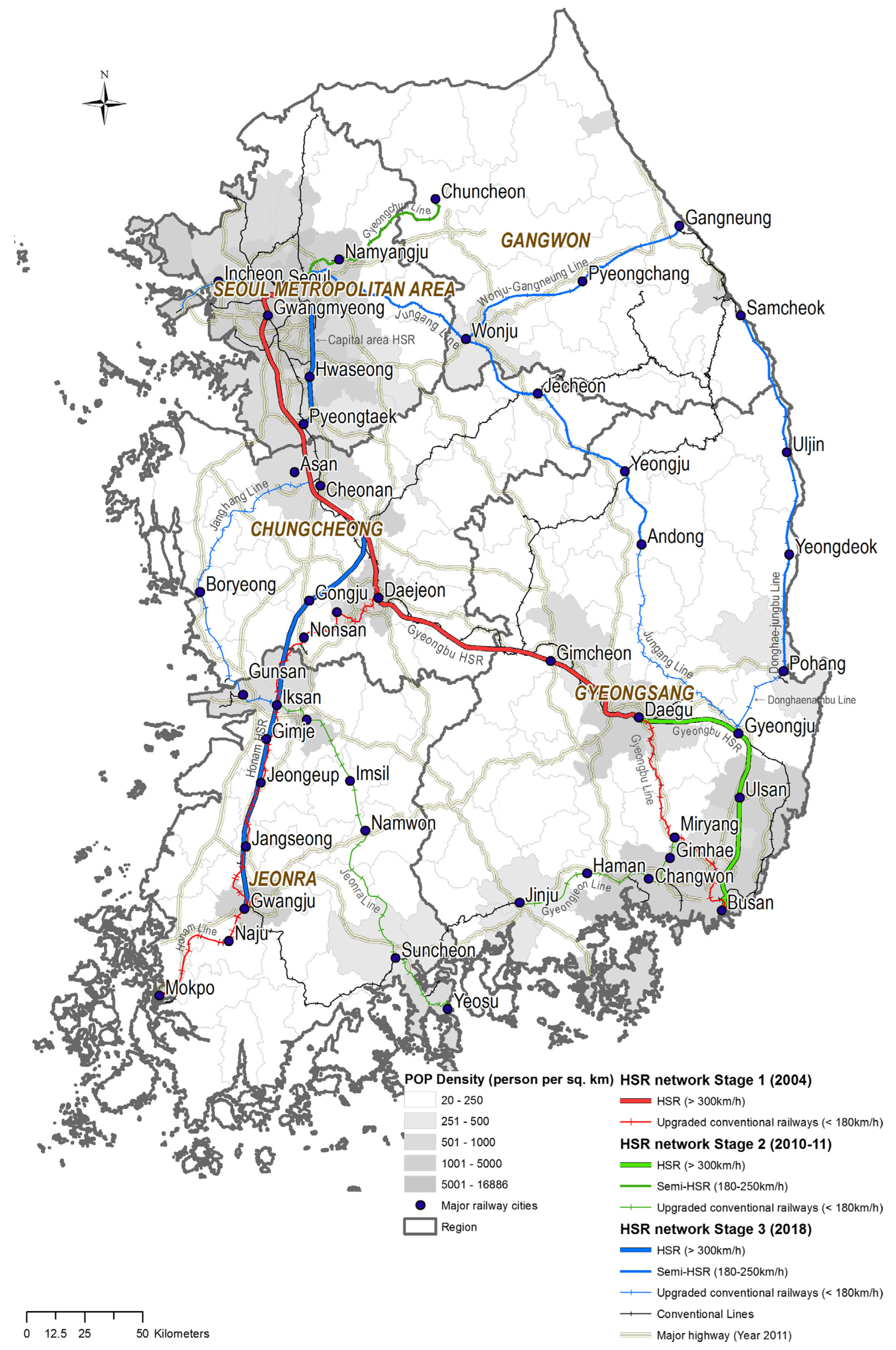
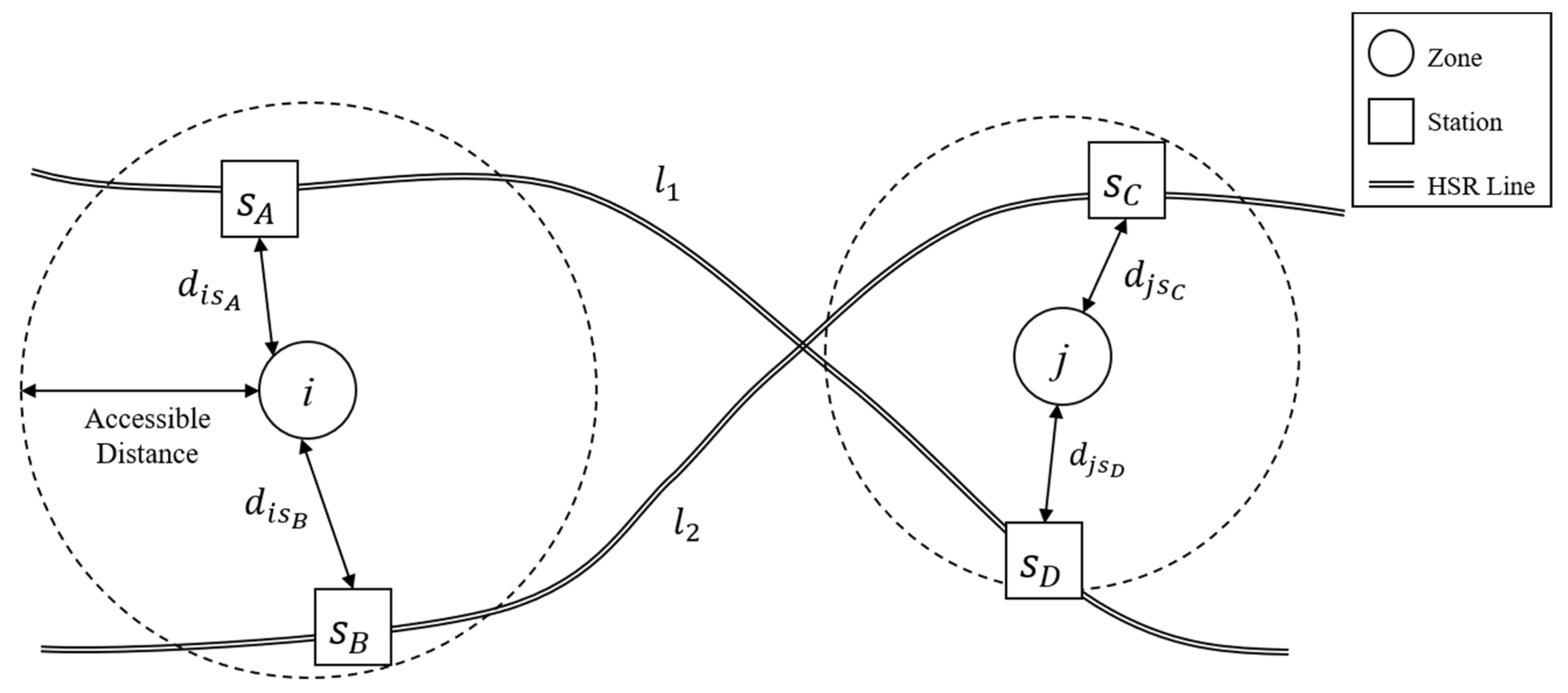
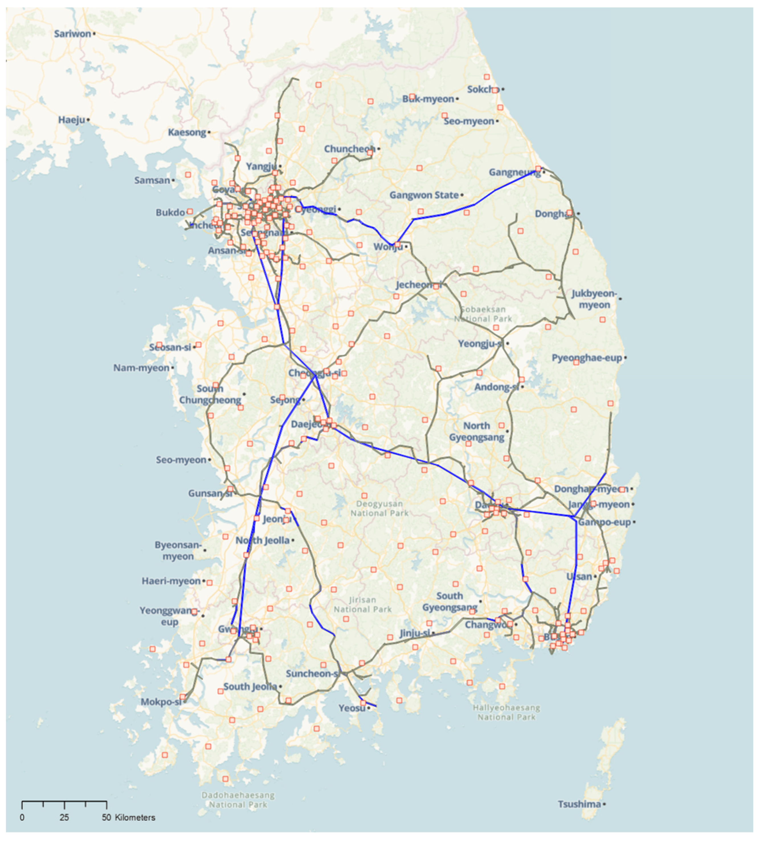
4.1. Data Description
- i: zone (i Z);
- s: HSR station (s S);
- : Euclidean distance from zone i to station s;
- x, y: x-coordinate and y-coordinate.
- Z: The set of zones;
- S: The set of HSR stations.
4.2. Results
- i: HSR station (i Z);
- n: the number of HSR stations;
- : the estimated number of passengers at each station using the trip assignment model;
- : the observed number of passengers at each station.
5. Conclusions
Funding
Institutional Review Board Statement
Informed Consent Statement
Data Availability Statement
Conflicts of Interest
Appendix A
- (1)
- Variable initialization
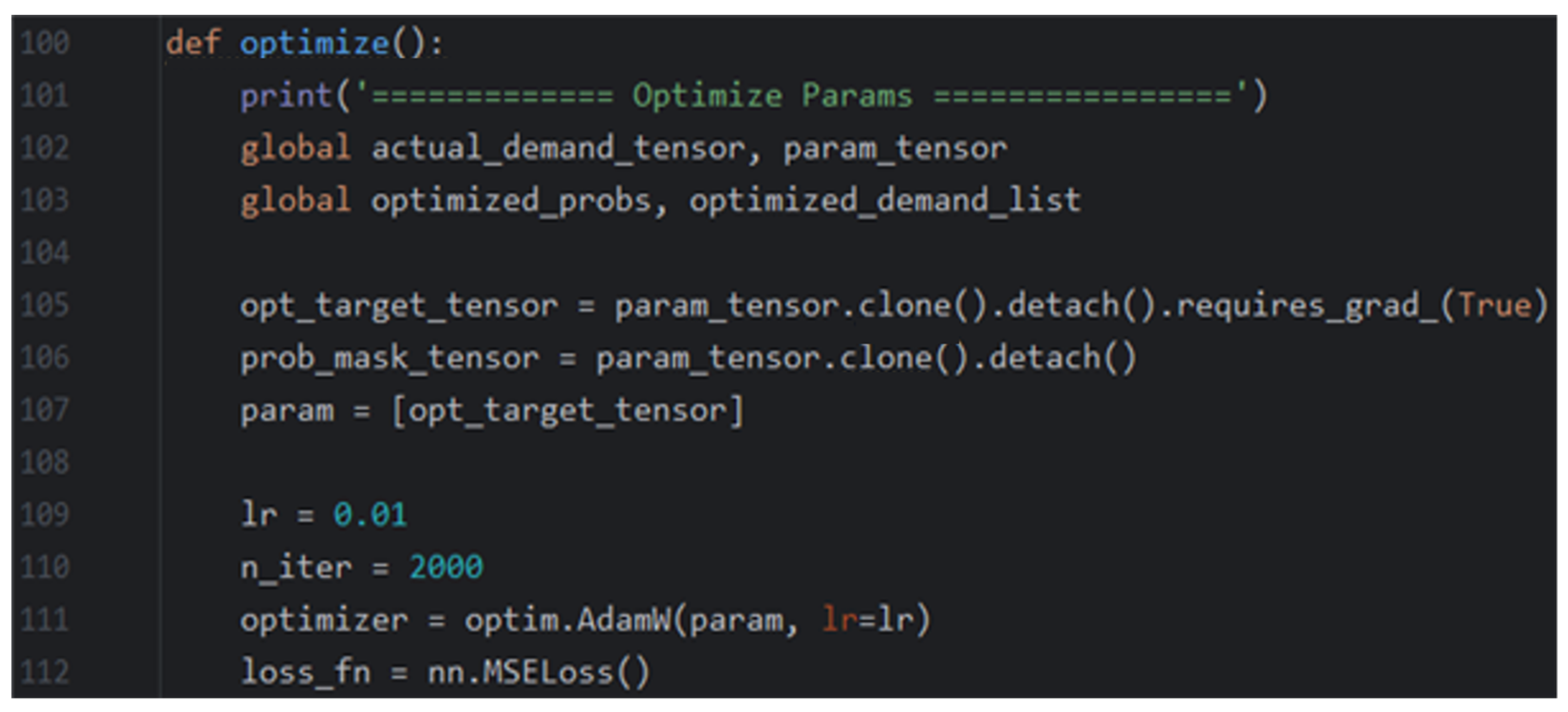
- (2)
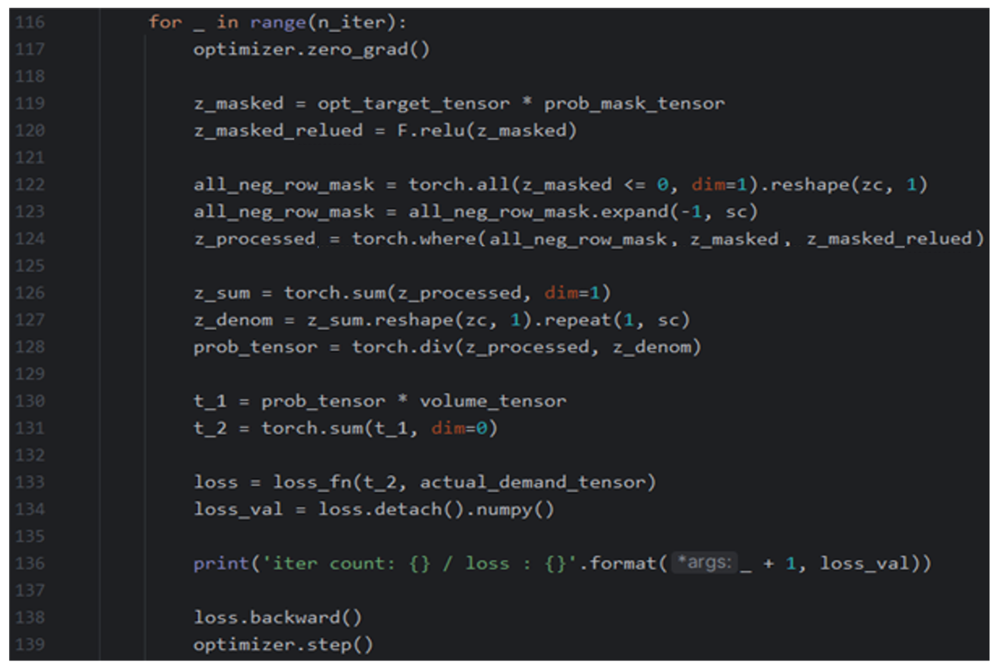
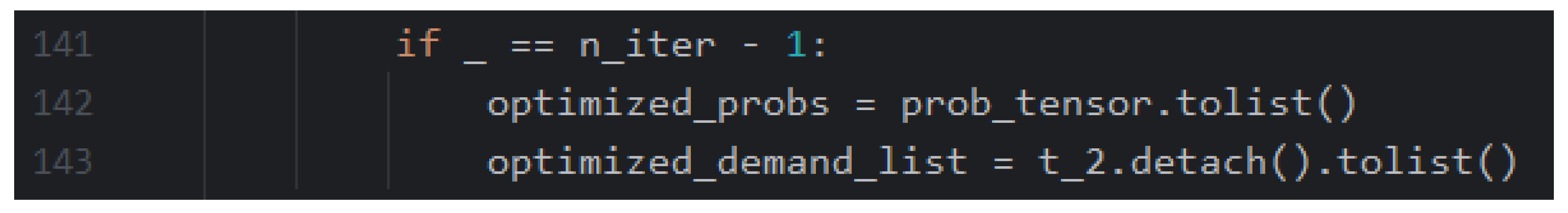
- Optimization
References
- International Union of Railways (UIC). High-Speed around the World; UIC Passenger Department: Paris, France, 2023; p. 6. ISBN 978-2-7461-3257-3. [Google Scholar]
- Kim, H.; Sultana, S. The impacts of high-speed rail extensions on accessibility and spatial equity changes in South Korea from 2004 to 2018. J. Transp. Geogr. 2015, 45, 48–61. [Google Scholar] [CrossRef]
- E-National Index Home Page. Available online: https://www.index.go.kr/unity/potal/main/EachDtlPageDetail.do?idx_cd=1252 (accessed on 1 August 2024).
- International Union of Railways (UIC). High Speed Rail: Fast Track to Sustainable Mobility; Passenger and High Speed Department: Paris, France, 2015; p. 3. ISBN 978-2-7461-1887-4. [Google Scholar]
- Korea Development Institute (KDI). The Guideline for Preliminary Feasibility Study in Road and Railway Sectors; KDI Public and Private Infrastructure Investment Management Center: Sejong, Republic of Korea, 2021. [Google Scholar]
- Dong, N.; Li, T.; Liu, T.; Tu, R.; Lin, F.; Liu, H.; Bo, Y. A method for short-term passenger flow prediction in urban rail transit based on deep learning. Multimed. Tools Appl. 2024, 83, 61621–61643. [Google Scholar] [CrossRef]
- Li, S.; Liang, X.; Zheng, M.; Chen, J.; Chen, T.; Guo, X. How spatial features affect urban rail transit prediction accuracy: A deep learning based passenger flow prediction method. J. Intell. Transp. Syst. 2023, 1–12. [Google Scholar] [CrossRef]
- He, Y.; Li, L.; Zhu, X.; Tsui, K.L. Multi-Graph Convolutional-Recurrent Neural Network (MGC-RNN) for Short-Term Forecasting of Transit Passenger Flow. IEEE Trans. Intell. Transp. Syst. 2022, 23, 18155–18174. [Google Scholar] [CrossRef]
- Zhang, J.; Chen, F.; Cui, Z.; Guo, Y.; Zhu, Y. Deep Learning Architecture for Short-Term Passenger Flow Forecasting in Urban Rail Transit. IEEE Trans. Intell. Transp. Syst. 2021, 22, 7004–7014. [Google Scholar] [CrossRef]
- Yang, X.; Xue, Q.; Ding, M.; Wu, J.; Gao, Z. Short-term prediction of passenger volume for urban rail systems: A deep learning approach based on smart-card data. Int. J. Prod. Econ. 2021, 231, 107920. [Google Scholar] [CrossRef]
- Zhang, H.; He, J.; Bao, J.; Hong, Q.; Shi, X. A Hybrid Spatiotemporal Deep Learning Model for Short-Term Metro Passenger Flow Prediction. J. Adv. Transp. 2020, 2020, 4656435. [Google Scholar] [CrossRef]
- Jia, H.; Luo, H.; Wang, H.; Zhao, F.; Ke, Q.; Wu, M.; Zhao, Y. ADST: Forecasting Metro Flow Using Attention-Based Deep Spatial-Temporal Networks with Multi-Task Learning. Sensors 2020, 20, 4574. [Google Scholar] [CrossRef]
- Zhang, J.; Chen, F.; Shen, Q. Cluster-Based LSTM Network for Short-Term Passenger Flow Forecasting in Urban Rail Transit. IEEE Access 2019, 7, 147653–147671. [Google Scholar] [CrossRef]
- Tang, Q.; Yang, M.; Yang, Y. ST-LSTM: A Deep Learning Approach Combined Spatio-Temporal Features for Short-Term Forecast in Rail Transit. J. Adv. Transp. 2019, 2019, 8392592. [Google Scholar] [CrossRef]
- Liu, Y.; Liu, Z.; Jia, R. DeepPF: A deep learning based architecture for metro passenger flow prediction. Transp. Res. Part C Emerg. Technol. 2019, 101, 18–34. [Google Scholar] [CrossRef]
- Ma, X.; Zhang, J.; Du, B.; Ding, C.; Sun, L. Parallel Architecture of Convolutional Bi-Directional LSTM Neural Networks for Network-Wide Metro Ridership Prediction. IEEE Trans. Intell. Transp. Syst. 2019, 20, 2278–2288. [Google Scholar] [CrossRef]
- Han, Y.; Wang, S.; Ren, Y.; Wang, C.; Gao, P.; Chen, G. Predicting Station-Level Short-Term Passenger Flow in a Citywide Metro Network Using Spatiotemporal Graph Convolution Neural Networks. ISPRS Int. J. Geo-Inf. 2019, 8, 243. [Google Scholar] [CrossRef]
- Hao, S.; Lee, D.-H.; Zhao, D. Sequence to sequence learning with attention mechanism for short-term passenger flow prediction in large-scale metro system. Transp. Res. Part C Emerg. Technol. 2019, 107, 287–300. [Google Scholar] [CrossRef]
- Wang, X.; Zhang, N.; Zhang, Y.; Shi, Z. Forecasting of Short-Term Metro Ridership with Support Vector Machine Online Model. J. Adv. Transp. 2018, 2018, 3189238. [Google Scholar] [CrossRef]
- Roos, J.; Gavin, G.; Bonnevay, S. A dynamic Bayesian network approach to forecast short-term urban rail passenger flows with incomplete data. Transp. Res. Procedia 2017, 26, 53–61. [Google Scholar] [CrossRef]
- Sun, Y.; Leng, B.; Guan, W. A novel wavelet-SVM short-time passenger flow prediction in Beijing subway system. Neurocomputing 2015, 166, 109–121. [Google Scholar] [CrossRef]
- Wei, Y.; Chen, M.-C. Forecasting the short-term metro passenger flow with empirical mode decomposition and neural networks. Transp. Res. Part C Emerg. Technol. 2012, 21, 148–162. [Google Scholar] [CrossRef]
- Liu, D.; Wu, Z.; Sun, S. Study on Subway passenger flow prediction based on deep recurrent neural network. Multimed. Tools Appl. 2022, 81, 18979–18992. [Google Scholar] [CrossRef]
- Guo, J.; Xie, Z.; Qin, Y.; Jia, L.; Wang, Y. Short-Term Abnormal Passenger Flow Prediction Based on the Fusion of SVR and LSTM. IEEE Access 2019, 7, 42946–42955. [Google Scholar] [CrossRef]
- Li, H.; Wang, Y.; Xu, X.; Qin, L.; Zhang, H. Short-term passenger flow prediction under passenger flow control using a dynamic radial basis function network. Appl. Soft Comput. 2019, 83, 105620. [Google Scholar] [CrossRef]
- Li, Y.; Wang, X.; Sun, S.; Ma, X.; Lu, G. Forecasting short-term subway passenger flow under special events scenarios using multiscale radial basis function networks. Transp. Res. Part C Emerg. Technol. 2017, 77, 306–328. [Google Scholar] [CrossRef]
- Zhao, S.; Mi, X. A Novel Hybrid Model for Short-Term High-Speed Railway Passenger Demand Forecasting. IEEE Access 2019, 7, 175681–175692. [Google Scholar] [CrossRef]
- Jiang, X.; Zhang, L.; Chen, X.M. Short-term forecasting of high-speed rail demand: A hybrid approach combining ensemble empirical mode decomposition and gray support vector machine with real-world applications in China. Transp. Res. Part C Emerg. Technol. 2014, 44, 110–127. [Google Scholar] [CrossRef]
- Du, Z.; Yang, W.; Yin, Y.; Ma, X.; Gong, J. Improved Long-Term Forecasting of Passenger Flow at Rail Transit Stations Based on an Artificial Neural Network. Appl. Sci. 2024, 14, 3100. [Google Scholar] [CrossRef]
- Lin, L.; Gao, Y.; Cao, B.; Wang, Z.; Jia, C. Passenger Flow Scale Prediction of Urban Rail Transit Stations Based on Multilayer Perceptron (MLP). Complexity 2023, 2023, 1430449. [Google Scholar] [CrossRef]
- Lin, C.; Wang, K.; Wu, D.; Gong, B. Passenger Flow Prediction Based on Land Use around Metro Stations: A Case Study. Sustainability 2020, 12, 6844. [Google Scholar] [CrossRef]
- Yu, H.-T.; Jiang, C.-J.; Xiao, R.-D.; Liu, H.-O.; Lv, W. Passenger Flow Prediction for New Line Using Region Dividing and Fuzzy Boundary Processing. IEEE Trans. Fuzzy Syst. 2019, 27, 994–1007. [Google Scholar] [CrossRef]
- He, Z.; Wang, B.; Huang, J.; Du, Y. Station passenger flow forecast for urban rail transit based on station attributes. In Proceedings of the IEEE 3rd International Conference on Cloud Computing and Intelligence Systems, Shenzhen, China, 27–29 November 2014; pp. 410–414. [Google Scholar] [CrossRef]
- Cao, W.; Sun, S.; Li, H. A new forecasting system for high-speed railway passenger demand based on residual component disposing. Measurement 2021, 183, 109762. [Google Scholar] [CrossRef]
- Börjesson, M. Forecasting demand for high speed rail. Transp. Res. Part A Policy Pract. 2014, 70, 81–92. [Google Scholar] [CrossRef]
- Tavassoli, A.; Mesbah, M.; Hickman, M. Calibrating a transit assignment model using smart card data in a large-scale multi-modal transit network. Transportation 2020, 47, 2133–2156. [Google Scholar] [CrossRef]
- Nassir, N.; Hickman, M.; Ma, Z. Statistical Inference of Transit Passenger Boarding Strategies from Farecard Data. Transp. Res. Rec. 2017, 2652, 8–18. [Google Scholar] [CrossRef]
- Spiess, H.; Florian, M. Optimal strategies: A new assignment model for transit networks. Transp. Res. Part B Methodol. 1989, 23, 83–102. [Google Scholar] [CrossRef]
- De Cea, J.; Fernandez, E. Transit Assignment for Congested Public Transport Systems: An Equilibrium Model. Transp. Sci. 1993, 37, 133–147. [Google Scholar] [CrossRef]
- Wu, J.H.; Florian, M.; Marcotte, P. Transit Equilibrium Assignment: A Model and Solution Algorithms. Transp. Sci. 1994, 28, 193–203. [Google Scholar] [CrossRef]
- Yao, E.; Morikawa, T. A study of on integrated intercity travel demand model. Transp. Res. Part A Policy Pract. 2005, 39, 367–381. [Google Scholar] [CrossRef]
- Choi, J.; Lee, Y.J.; Kim, T.; Sohn, K. An analysis of Metro ridership at the station-to-station level in Seoul. Transportation 2012, 39, 705–722. [Google Scholar] [CrossRef]
- Schmidhuber, J. Deep learning in neural networks: An overview. Neural Netw. 2015, 61, 85–117. [Google Scholar] [CrossRef]
- Paszke, A.; Gross, S.; Chintala, S.; Chanan, G.; Yang, E.; DeVito, Z.; Lin, Z.; Desmaison, A.; Antiga, L.; Lerer, A. Automatic differentiation in PyTorch. In Proceedings of the 31st Conference on Neural Information Processing Systems (NIPS 2017), Long Beach, CA, USA, 4–9 December 2017. [Google Scholar]
- Loshchilov, I.; Hutter, F. Decoupled Weight Decay Regularization. arXiv 2017, arXiv:1711.05101. [Google Scholar]
- Wilson, A.G. A statistical theory of spatial distribution models. Transp. Res. 1967, 1, 253–269. [Google Scholar] [CrossRef]
- Cohen, D. Precalculus: A Problems-Oriented Approach, 6th ed.; Cengage Learning: Belmont, CA, USA, 2004; p. 698. ISBN 978-0-534-40212-9. [Google Scholar]
- Ma, Z.; Xing, J.; Mesbah, M.; Ferreira, L. Predicting short-term bus passenger demand using a pattern hybrid approach. Transp. Res. Part C Emerg. Technol. 2014, 39, 148–163. [Google Scholar] [CrossRef]


| Region | No. of Zones | Region | No. of Zones | Region | No. of Zones | Region | No. of Zones |
|---|---|---|---|---|---|---|---|
| Seoul | 25 | Gwangju | 5 | Gangwon | 18 | Jeonnam | 22 |
| Busan | 16 | Daejeon | 5 | Chungbuk | 14 | Gyeongbuk | 24 |
| Daegu | 7 | Ulsan | 5 | Chungnam | 16 | Gyeongnam | 22 |
| Incheon | 10 | Gyeonggi | 42 | Jeonbuk | 15 | Sejong | 1 |
| O/D | Seoul | Busan | Daegu | Incheon | Gwangju | Daejeon | Ulsan | Gyeonggi |
| Seoul | 16 | 10,480 | 7938 | 237 | 4493 | 7529 | 2865 | 1418 |
| Busan | 10,030 | 15 | 1849 | 712 | 0 | 1724 | 656 | 4220 |
| Daegu | 7953 | 2021 | 0 | 593 | 0 | 1461 | 956 | 3311 |
| Incheon | 729 | 737 | 585 | 0 | 295 | 570 | 243 | 2 |
| Gwangju | 4511 | 0 | 0 | 295 | 0 | 30 | 0 | 1761 |
| Daejeon | 7597 | 1925 | 1527 | 577 | 38 | 0 | 681 | 2527 |
| Ulsan | 2939 | 741 | 844 | 251 | 0 | 678 | 55 | 1329 |
| Gyeonggi | 1324 | 4468 | 3404 | 3 | 1763 | 2619 | 1292 | 304 |
| Gangwon | 3406 | 0 | 0 | 128 | 0 | 0 | 0 | 573 |
| North Chungcheong | 2467 | 339 | 250 | 185 | 179 | 220 | 113 | 754 |
| South Chungcheong | 4766 | 905 | 742 | 364 | 329 | 1241 | 423 | 1538 |
| North Jeolla | 3882 | 0 | 0 | 286 | 500 | 94 | 0 | 1393 |
| South Jeolla | 3886 | 0 | 0 | 328 | 324 | 66 | 0 | 1386 |
| North Gyeongsang | 3914 | 547 | 1244 | 340 | 0 | 992 | 119 | 1437 |
| South Gyeongsang | 2482 | 55 | 817 | 261 | 0 | 593 | 0 | 868 |
| Sejong | 2642 | 363 | 268 | 198 | 191 | 40 | 121 | 808 |
| O/D | Gangwon | North Chungcheong | South Chungcheong | North Jeolla | South Jeolla | North Gyeongsang | South Gyeongsang | Sejong |
| Seoul | 3435 | 2385 | 5141 | 3811 | 3847 | 3876 | 2419 | 2554 |
| Busan | 0 | 320 | 801 | 0 | 0 | 517 | 47 | 343 |
| Daegu | 0 | 244 | 679 | 0 | 0 | 1318 | 781 | 262 |
| Incheon | 118 | 187 | 411 | 287 | 333 | 338 | 256 | 200 |
| Gwangju | 0 | 169 | 299 | 509 | 438 | 0 | 0 | 181 |
| Daejeon | 0 | 10 | 1231 | 128 | 93 | 1049 | 559 | 275 |
| Ulsan | 0 | 114 | 403 | 0 | 0 | 117 | 0 | 122 |
| Gyeonggi | 594 | 782 | 1787 | 1373 | 1388 | 1496 | 871 | 838 |
| Gangwon | 531 | 0 | 0 | 0 | 0 | 0 | 0 | 0 |
| North Chungcheong | 0 | 0 | 208 | 216 | 194 | 127 | 83 | 0 |
| South Chungcheong | 0 | 144 | 101 | 390 | 397 | 355 | 312 | 64 |
| North Jeolla | 0 | 213 | 317 | 702 | 816 | 0 | 0 | 228 |
| South Jeolla | 0 | 194 | 326 | 755 | 257 | 0 | 0 | 208 |
| North Gyeongsang | 0 | 137 | 334 | 0 | 0 | 97 | 84 | 147 |
| South Gyeongsang | 0 | 58 | 222 | 0 | 0 | 78 | 239 | 62 |
| Sejong | 0 | 10 | 0 | 232 | 208 | 136 | 89 | 0 |
| Region | HSR Station | Observed Volume (Persons/Day) | The Backpropagation-Based Algorithm | Optimal Strategy Algorithm | ||
|---|---|---|---|---|---|---|
| Estimated Volume (Persons/Day) | Error Rate (%) | Estimated Volume (Persons/Day) | Error Rate (%) | |||
| Seoul metropolitan area | Seoul | 37,867 | 38,907 | 0.6 | 21,103 | −44.3 |
| Suseo | 19,509 | 19,742 | 1.2 | 22,743 | 16.6 | |
| Yongsan | 13,488 | 13,720 | 1.7 | 15,092 | 11.9 | |
| Gwangmyeong | 12,867 | 13,096 | 1.8 | 12,709 | −1.2 | |
| Dontan | 3682 | 3916 | 6.4 | 4933 | 34.0 | |
| Cheongnyangni | 2617 | 2847 | 8.8 | 8478 | 224.0 | |
| Hangsin | 2111 | 2239 | 6.1 | 5567 | 163.7 | |
| Suwon | 1598 | 1735 | 8.6 | 1100 | −31.2 | |
| Jije | 1546 | 1411 | −8.7 | 1428 | −7.6 | |
| MAE (MAPE) | - | 153 | 3.5 | 3310 | 53.6 | |
| Non- metropolitan area | Busan | 24,062 | 24,066 | 0.0 | 21,690 | −9.9 |
| Dongdaegu | 23,564 | 23,246 | −1.3 | 22,856 | −3.0 | |
| Daejeon | 17,634 | 17,500 | −0.8 | 19,025 | 7.9 | |
| Cheonan- Asan | 11,568 | 11,430 | −1.2 | 11,283 | −2.5 | |
| Osong | 10,061 | 9925 | −1.4 | 10,218 | 1.6 | |
| Gwangju-Songjeong | 9474 | 9496 | 0.2 | 9184 | −3.1 | |
| Ulsan | 6770 | 6776 | 0.1 | 8073 | 19.2 | |
| Iksan | 5461 | 5403 | −1.1 | 4704 | −13.9 | |
| Gangneung | 4478 | 3922 | −12.4 | 3914 | −12.6 | |
| Singyeongju | 4396 | 4401 | 0.1 | 2541 | −42.2 | |
| Gimcheon-Gumi | 3182 | 3284 | 3.2 | 3463 | 8.8 | |
| Pohang | 3057 | 3057 | - | 3050 | −0.2 | |
| MAE (MAPE) | - | 123 | 1.8 | 831 | 10.0 | |
Disclaimer/Publisher’s Note: The statements, opinions and data contained in all publications are solely those of the individual author(s) and contributor(s) and not of MDPI and/or the editor(s). MDPI and/or the editor(s) disclaim responsibility for any injury to people or property resulting from any ideas, methods, instructions or products referred to in the content. |
© 2024 by the author. Licensee MDPI, Basel, Switzerland. This article is an open access article distributed under the terms and conditions of the Creative Commons Attribution (CC BY) license (https://creativecommons.org/licenses/by/4.0/).
Share and Cite
Kwak, H.-C. A Backpropagation-Based Algorithm to Optimize Trip Assignment Probability for Long-Term High-Speed Railway Demand Forecasting in Korea. Appl. Sci. 2024, 14, 7880. https://doi.org/10.3390/app14177880
Kwak H-C. A Backpropagation-Based Algorithm to Optimize Trip Assignment Probability for Long-Term High-Speed Railway Demand Forecasting in Korea. Applied Sciences. 2024; 14(17):7880. https://doi.org/10.3390/app14177880
Chicago/Turabian StyleKwak, Ho-Chan. 2024. "A Backpropagation-Based Algorithm to Optimize Trip Assignment Probability for Long-Term High-Speed Railway Demand Forecasting in Korea" Applied Sciences 14, no. 17: 7880. https://doi.org/10.3390/app14177880