Tracking Method of GM-APD LiDAR Based on Adaptive Fusion of Intensity Image and Point Cloud

Abstract

The target is often obstructed by obstacles with the dynamic tracking scene, leading to a loss of target information and a decrease in tracking accuracy or even complete failure. To address these challenges, we leverage the capabilities of Geiger-mode Avalanche Photodiode (GM-APD) LiDAR to acquire both intensity images and point cloud data for researching a target tracking method that combines the fusion of intensity images and point cloud data. Building upon Kernelized correlation filtering (KCF), we introduce Fourier descriptors based on intensity images to enhance the representational capacity of target features, thereby achieving precise target tracking using intensity images. Additionally, an adaptive factor is designed based on peak sidelobe ratio and intrinsic shape signature to accurately detect occlusions. Finally, by fusing the tracking results from Kalman filter and KCF with adaptive factors following occlusion detection, we obtain location information for the central point of the target. The proposed method is validated through simulations using the KITTI tracking dataset, yielding an average position error of 0.1182m for the central point of the target. Moreover, our approach achieves an average tracking accuracy that is 21.67% higher than that obtained by Kalman filtering algorithm and 7.94% higher than extended Kalman filtering algorithm on average.

1. Introduction

Single target tracking is a kind of method that can predict the target position in subsequent frames on the premise of determining the specified target position information in the first frame image [1]. Single target tracking technology based on 3D point cloud has been developed rapidly in recent years. In 2019, Giancola et al. pioneered SC3D, a single target tracker based on shape completion networks and twin networks [2], which integrated the auto-encoder in the shape completion network into the frame of the twin network and used the encoding structure of the auto-encoder as the feature extraction network, enhancing the robustness of the single target tracking. In 2022, Zheng et al. proposed M2-Track [3], which introduced a motion-centered paradigm. This approach took the point cloud directly from two frames without clipping as input and split the target point from the surrounding environment to estimate the current bounding box by explicitly modeling the motion between the two frames. In 2023, Xu et al. put forward a tracking network called CXTrack [4], a kind of target-centric transformer network, which directly used the point features in two consecutive frames and previous bounding boxes as inputs to explore contextual information, implicitly propagate target clues, and model the intra-frame and inter-frame feature relationships. The context information in successive frames is fully utilized to enhance the robustness to interference cases.

The single target tracking method based on deep learning requires a large number of training samples. However, the data samples of the Geiger-mode Avalanche Photodiode (GM-APD) LiDAR developed by us are insufficient to support the algorithm training based on deep learning, affecting the tracking accuracy of the special category and specific model. Observing the progress of target detection and recognition in point cloud data processing, the technical concepts in the field of two-dimensional image processing are still of great enlightening significance for the corresponding research of three-dimensional point cloud [5].

In the research of 2D image tracking, discriminative target tracking method incorporates the idea of machine learning and transforms tracking into a binary classification problem. In the training stage, the target region is defined as positive samples, and the surrounding background is divided into negative samples, aiming at training a classifier that can effectively distinguish the target from the background. In the subsequent tracking sequence, the classifier is used to detect the target within the search area, and the region with the highest response value is selected as the target location [6].

Bolme et al. introduced the tracking algorithm based on minimum output sum of squared error for the first time in the field of target tracking [7]. By using the concept of correlation filtering, the similarity calculation of the target and the candidate area is transferred from the time domain to the frequency domain, which significantly improves the algorithm’s calculating speed. Heriques et al. proposed a CSK tracking method [8] to which the ridge regression model is introduced generates training sample set by using circular shift technique and utilizes the characteristics of the circular matrix to improve the solving speed. Subsequently, they come up with a Kernelized correlation filtering (KCF) algorithm based on CSK tracking method [9]. It extends the grayscale characteristics of a single channel to a multi-channel histogram of oriented gradients (HOG) characteristics, significantly improving the accuracy of the tracking while maintaining the speed of the algorithm. However, the tracking effect of this algorithm remains to be improved when dealing with target occluded or scale changing. Sion Hannuna et al. proposed a KCF single target tracker based on RGB-D images [10], which uses the target depth data to adjust the size of a given target and detect occlusion. Combined with Kalman filter, this method improves tracking performance during occlusion, but lacks adaptability to an occlusion target model. Mohammad Zolfaghari et al. integrated the occlusion detection method, adaptive model update and prediction system into the KCF tracker [11], where the occlusion detecting method determines the occluding type by the peak sidelobe ratio (PSLR) of the confidence map. An adaptive transition state equation is used to estimate the target’s acceleration and speed required in the extend Kalman filter (EKF) to predict the target location. Liu et al. proposed a KCF tracking method based on embedded multi-feature fusion and motion trajectory compensation [12] to which an adaptive Kalman filter is introduced to revise the result of KCF tracker, working out the problem about motion target occluded. Although the average tracking accuracy of partial occluding targets is 89%, its average tracking speed is 18 fps, which is a little bit slow. Maharani et al. exploited migrate learning techniques to extract depth characteristics from target images [13]. The algorithm whose average tracking speed is 36 fps effectively increases the tracking ability of sports targets by combining the advanced depth learning and the HOG characteristics.

To summarize, the tracking algorithm based on the KCF has a high tracking accuracy and a high tracking speed. But, in the case of occlusion, the tracking accuracy will be greatly reduced due to the small amount of target feature information obtained. When the target is completely occluded, relevant scholars use the Kalman filtering tracking algorithm to predict the trajectory of the target [14,15]. The tracking accuracy of occluded target can be enhanced by combining the two tracking results effectively. The article mainly has the following contributions:

(1)

In order to overcome the defect that KCF algorithm cannot fully distinguish target from other similar objects using only one single feature, this method fuses the HOG and Fourier descriptor features of the target for the GM-APD LiDAR intensity image, and combines the frequency-domain information and spatial information to describe the target more comprehensively, sufficiently distinguishing the target from other similar objects and improving the tracking performance of the KCF algorithm.

(2)

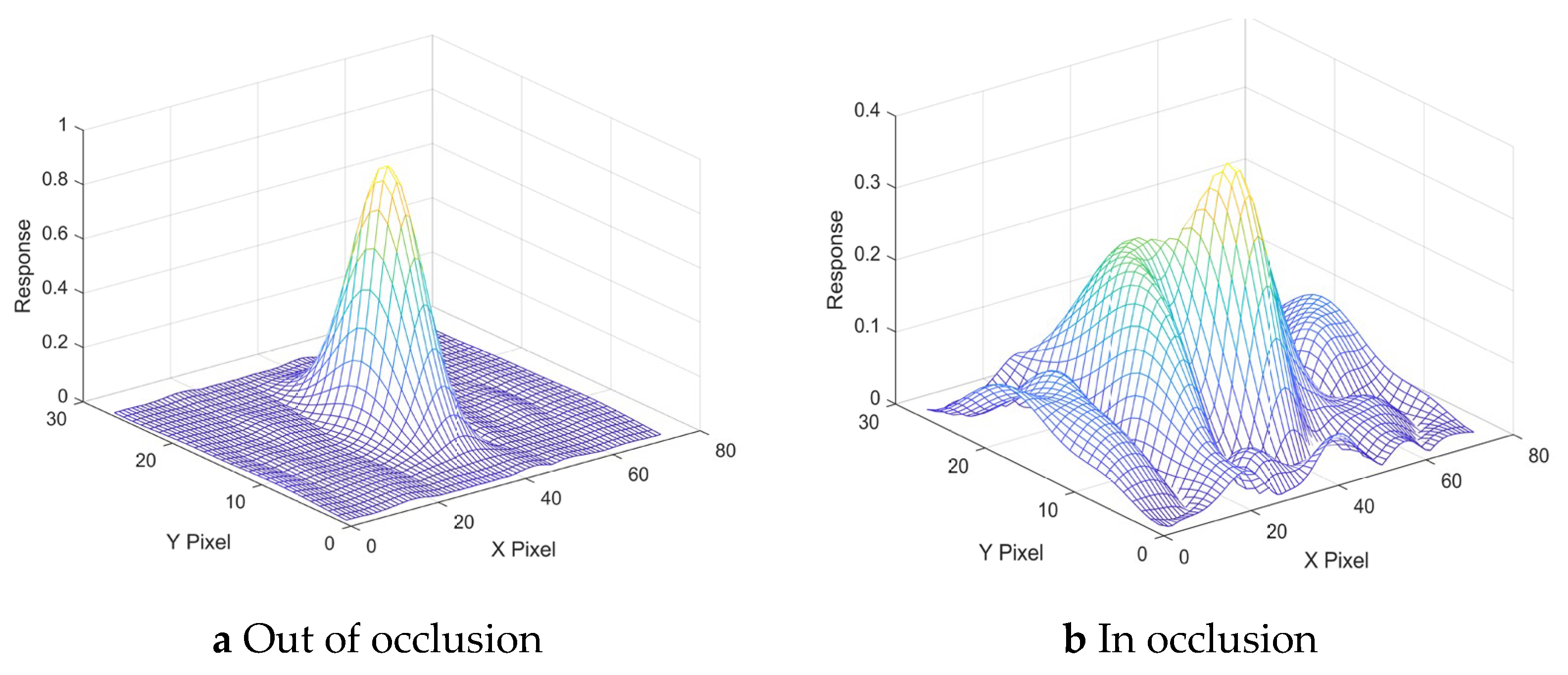
Aiming at the declining of tracking accuracy or even tracking failure when the target is in occlusion, this method uses the peak sidelobe ratio (PSLR) and intrinsic shape signature (ISS) to effectively judge the occlusion state of the target. Then, an adaptive factor is proposed to fuse the tracking results of kernel correlation filter and Kalman filter, according to the occlusion state of the target, improving the tracking accuracy when the target is in occlusion.

2. Intensity Image KCF Target Tracking Method Based on the Muti-Feature Fusion

KCF is a classical tracking model based on kernel function and correlation filtering theory. By expanding training samples through cyclic matrix, discriminant classifier is trained to judge the target, achieving rapid detection and recognition of the target [16].

The main process is as follows:

Step 1: The HOG feature of the target is extracted from the first frame for training and learning to build the correlation filter.

Step 2: The target position of the previous frame is taken as the search area, of which features are extracted. The edge effect is reduced by cosine window function, and the response map in frequency domain is obtained by fast Fourier transform.

Step 3: By implementing the inverse Fourier transform to generate the response map in time domain, the max peak position in this response map is the optimal target prediction position of the next frame.

Step 4: The HOG features of the target are extracted from the current frame, which are used for training and learning together with the expected output, while the correlation filter is updated.

Step 5: Repeat Step 2 to Step 4 to achieve continuous target tracking.

The overall flow of the KCF algorithm is shown in the figure below. ⊙ in Figure 1 means the multiplication of two outcomes in the frequency domain.

However, the HOG feature alone cannot fully describe the target, especially when the target is partially obscured or the image quality is blurred due to rain, snow and other environmental factors, which is prone to problems such as reduced tracking accuracy and even tracking failure. In order to overcome this shortcoming of KCF algorithm, this paper adopts multi-feature fusion method to fuse HOG feature and Fourier descriptor feature of target in LiDAR intensity image to improve tracking accuracy. The overall flow of the improved algorithm is shown in the figure below. ⊙ in Figure 2 means the multiplication of two outcomes in the frequency domain.

2.1. The Principle of KCF Tracking Algorithm

2.1.1. Ridge Regression

Ridge regression is a linear regression method with biased estimation, which is essentially an improved least square method [17]. By giving up the unbiasedness of the least square method, it is a regression method with more realistic regression coefficients obtained at the cost of reducing the accuracy, of which the fitting of ill-conditioned data is better than the least square method.

Suppose there is a training set $\left\{\left(a_1,b_1\right),\cdots \left(a_i,b_i\right)\right\}$ and a response function $f\left(a_i\right)=w^T{a}_i$. In order to minimize the mean square error between the response function of the sample vector $a_i$ and its corresponding label $b_i$, an optimization model about w is constructed as follows:

$$\begin{array}{c}w=\underset{w}{\arg \min }{\displaystyle \sum _i\left(f\left(a_i\right)-b_i\right)}+\lambda {\Vert w\Vert }^2\\ =\underset{w}{\arg \min }{\displaystyle \sum _i\left(w^T{a}_i-b_i\right)}+\lambda {\Vert w\Vert }^2\end{array}$$

(1)

where $\lambda$ is the regularization parameter that prevents overfitting; $w$ is weight coefficients expressed as a column vector; ${\Vert w\Vert }^2$ represents the 2-norm of $w$. Equation (1) has a unique optimal solution, which can be calculated by the following equation:

$$w={\left(A^{T}A+\lambda I\right)}^{-1}{A}^{T}b$$

(2)

Pluralize Equation (2) as follows:

$$w={\left(A^{H}A+\lambda I\right)}^{-1}{A}^{H}b$$

(3)

where $A$ represents a cyclic matrix consisting of cyclic shifts of the sample vector $a$; $I$ is a unit matrix; $A^H$ is the Hermite transpose of $A$.

2.1.2. Kernelized Correlation Detection

In practical scenarios, there are instances where the sample is not linearly separable in the low-dimensional space, necessitating the utilization of the “kernel trick” to map the sample into a higher-dimensional space for achieving linear separability. Assuming the availability of training sample set $X={\left[x_1,x_2,\cdots ,x_n\right]}^T$ and its corresponding label set $Y={\left[y_1,y_2,\cdots ,y_n\right]}^T$, we can formulate an optimization model for $w$ as follows:

$$w=\underset{w}{\arg \min }{\displaystyle \sum _i{\left(\langle w,\phi \left(x_i\right)\rangle -y_i\right)}^2}+\lambda {\Vert w\Vert }^2$$

(4)

where $\phi (·)$ represents the mapping from the original space to the Hilbert feature space, defined by the kernel function $\kappa (x,x^{\prime })=\langle \phi (x),\phi (x^{\prime })\rangle$. $x$ is the training sample, $x^{\prime }$ is the sample to be detected; based on the idea of “kernel technique”, the optimization model for $w$ can be expressed as a linear combination of inputs:

$$w={\displaystyle \sum _i{\alpha }_i\phi \left(x_i\right)}$$

(5)

In this case, the optimal solution of $w$ is the corresponding optimal solution $\alpha$ in Hilbert feature space. Therefore, the response function $f(z)$ can be expressed as:

$$\begin{array}{cc}f\left(z\right)& =w^T\phi \left(z\right)\hfill \\ & ={\displaystyle \sum _i{\alpha }_i}{\phi }^T\left(x_i\right)\phi \left(z_i\right)\hfill \\ & ={\displaystyle \sum _i{\alpha }_i\kappa \left(x_i,z_i\right)}\hfill \end{array}$$

(6)

where $z$ represents the patch to be detected with the same size as $x$ that is captured from the next frame during the tracking process. The closed solution of ridge regression based on “kernel technique” is as follows:

$$\alpha ={\left(K+\lambda I\right)}^{-1}y$$

(7)

where $K$, the Kernel matrix, can be expressed as follows:

$$K=C(k^{xx})$$

(8)

where $k^{xx}$ represents the kernel correlation between training sample $x$ and itself. By substituting the Equation (8) into the Equation (7), we can obtain:

$$F(\alpha )={\displaystyle \frac{F(y)}{F(k^{xx})+\lambda }}$$

(9)

The response value of patch $z$ can be obtained by the following equation:

$$\widehat{f}(z)=F^{-1}(F(k^{xz})\odot F(\alpha ))$$

(10)

where $k^{xz}$ represents the kernel correlation between training sample $x$ and patch $z$; $\odot$ stands for element-wise product; $F^{-1}$ is the inverse Fourier transform. Then the position corresponding to the maximum value of $\widehat{f}(z)$ is the optimal target prediction position.

2.2. KCF Tracking Algorithm Based on Muti-Feature Fusion

2.2.1. HOG Feature

HOG is a statistical method to calculate the local features of an image, which can effectively describe the local gradient information and edge distribution of the target [18]. The main calculation process is as follows:

Step 1: The tracking region image captured as input is converted into a binary image;

Step 2: The Gamma correction method was used to normalize the input image, as shown in Equation (11):

$$I\left(h_x,h_y\right)=I{\left(h_x,h_y\right)}^{Gamma}$$

(11)

where $I\left(h_x,h_y\right)$ is the image matrix, gamma = 5.0, generally.

Step 3: Calculate the oriental gradient information of pixels, as shown in Equations (12) and (13):

$$G_x\left(h_x,h_y\right)=I\left(h_{x+1},h_y\right)-I\left(h_{x-1},h_y\right)$$

(12)

$$G_y\left(h_x,h_y\right)=I\left(h_x,h_{y+1}\right)-I\left(h_x,h_{y-1}\right)$$

(13)

where $G_x\left(h_x,h_y\right)$ represents the horizonal gradient value; $G_y\left(h_x,h_y\right)$ represents the vertical gradient value. So, the gradient amplitude and direction of the image at $\left(h_x,h_y\right)$ can be expressed as:

$$G\left(h_x,h_y\right)=\sqrt{G_x{\left(h_x,h_y\right)}^2+G_y{\left(h_x,h_y\right)}^2}$$

(14)

$$\theta \left(h_x,h_y\right)={\tan }^{-1}\left({\displaystyle \frac{G_y\left(h_x,h_y\right)}{G_x\left(h_x,h_y\right)}}\right)$$

(15)

Step 4: The image is subdivided into many small cells and the gradient data for each cell is calculated. For each cell, its gradient orientation is divided into nine bins, and each bin is bounded by 20°. According to the gradient orientation, the gradient information of the cell is mapped to the corresponding bin.

Step 5: The gradient information in the block composed of cells is collected, and the HOGs in all blocks are connected in series to obtain the overall HOG feature.

2.2.2. Fourier Descriptor Feature

The Fourier descriptor is an example of the application of Fourier theory in shape analysis, whose basic idea is to describe the shape of the target in the frequency domain by using the Fourier transform of the target boundary curve [19]. The Fourier descriptor has invariance in translation, rotation and scale with an excellent performance in image classification.

The Fourier descriptor can be computed as follows:

Step 1: The tracking region image captured as input is converted into a binary image which will be normalized by the Gamma correction method.

Step 2: Canny edge detection algorithm is used to extract the contour point set $\left\{\left(x_i,y_i\right)|i=1,2,\cdots ,m\right\}$ of the target to be tracked;

Step 3: Calculate coordinates of the central point $\left(\overline{x},\overline{y}\right)$ of the contour:

$$\{\begin{array}{c}\overline{x}={\displaystyle \sum _{i=1}^m{x}_i}\\ \overline{y}={\displaystyle \sum _{i=1}^m{y}_i}\end{array}$$

(16)

Step 4: Convert a cartesian point to a polar point. Taking $\left(\overline{x},\overline{y}\right)$ as the pole of the polar coordinate system, the rectangular coordinate $\left\{\left(x_i,y_i\right)|i=1,2,\cdots ,m\right\}$ of the contour point is converted to the corresponding polar coordinate $\left\{\left(r_i,{\theta }_i\right)|i=1,2,\cdots ,m\right\}$.

$$\{\begin{array}{c}{r}_i=\sqrt{{\left(x_i-\overline{x}\right)}^2+{\left(y_i-\overline{y}\right)}^2}\\ {\theta }_i={\tan }^{-1}{\displaystyle \frac{y_i-\overline{y}}{x_i-\overline{x}}}\end{array}$$

(17)

where $r_i\left(i=1,2,\cdots ,m\right)$ is the distance from the contour point to the center point. $r_i\left(i=1,2,\cdots ,m\right)$ is sorted in ascending order to obtain the distance sequence from each contour point to the center point, denoted as $D=\left[r_1,r_2,\cdots ,r_m\right]$.

Step 5: The distance sequence is transformed by fast Fourier transform.

$$F\left(k\right)={\displaystyle \frac{1}{m}}{\displaystyle \sum _{i=0}^{m-1}D\left(i\right)}{e}^{-{\displaystyle \frac{j2\pi ik}{m}}}k=0,1,\cdots ,m-1$$

(18)

where after transformation, $F(0)$ in the boundary sequence represents the DC component, which cannot reflect the shape difference between different images. Therefore, we get rid of it and keep the rest. Finally, the Fourier descriptor is expressed as follows:

$$F_D=\left\{{\displaystyle \frac{F\left(2\right)}{F\left(1\right)}},{\displaystyle \frac{F\left(3\right)}{F\left(1\right)}},\cdots ,{\displaystyle \frac{F\left(m-1\right)}{F\left(1\right)}}\right\}$$

(19)

The Fourier descriptor is mainly based on frequency domain information and can capture periodic changes in images, while HOG feature mainly focuses on spatial gradient information. By fusing these two features, the frequency domain and spatial domain information can be comprehensively used to provide a more comprehensive target description. The Fourier descriptor has a certain robustness to the illumination change, because it represents the image through the frequency domain information. In a battlefield, lighting conditions can be constantly changing, and the introduction of the Fourier descriptor helps to reduce sensitivity to light. In this paper, serial fusion of HOG feature and the Fourier descriptor is implemented to improve the robustness of KCF tracking algorithm.

3. The Adaptive Fusion of KCF and Kalman Filter

The GM-APD LiDAR developed by our team can obtain the intensity image of the target through photon accumulation detection while acquiring the target point cloud. The intensity image can represent the surface reflectivity and shape of the target, and the point cloud can represent the distance and orientation of the target. Inspired by article [20], we propose an adaptive fusion method of point cloud tracking and intensity image tracking, combining the advantages of two different data sources to improve the tracking performance of GM-APD LiDAR. In addition, since the two kinds of images do not need to be calibrated jointly, the calculation speed of the algorithm is greatly improved. In this paper, the KCF tracking method based on multi-feature fusion is used to process the intensity image, while the Kalman filter tracking method is used to process the point cloud data, and finally the results of two methods are adaptive fused. Combining the advantages of the two methods, the proposed method has the advantages of high tracking speed and high tracking accuracy, and can avoid the situation of tracking accuracy decline or even tracking failure caused by target occlusion to a certain extent, improving the accuracy of tracking targets in different occlusion states effectively.

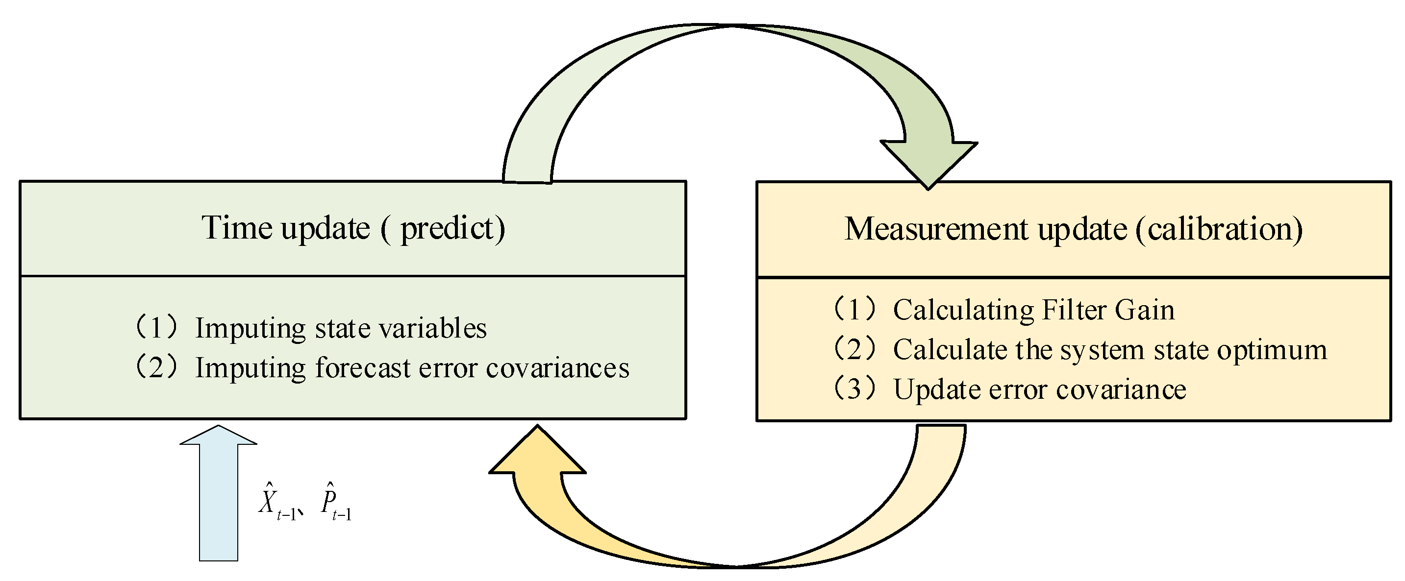
3.1. Target Tracking Method Based on Kalman Filter

Compared with correlation filtering algorithms, Kalman filter can predict the target position of the next frame by using information such as target velocity and acceleration, which can better estimate the state of random dynamic systems, achieving accurate target position prediction in the case of motion blur and occlusion [21]. Then, the point cloud target obtained by the KCF tracking algorithm is fused with the former one to form the target tracking results of each frame, enhancing the perceptual reliability. As a real-time recursive algorithm, Kalman filter models linear dynamic systems based on state transition equation and observation equation. The state transition equation is shown in Equation (20):

$$X_{\mathrm{t}}=A_t{X}_{t-1}+B_t{u}_t+{\omega }_t$$

(20)

where $X_t$ and $Z_t$ are the state of the system at time $t$ and the observation of that state, respectively; $A_t$ is a state transition matrix, which describes the transition process of the target from $X_{t-1}$ to state $X_t$; $u_t$ is a input variable; $B_t$ is a gating matrix, which controls $u_t$; ${\omega }_t$ is a process noise matrix, which is used to simulate the Gaussian distribution noise in the state transition process. The measurement equation is as follows:

$$Z_t=H_t{X}_{\mathrm{t}}+{\upsilon }_t$$

(21)

where $H_t$ is an observation matrix, where the elements represent the degree of influence of the system state variables on the observed variables; ${\upsilon }_t$ is the observation noise matrix exploited to simulate the Gaussian distribution noise in the observation process. Let the mean of $\omega$ and $\upsilon$ be 0 and the covariance be $Q$ and $R$, respectively, then their probability density distribution is:

$$\{\begin{array}{l}P\left(\omega \right)\sim N\left(0,Q\right)\\ P\left(\upsilon \right)\sim N\left(0,R\right)\end{array}$$

(22)

The Kalman filtering process is divided into two stages: prediction and update, as shown in Figure 3. In the prediction phase, the optimal estimation and state transition matrix of the target state of the previous moment are used to predict the target state of the current moment. Because the influence of the system noise is ignored in this stage, the predicted state will deviate from the actual state. In the update phase, the forecast state is adjusted by the observation data at the current time and the state observation matrix to obtain the optimal estimate of the target state [22].

Stage 1: Prediction

The state prediction of the target to be tracked at time $t$ is as follows:

$${\overline{X}}_{\mathrm{t}}=A_t{\widehat{X}}_{t-1}+{\omega }_t$$

(23)

$${\overline{P}}_t=A_t{\widehat{P}}_{t-1}{A}_t^T+Q_t$$

(24)

where ${\widehat{X}}_{t-1}$ is the optimal estimate of the target state at time $t-1$, ${\overline{X}}_{\mathrm{t}}$ is the prediction estimate at the current time, ${\widehat{P}}_{t-1}$ is the covariance matrix corresponding to the optimal estimate of the target state at time $t-1$, and ${\overline{P}}_t$ is the covariance matrix corresponding to the estimated value at the current time.

Stage 2: Update

Update the status of the target to be tracked at time $t$ as follows:

$$\{\begin{array}{l}{K}_t={\overline{P}}_t{H}_t^T{\left(H_t{\overline{P}}_t{H}_t^T+R_t\right)}^{-1}\\ {\widehat{X}}_t={\overline{X}}_t+K_t\left(Z_t-H_t{\overline{X}}_t\right)\\ {\widehat{P}}_t=\left(I_t-K_t{H}_t\right){\overline{P}}_t\end{array}$$

(25)

where $K_t$ is the Kalman gain matrix of the optimal estimation; $Z_t$ is the current observation value; $I_t$ is a unit matrix.

In the target tracking algorithm proposed in this paper, the target to be tracked is represented as a seven-dimensional vector $\left(x,y,z,\theta ,v_x,v_y,v_z\right)$, where $\left(x,y,z\right)$ represents the three-dimensional coordinates of the center point of the vehicle, respectively, $\left(v_x,v_y,v_z\right)$ represents the velocity components in the three directions during the driving process, respectively, and $\theta$ represents the direction of the vehicle.

Considering that the direction of the vehicle does not change significantly in the two adjacent point cloud images, the target angular velocity is ignored and a uniform motion model is adopted to describe the vehicle motion between adjacent point cloud sequences. The state of the vehicle target to be tracked is shown in Equation (26):

$$X={\left[x,y,z,\theta ,v_x,v_y,v_z\right]}^{\mathrm{T}}$$

(26)

According to the uniform motion model, the state $X_t$ at time $t$ is found, as shown in Equation (27):

$$X_t=\left[\begin{array}{ccccccc}1& 0& 0& 0& \Delta t& 0& 0\\ 0& 1& 0& 0& 0& \Delta t& 0\\ 0& 0& 1& 0& 0& 0& \Delta t\\ 0& 0& 0& 1& 0& 0& 0\\ 0& 0& 0& 0& 1& 0& 0\\ 0& 0& 0& 0& 0& 1& 0\\ 0& 0& 0& 0& 0& 0& 1\end{array}\right]\left[\begin{array}{c}{x}_{t-1}\\ y_{t-1}\\ z_{t-1}\\ {\theta }_{t-1}\\ v_{x_{t-1}}\\ v_{y_{t-1}}\\ v_{z_{t-1}}\end{array}\right]+\left[\begin{array}{c}{\omega }_x{}_{{}_{t-1}}\\ {\omega }_y{}_{{}_{t-1}}\\ {\omega }_z{}_{{}_{t-1}}\\ {\omega }_{\theta }{}_{{}_{t-1}}\\ {\omega }_{v_{x_{t-1}}}\\ {\omega }_{v_{y_{t-1}}}\\ {\omega }_{v_{z_{t-1}}}\end{array}\right]=A_t{X}_{t-1}+{\omega }_t$$

(27)

where $\Delta t$ is the time interval between two adjacent frames, $A_t$ is the state transition matrix from $X_{t-1}$ to $X_t$, and ${\omega }_t$ is the noise in the equation of motion and follows a zero-mean Gaussian distribution. Taking the output value of the model as the observed value of the state, the observation equation can be established, as shown in Equation (28):

$$Z_t=\left[\begin{array}{c}{x}_t\\ y_t\\ z_t\\ {\theta }_t\\ v_{x_t}\\ v_{y_t}\\ v_{z_t}\end{array}\right]=\left[\begin{array}{ccccccc}1& 0& 0& 0& 0& 0& 0\\ 0& 1& 0& 0& 0& 0& 0\\ 0& 0& 1& 0& 0& 0& 0\\ 0& 0& 0& 1& 0& 0& 0\\ 0& 0& 0& 0& 1& 0& 0\\ 0& 0& 0& 0& 0& 1& 0\\ 0& 0& 0& 0& 0& 0& 1\end{array}\right]\left[\begin{array}{c}{x}_t\\ y_t\\ z_t\\ {\theta }_t\\ v_{x_t}\\ v_{y_t}\\ v_{z_t}\end{array}\right]+\left[\begin{array}{c}{\upsilon }_{x_t}\\ {\upsilon }_{y_t}\\ {\upsilon }_{z_t}\\ {\upsilon }_{{\theta }_t}\\ {\upsilon }_{v_{x_t}}\\ {\upsilon }_{v_{y_t}}\\ {\upsilon }_{v_{z_t}}\end{array}\right]=H_t{X}_t+{\upsilon }_t$$

(28)

where $x_t$, $y_t$, $z_t$ are the 3D coordinates of the target centroid in the current frame, and ${\theta }_t$ is the vehicle driving direction angle. $v_{x_t}$, $v_{y_t}$, $v_{z_t}$ are the target velocity components in $x$, $y$, $z$ directions, respectively. And the velocity in a specific direction is determined by dividing the displacement between two consecutive frames in that direction by the time interval of those two frames.

3.2. Target Occlusion Judgment

Judging the occlusion state of the target at the current moment is the key to the effective fusion of the two algorithms. In this paper, PSLR [23] and ISS [24] are used to effectively judge the occlusion state of the target.

The PSLR is a physical quantity describing the degree of prominence of the main lobe relative to the sidelobe, which can be used to evaluate the matching degree of the two target signals of the related operation. It can be defined as:

$$PSLR={\displaystyle \frac{\max \left(f\left(z\right)\right)-\mu }{\sigma }}$$

(29)

where $\max \left(f(z)\right)$ is the response value of the main lobe; $\mu$ and $\sigma$ are the mean and variance of all sidelobes, respectively.

When the target is out of occlusion, the response graph has only the main lobe which is close to the ideal two-dimensional Gaussian distribution. When the target is in occlusion, multiple sidelobes appear in the response graph, and the contrast between sidelobe and peak value decreases, as shown in Figure 4:

The average PSLR value of the first five frames when the target is out of occlusion is taken as the standard response value ${\mu }_{PSLR}$, as shown in Equation (30). When the target is in full occlusion, the peak response is not 0. Through experimental tests, 0.3 ${\mu }_{PSLR}$ and 0.8 ${\mu }_{PSLR}$ are defined as the low and high threshold of the occlusion detection mechanism, respectively.

$${\mu }_{PSLR}={\displaystyle \frac{1}{5}}{\displaystyle \sum _{i=1}^{5}PSL{R}_i}$$

(30)

where $i$ is the image ordinal.

In the tracking process, the appearance characteristic information of the target is easy to change with the change of the scene. In order to adapt to the change of motion scene, the appearance model is adaptively updated with the PSLR.

$$\{\begin{array}{l}{\alpha }^i=\left(1-{\gamma }^i\right){\alpha }^{i-1}+{\gamma }^i{\alpha }^i\\ {\gamma }^i=\{\begin{array}{l}0 \hspace{1em}\hspace{1em}\hspace{1em}\hspace{1em}\hspace{1em}\hspace{1em}PSLR<T_L\\ {\displaystyle \frac{PSL{R}^i}{{\mu }_{PSLR}}}\times \beta \hspace{1em}otherwise\end{array}\end{array}$$

(31)

where $\alpha$ is the coefficient of the correlation filter, ${\gamma }^i$ is the adaptive parameter that varies with the PSLR value in each frame, and $\beta$ is a constant with the value of 0.025.

When the target is too close to the complex background or there is a texture similar to the target in the background, the response of the filter may be interfered by the background, which affects the accuracy of the PSLR. In order to enhance the robustness of the detection mechanism, the ISS detection algorithm is used to extract the key points of the point cloud target, and then the number of key points under different occlusion conditions is used as the evaluation criteria for occlusion state. The specific process is as follows:

Let the quantity of point cloud target be $N$, and the coordinate $p_i$ of any point is $\left(x_i,y_i,z_i\right)$.

Step 1: Set a search radius $r_f$ for each point $p_i$ of the point cloud;

Step 2: Calculate the weights $w_{ij}$ of each point $p_i$ within the radius $r_f$ of the point $p_i$:

$$\begin{array}{cc}{w}_{ij}={\displaystyle \frac{1}{|p_j-p_i|}}& ,|p_j-p_i|<r_f\end{array}$$

(32)

Step 3: Calculate the covariance matrix for point $p_i$:

$$\mathrm{cov}(p_i)={\displaystyle \frac{{\displaystyle \sum _{|pi-pj|<r_f}{w}_{ij}(p_j-p_i){(p_j-p_i)}^T}}{{\displaystyle \sum _{|pi-pj|<r_f}{w}_{ij}}}}$$

(33)

Step 4: Calculate all eigenvalues $({\lambda }_i^1,{\lambda }_i^2,{\lambda }_i^3)$ of the covariance matrix $\mathrm{cov}(p_i)$ in Step 3 and arrange them in descending order;

Step 5: Set threshold values ${\epsilon }_1$ and ${\epsilon }_2$, and the points satisfying Equation (34) are regarded as ISS feature points.

$$\{\begin{array}{c}{\displaystyle \frac{{\lambda }_i^2}{{\lambda }_i^1}}\le {\epsilon }_1\\ {\displaystyle \frac{{\lambda }_i^3}{{\lambda }_i^2}}\le {\epsilon }_2\end{array}$$

(34)

Step 6: Repeat all the steps above until you have traversed all the points.

Assuming that the number of key points extracted from the target point cloud at the moment before occlusion is $N$, 0.3 $N$ and 0.8 $N$ are defined as the low and high thresholds of the occlusion detection, respectively. The occlusion detection method is designed as follows:

$$\{\begin{array}{ll}\mathrm{no} \mathrm{occlusion}\hfill & 0.8\left({\mu }_{PSLR}+N_{iss}\right)\le \left(PSL{R}^i+N^i{}_{iss}\right)\hfill \\ \mathrm{partial} \mathrm{occlusion}\hfill & 0.3\left({\mu }_{PSLR}+N_{iss}\right)\le \left(PSL{R}^i+N^i{}_{iss}\right)\le 0.8\left({\mu }_{PSLR}+N_{iss}\right)\hfill \\ \mathrm{full} \mathrm{occlusion}\hfill & 0.3\left({\mu }_{PSLR}+N_{iss}\right)\ge \left(PSL{R}^i+N^i{}_{iss}\right)\hfill \end{array}$$

(35)

3.3. The Proposal of Adaptive Factor

According to the different occlusion conditions of the target, an adaptive factor $\epsilon$ is proposed, whose calculation formula is as follows:

$$\epsilon ={\displaystyle \frac{PSL{R}^i+N^i{}_{iss}}{{\mu }_{PSLR}+N_{iss}}}$$

(36)

The adaptive factor $\epsilon$ was used to modify the tracking results of KCF and Kalman filter, and the final tracking results were obtained:

$$\{\begin{array}{l}F\left(x,y\right)=\epsilon F_{KCF}\left(x,y\right)+\left(1-\epsilon \right)F_{KF}\left(x,y\right)\\ F_{op}\left(x,y,z\right)=F\left(x,y,F_{KF}\left(z\right)\right)\end{array}$$

(37)

where $F_{op}\left(x,y,z\right)$ is the optimal target estimation position combined with Kalman filter and KCF, $F_{KCF}\left(x,y,z\right)$ is the target position calculated by the KCF, and $F_{KF}\left(x,y,z\right)$ is the target position in the z direction calculated by the Kalman filter. It can be seen from the above equation that when the target is in an unobstructed state, $\epsilon$ pays more attention to the tracking result of the KCF. When the target is completely in occlusion, $\epsilon$ pays more attention to the tracking result of Kalman filter.

4. Experiment and Result Analysis

In order to verify the effectiveness of the proposed target tracking algorithm, MATLAB R2022a is used for experiment based on KITTI data set [25,26]. Then, GM-APD LiDAR data are used to verify the algorithm, and center location error (CLE) is used to evaluate the performance of the tracking algorithm. CLE refers to the Euclidean distance between the real target center position and the predicted target center position in the tracking process. The smaller the Euclidean distance, the higher the tracking accuracy. CLE calculation formula is as follows:

$$CLE=\sqrt{{\left(x_p-x_r\right)}^2+{\left(y_p-y_r\right)}^2+{\left(z_p-z_r\right)}^2}$$

(38)

where $p$ is the predicted target center location; $r$ is the real target center location; the KCF tracking algorithm uses a 4x4-sized grid to extract HOG feature, the histogram direction is 9, the sampling window size is 1.5 times of the initially selected region; the regularization parameter $\lambda ={10}^{-4}$, and the Gaussian Kernel bandwidth $\sigma =0.5$.

4.1. Tracking Experiment Based on KITTI Data Set

KITTI data set has given the relevant correction parameters for converting the camera coordinate system to the lidar coordinate system. Combining the rotation matrix $R$ and translation matrix $T$, the image tracking results can be associated with the LiDAR point cloud tracking results.

When using KITTI data set for tracking simulation, the color image is converted to a binary image to simulate the intensity image generated by GM-APD LiDAR. Then, KCF and Kalman filter are used to track the image and point cloud data, respectively. The tracking scene is KITTI data set tracking scene 0001, and the tracking target is No. 86 white car. The motion state sequence of the car from unshielded to blocked by other cars to unshielded is selected. When tracking the target, PSLR and ISS need to be calculated to judge the occlusion state of the target. Finally, according to the occlusion state, the adaptive factor is used to effectively fuse the intensity image with the point cloud to track the position information. The calculation results are shown in the figure below.

As can be seen from Figure 5, when the target is out of occlusion, the PSLR is 7.69 and the number of ISS key points is 9. When the target is partially obscured, the PSLR decreases to 5.62, and the number of ISS key points decreases to 6. When the target is in full occlusion, the PSLR is not 0 but drops to 1.77, and the number of ISS key points is 0. The results above all meet the threshold interval set in this paper when the target is completely occlusive, which proves that the occlusion threshold set in this paper is effective and meets the judgment of the subsequent tracking task on the target occlusion state. The tracking results are as shown partially in Figure 6:

In Figure 6, the red box is the real position of the target, and the yellow box is the tracking position of the algorithm. It can be seen that when the target is in the unobstructed state, the kernel correlation filtering based on multi-feature fusion can effectively track the target of interest; when the target is partially occlusive, the tracking results based on the multi-feature fusion kernel correlation filtering are biased. Kalman tracking algorithm can predict the target position with a small error, but the target motion state is not completely linear. Extended Kalman Filter (EKF) [27], based on Kalman filter, uses nonlinear functions to predict and estimate the state. By using the nonlinear function in the equation of state and the observed equation, and performing the Taylor series expansion of the nonlinear function, keeping only the first-order term, the nonlinear model is approximated to a linear model, so it is more accurate than the Kalman estimate. The tracking accuracy diagram was drawn for nine consecutive frames from No. 86 white car that was never occluded to that in occluded and then gradually out of occluded, as shown in Figure 7. By combining kernel correlation and Kalman tracker, the tracking accuracy is better than Kalman filter and EKF when the target is in the unobserved state. When the target is partially and completely occluded, the high tracking accuracy is still maintained through adaptive factor adjustment. As can be seen from

Table 1. Average CLE of different algorithms.

Algorithm	Kalman Filter	EKF	Proposed
Average CLE/m	0.1509	0.1284	0.1182
Average algorithm speed per frame/ms	34	45	51

, the average CLE of the proposed algorithm is 21.67% higher than that of Kalman filter and 7.94% higher than that of EKF, which proves that the proposed method can accurately track targets in different occlusion states.

4.2. Tracking Experiment Based on Data Collected by GM-APD LiDAR

Because the GM-APD LiDAR developed by our research group is limited by the number of arrays, the imaging of vehicles and other targets detected by close-range targets is incomplete. In this paper, we first conduct target tracking experiments with a fixed field of view for 285m distant pedestrian targets to ensure that complete target information can be obtained each time of imaging. In the same way, the original image with 64x64 resolution will be reconstructed with super resolution first and then the tracking experiment will be carried out. After the detection of the initial frame point cloud, the size information of the bounding box of the tracking target will be saved. For the next frame point cloud data, the predicted position of Kalman filter will be taken as the origin and the size of the bounding box will be 1.2 times. The detection scene of tracking experiment is shown in Figure 8. A total of 50 frames of data are continuously selected for the tracking experiment, and the tracking target position of each frame is manually marked. The tracking results of selected sequences are shown in Figure 9. The tracking accuracy diagram was drawn for six consecutive frames to show the performance in the no occlusion scenario, as shown in Figure 10. The estimation results of different algorithms are shown in

Table 2. Average CLE of different algorithms.

Algorithm	Kalman Filter	EKF	Proposed
Average CLE/m	0.1209	0.1084	0.0982
Average algorithm speed per frame/ms	16	24	33

.

As can be seen from the Figure 9 and Figure 10, the kernel correlation filtering tracking algorithm based on intensity image can track the target effectively because the target is not blocked, and the tracking algorithm after fusion can also track the target effectively. As can be seen from Table 2, the average CLE is 18.76% higher than Kalman filter, and the accuracy is 9.41% higher than EKF. Because the cloud data of the detection field is less than that of KITTI dataset, the average time per frame of the algorithm in this paper is 33 ms.

The target information in the above scenario is relatively complete. In order to further verify the performance of the proposed algorithm, the detection field of GM-APD LiDAR is fixed to detect and image the outdoor 600 m distant cross, and the point cloud data after the conversion of the intensity image and the range image generated by GM-APD LiDAR is followed up by tracking experiments. The target location of each scene is manually marked, and the detection scene is shown in Figure 11. The tracking results of selected sequences are shown in Figure 12. The tracking accuracy diagram was drawn for 14 consecutive frames to show the performance in the complex occlusion scenario, as shown in Figure 13. The estimation results of different algorithms are shown in

Table 3. Average CLE of different algorithms.

Algorithm	Kalman Filter	EKF	Proposed
Average CLE/m	0.2125	0.1797	0.1542
Average algorithm speed per frame/ms	18	27	39

.

As can be seen from Figure 12a, when the target is relatively complete in the intensity image, the kernel correlation filtering tracking algorithm can effectively track the target of interest. As the tracking target is blocked by the rear vehicle, as shown in Figure 12i, the tracking result based on the intensity image gradually fails, and the target position is predicted by Kalman filtering through adaptive factor adjustment. As can be seen from Table 3, the average CLE of the proposed algorithm in outdoor tracking scenes is 0.1542, which is 27.43% higher than that of Kalman filter and 14.19% higher than that of EKF. Because the detection data are affected by noise, the average processing time of each frame in this experiment is 39 ms.

5. Conclusions

In order to solve the problem of tracking accuracy decrease or even tracking failure due to target in occlusion, a target tracking method based on intensity image and point cloud data fusion is proposed in this paper. Firstly, the PSLR and ISS are used to effectively judge the occlusion state of the target. Then, an adaptive factor is proposed to fuse the tracking results of KCF and Kalman filter based on multi-feature fusion according to the different occlusion states of the target. Finally, accurate target location information is obtained. Based on KITTI data set, the proposed algorithm is verified by simulations. The average CLE of the proposed algorithm is 0.1182m, which is 21.67% better than that of Kalman filter, 7.94% better than that of EKF, and the average processing time per frame is 51 ms. Based on GM-APD LiDAR data, the proposed algorithm is verified by experiments. The average CLE of the proposed algorithm is 0.1262m, which is 23.1% better than that of Kalman filter algorithm and 8.68% better than that of EKF algorithm. The average processing time per frame is 36 ms. Both simulation and experimental results show that the proposed algorithm can greatly improve the tracking accuracy of targets in different occlusion states. In the future, we will consider validating the performance of the proposed methodology across a broader spectrum of scenarios, accounting for uncertainties arising from diverse environments including varying backgrounds, targets, lighting conditions, and obstacles. Simultaneously, we will conduct a more comprehensive categorization of occlusion situations and undertake an in-depth investigation into traffic congestion and high-density crowd scenarios.

References

1. Zhang, J.X.; Yang, G.H. Fault-tolerant output-constrained control of unknown Euler-Lagrange systems with prescribed tracking accuracy. Automatica 2020, 111, 108606. [Google Scholar] [CrossRef]
2. Giancola, S.; Zarzar, J.; Ghanem, B. Leveraging Shape Completion for 3D Siamese Tracking. In Proceedings of the IEEE/CVF Conference on Computer Vision and Pattern Recognition, Long Beach, CA, USA, 15–20 June 2019. [Google Scholar]
3. Zheng, C.; Yan, X.; Zhang, H.; Wang, B.; Cheng, S.; Cui, S.; Li, Z. Beyond 3D Siamese Tracking: A Motion-centric Paradigm for 3D Single Object Tracking in Point Clouds. In Proceedings of the IEEE/CVF Conference on Computer Vision and Pattern Recognition, New Orleans, LO, USA, 19 June 2022. [Google Scholar]
4. Xu, T.X.; Guo, Y.C.; Lai, Y.K.; Zhang, S.H. CXTrack: Improving 3D Point Cloud Tracking with Contextual Information. In Proceedings of the IEEE/CVF Conference on Computer Vision and Pattern Recognition, Vancouver, BC, Canada, 18–22 June 2023. [Google Scholar]
5. X.Z. Research on Single Target Tracking Technology Based on LiDAR Point Cloud. Ph.D. Thesis, National University of Defense Technology, Changsha, China, 1 December 2021.
6. T.D. Research on Target Detection and Tracking Technology in Complex Occlusion Environment. Ph.D. Thesis, Changchun University of Science and Technology, Changchun, China, 4 June 2021.
7. Bolme, D.S.; Beveridge, J.R.; Draper, B.A.; Lui, Y.M. Visual Object Tracking Using Adaptive Correlation Filters. In Proceedings of the 2010 IEEE Computer Society Conference on Computer Vision and Pattern Recognition, Washington, DC, USA, 13–18 June 2010. [Google Scholar]
8. Henriques, J.F.; Caseiro, R.; Martins, P.; Batista, J. Exploiting the Circulant Structure of Tracking-by-Detection with Kernels. In Proceedings of the 2012 European Conference on Computer Vision, Firenze, Italy, 7–13 October 2012. [Google Scholar]
9. Henriques, J.F.; Caseiro, R.; Martins, P.; Batista, J. High-Speed Tracking with Kernelized Correlation Filters. IEEE Trans. Pattern Anal. Mach. Intell. 2015, 37, 583–596. [Google Scholar] [CrossRef] [PubMed]
10. Hannuna, S.; Camplani, M.; Hall, J.; Mirmehdi, M.; Damen, D.; Burghardt, T.; Paiement, A.; Tao, L. DS-KCF: A Real-time Tracker for RGB-D Data. J. Real-Time Image Process. 2019, 16, 1439–1458. [Google Scholar] [CrossRef]
11. Zolfaghari, M.; Ghanei-Yakhdan, H.; Yazdi, M. Real-time Object Tracking based on an Adaptive Transition Model and Extended Kalman Filter to Handle Full Occlusion. Vis. Comput. 2020, 36, 701–715. [Google Scholar] [CrossRef]
12. Liu, Y.; Liao, Y.; Lin, C.; Jia, Y.; Li, Z.; Yang, X. Object Tracking in Satellite Videos based on Correlation Filter with Multi-Feature Fusion and Motion Trajectory Compensation. Remote Sens. 2022, 14, 777. [Google Scholar] [CrossRef]
13. Maharani, D.A.; Machbub, C.; Yulianti, L.; Rusmin, P.H. Deep Features Fusion for KCF-based Moving Object Tracking. J. Big Data 2023, 10, 136. [Google Scholar] [CrossRef]
14. Panahi, R.; Gholampour, I.; Jamzad, M. Real time occlusion handling using Kalman Filter and mean-shift. In Proceedings of the 2013 8th Iranian Conference on Machine Vision and Image Processing (MVIP), Zanjan, Iran, 10–12 September 2013. [Google Scholar]
15. Jeong, J.-M.; Yoon, T.-S.; Park, J.-B. Kalman filter based multiple objects detection-tracking algorithm robust to occlusion. In Proceedings of the SICE Annual Conference (SICE), Sapporo, Japan, 9–12 September 2014. [Google Scholar]
16. Feng, Z.; Wang, P. A model adaptive updating kernel correlation filter tracker with deep CNN features. Eng. Appl. Artif. Intell. 2023, 123, 106250. [Google Scholar] [CrossRef]
17. Sharma, U.; Gupta, N.; Verma, M. Prediction of compressive strength of GGBFS and Flyash-based geopolymer composite by linear regression, lasso regression, and ridge regression. Asian J. Civ. Eng. 2023, 24, 3399–3411. [Google Scholar] [CrossRef]
18. Jing, Q.; Zhang, P.; Zhang, W.; Lei, W. An improved target tracking method based on extraction of corner points. In The Visual Computer; Springer: Berlin/Heidelberg, Germany, 2024; pp. 1–20. [Google Scholar] [CrossRef]
19. S.Y. Research on Human Posture Recognition based on Infrared Image. Ph.D. Thesis, Shenyang Aerospace University, Shenyang, China, 8 March 2019.
20. Yan, H.; Zhang, J.X.; Zhang, X. Injected infrared and visible image fusion via L1 decomposition model and guided filtering. IEEE Trans. Comput. Imaging 2022, 8, 162–173. [Google Scholar] [CrossRef]
21. Yuan, Y.; Chu, J.; Leng, L.; Miao, J.; Kim, B.G. A scale-adaptive object-tracking algorithm with occlusion detection. EURASIP J. Image Video Process. 2020, 2020, 1–15. [Google Scholar] [CrossRef]
22. H.W. Research on 3D Vehicle Target Detection and Tracking Algorithm in Traffic Scene based on LiDAR Point Cloud. Ph.D. Thesis, Chang’an University, Xi’an, China, 29 April 2022.
23. Cui, Y.; Ren, H. Research on Visual Tracking Algorithm based on Peak Sidelobe Ratio. IEEE Access 2021, 9, 105318–105326. [Google Scholar] [CrossRef]
24. Zhong, Y. Intrinsic Shape Signatures: A Shape Descriptor for 3D Object Recognition. In Proceedings of the 2009 IEEE 12th International Conference on Computer Vision Workshops, Kyoto, Japan, 29 September–2 October 2009. [Google Scholar]
25. Zhang, J.X.; Yang, T.; Chai, T. Neural network control of underactuated surface vehicles with prescribed trajectory tracking performance. IEEE Trans. Neural Netw. Learn. Syst. 2022, 35, 8026–8039. [Google Scholar] [CrossRef] [PubMed]
26. Zhang, J.X.; Xu, K.D.; Wang, Q.G. Prescribed performance tracking control of time-delay nonlinear systems with output constraints. IEEE/CAA J. Autom. Sin. 2023, 11, 1557–1565. [Google Scholar] [CrossRef]
27. Ramadan, H.S.; Becherif, M.; Claude, F. Extended Kalman Filter for Accurate State of Charge Estimation of Lithium-based Batteries: A Comparative Analysis. Int. J. Hydrogen Energy 2017, 42, 29033–29046. [Google Scholar] [CrossRef]
Figure 1. Overall flow of KCF.
Applsci 14 07884 g001
Figure 2. Overall flow of KCF based on multi-feature fusion.
Applsci 14 07884 g002
Figure 3. The Kalman filtering process.
Applsci 14 07884 g003
Figure 4. 2D target response graph.
Applsci 14 07884 g004
Figure 5. The results of PSLR and ISS in different occlusion.
Applsci 14 07884 g005
Figure 6. The comparation of different methods in different occlusion.
Applsci 14 07884 g006aApplsci 14 07884 g006b
Figure 7. CLE curve of different algorithms in the tracking experiment based on KITTI data set.
Applsci 14 07884 g007
Figure 8. The first outdoor detection scenario.
Applsci 14 07884 g008
Figure 9. Tracking results of the first outdoor detection scenario.
Applsci 14 07884 g009aApplsci 14 07884 g009b
Figure 10. CLE curve of different algorithms in the first outdoor detection scenario.
Applsci 14 07884 g010
Figure 11. The second outdoor detection scenario.
Applsci 14 07884 g011
Figure 12. Tracking results of the second outdoor detection scenario.
Applsci 14 07884 g012aApplsci 14 07884 g012b
Figure 13. CLE curve of different algorithms in the second outdoor detection scenario.
Applsci 14 07884 g013