Abstract
A hysteretic model is essential for the study of the seismic performance of structures. Due to the ability to capture the component strength and stiffness deterioration, the modified Ibarra–Medina–Krawinkler (ModIMK) hysteretic model has been widely used recently. Previous studies on the ModIMK model have mainly focused on reinforced-concrete (RC) square columns, and very few have focused on circular columns. In contrast, studies on the ModIMK model specifically for corroded circular RC columns have not yet been conducted. For this reason, a database of 35 corroded and uncorroded comparison columns was gathered, and the hysteretic model parameters of each column were calibrated. The ratios of the model parameters of the corroded and uncorroded comparison components are defined as the corrosion-induced deterioration coefficients (CIDCs). After the CIDCs were calculated for all the corroded columns, the empirical equations for the CIDCs were established using regression methods. Through determining the ModIMK model parameters of the corroded columns when they were uncorroded, combined with these equations, the ModIMK model parameters of the corroded circular columns were calculated and their hysteretic models defined. Finally, the accuracy of the ModIMK model’s prediction method was demonstrated using the hysteretic response analyses of four components in the database and the application of two components outside the database. The prediction method lays the foundation for applying the ModIMK model to structures containing corroded circular RC columns.
1. Introduction
A hysteretic model capable of capturing structural component deterioration is required for the study of the seismic performance of structures. The Ibarra–Medina–Krawinkler (IMK) plastic hinge model was initially introduced by Ibarra et al. [1] Lignos et al. [2] proposed the modified IMK (ModIMK) model to address asymmetric component hysteretic behavior. Compared to alternative models [3], it is extensively utilized due to its good ability to efficiently simulate hysteretic characteristics.
Nonlinear analytical models for reinforced concrete components under earthquake ground motions are usually based on either “mechanics” or “phenomenological” laws [4,5,6,7]. The most typical mechanics-based model is the fiber model, the accuracy of which depends mainly on the definition of the constitutive laws of concrete and steel. In the case of serious damage, the deterioration in the component performance is associated with phenomena such as concrete crushing, reinforcement buckling, fracture, or slippage, and it is difficult to simulate the deterioration in the component performance in the fiber model due to the complex interaction of the geometric and material properties. The ModIMK model, on the other hand, is based on “phenomenological” laws, which describe the nonlinear behavior of the component in a simple moment–rotation form; the deterioration in the component’s performance can be empirically simulated based on statistical analysis of a large amount of test data, and its computational speed is much faster than the fiber model. Due to its superiority, the ModIMK model is recommended by ASCE 41.
By calibrating the model parameters of the components and subsequently regressing to derive the empirical equations for the model parameters, it is possible to make relatively accurate predictions regarding the hysteretic models of similar components [8,9,10]. Based on a test database for reinforced-concrete (RC) square columns failing in flexural or combined flexure–shear mode, Haselton et al. [11] calibrated the IMK model’s parameters and derived the empirical equations for the model parameters. Lignos et al. [12,13] created a database of steel and RC structural columns, modified the IMK model, and obtained prediction equations for the model parameters. Dai et al. [14] gathered test data for corroded RC square columns, performed a calibration study for the ModIMK model parameters, and established model parameter prediction equation for corroded columns. Dai et al. [15] developed a database of corroded concrete columns retrofitted with FRP (fiber-reinforced polymer) and determined its ModIMK model.
The research above focuses primarily on reinforced-concrete square columns, whereas circular columns, which are extensively utilized in the fields of building engineering and bridge engineering, have received relatively little attention. Dai et al. [16] collected test data for circular columns failing in flexural or combined flexure–shear mode, investigated the process for calibrating the parameters of the ModIMK model, and obtained prediction equations for each parameter. As for the calibration and prediction studies on the parameters of the ModIMK model for corroded circular columns, the authors of this work have not found any literature on the subject so far.
Therefore, 35 sets of test data related to corroded circular columns were collected [17,18,19,20,21,22,23,24,25,26]. After calibrating the model parameters for all the columns in the database, a set of empirical equations related to the model parameters was obtained using linear regression. Using this set of equations, a prediction method for the ModIMK hysteresis model was created. This prediction method allows the ModIMK hysteretic model to be applied to the seismic performance study of structures containing corroded circular RC columns.
2. Database
2.1. Collection of Test Data
The database was limited to 35 columns, due to the relatively low number of studies examining the hysteretic performance of corroded circular columns. Among these columns, 14 were uncorroded, and 21 were corroded. A more precise understanding of the corrosion rate’s impact on the hysteretic performance can be achieved by comparing the corroded columns to the uncorroded columns.
The primary considerations when gathering the experimental data included the following factors:
- (1)
- The corrosion area had to include the root of the corroded column, while columns that were corroded only in the middle were excluded from the collection.
- (2)
- All the design parameters of the corroded columns and the uncorroded comparative ones were identical, with the exception of the corrosion rate and the corrosion height ratio; corroded columns lacking comparative columns were not included in the collection.
- (3)
- The columns failed in flexural or combined flexure–shear mode; columns that failed in a shear mode were not included in the collection.
- (4)
- The cross-sectional shapes of the columns were circular; square columns were not included in the collection.
- (5)
- The transverse and longitudinal reinforcements were corroded at the same time, while the columns whose transverse reinforcements were not corroded were not included in the collection.
2.2. Design and Corrosion Parameters of the Columns
The analysis incorporated 17 design and corrosion parameters, the definitions of which are provided in Table 1. The following are the precise definitions of the two corrosion parameters:

Table 1.
Design and corrosion parameters of columns and their physical significance.
(1) Corrosion rate : the rate of corrosion in the longitudinal reinforcement, which is determined by dividing the average mass of the longitudinal reinforcement lost due to corrosion by the initial mass of the longitudinal reinforcement before corrosion.
(2) Corrosion height ratio : The parameter is calculated as the ratio of the height of the corroded section to the height of the column.
The value ranges of the primary design and corrosion parameters are shown in Table 2.
Table 2.
Ranges of important design and corrosion parameters.
2.3. Explanations of the Database
(1) The corrosion rates of the longitudinal reinforcement in columns 15, 17, and 19 were not provided in Zhou et al. [19]. Therefore, they were estimated according to the change in the longitudinal reinforcement elongation rate and the change in the chloride ion content of the surrounding concrete [27,28], and the average of the estimated values of the two methods was taken.
(2) In the case where the corrosion rate is not very high, the displacements of the two types of circular columns, which have the same corrosion rate in the plastic hinge area at the bottom and different corrosion rates in the part above the plastic hinge, are very close to each other in the small deformation stage under horizontal force [27]; while in the large deformation stage, the displacements of the column are mainly determined by the plastic hinge region [11]. Consequently, when various sections of the column exhibit varying corrosion rates, the corrosion rate of the column can be represented by the corrosion rate observed in the plastic hinge zone.
(3) The hysteretic curves obtained from the tests are represented in the form of horizontal shear versus horizontal displacement. However, in this work, these curves were converted to be described in terms of the bending moment and chord rotation, and the influence of the effect was considered during the conversion process [29].
(4) The type of static cyclic test configuration in this collection was cantilever [29].
(5) The columns failing in the shear failure mode were not collected in this paper because most of the corroded columns were not highly corroded, and most of them were in the flexural or flexural shear failure modes.
(6) The corrosion rate of the longitudinal reinforcement was used to represent the degree of corrosion in the column. Since the longitudinal reinforcement and the transverse reinforcement were corroded under the same conditions, and there was a strong correlation between the degree of corrosion of the two [14], the longitudinal reinforcement corrosion rate was chosen as an indicator to represent the degree of corrosion.
3. Hysteretic Model and Calibration of the Model Parameters for the Corroded Columns
3.1. Hysteretic Model
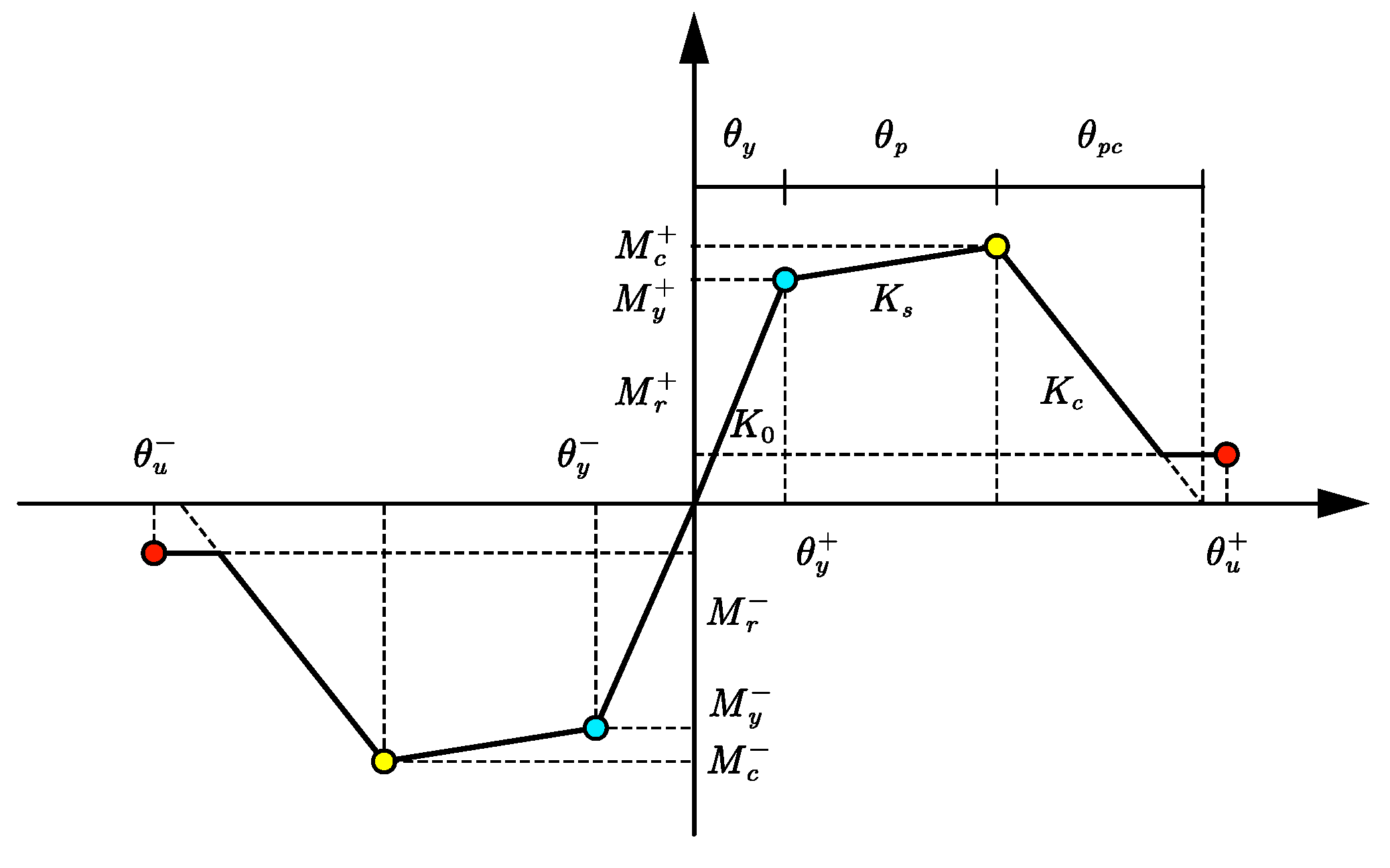
The backbone curve of the peak-oriented ModIMK hysteretic model is illustrated in Figure 1. The backbone curves, derived from the test results of the corroded columns and uncorroded comparative columns, are presented in Figure 2. It is evident that the components’ strength, stiffness, and ultimate deformation deteriorated due to corrosion. From Figure 2, we see that the ModIMK hysteresis model can be employed for both corroded and uncorroded columns, with the difference being that the hysteresis model for corroded columns needs to take into account the deterioration of each model parameter due to the corrosion.
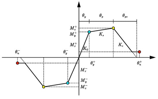
Figure 1.
The backbone curve of the ModIMK model.
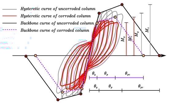
Figure 2.
The backbone curves of the corroded and uncorroded components.
The meaning of the primary model parameters is detailed in Table 3. For information on the remaining parameters, please consult the official OpenSees website or the relevant reference [2].
Table 3.
The parameters of the ModIMK model.
3.2. Calibration of the Model Parameters
Since the backbone curves of the ModIMK model are obtained through monotonic loading tests, but most of the components are not individually monotonically loaded, the hysteresis curves could not be used to calculate the parameters of the backbone curves directly. On the other hand, the deterioration in the strength and stiffness can only be assessed through an overall analysis of the hysteresis behavior of the components; so, the cyclic deterioration coefficients could not be obtained directly from the hysteresis curves either. Therefore, it was necessary to simulate the hysteresis curves of the test numerically. The hysteretic model parameters can be calibrated when the simulated and test hysteresis curves are well fitted.
For reinforced-concrete structures, a value of 0 is assigned to the residual moment ; four cyclic deterioration parameters, , are assumed to have an identical value, ; and a value of 1 is assigned to the exponent c [1,11]. Therefore, only six parameters are needed to determine the ModIMK hysteretic model: the five parameters associated with the skeleton curve, i.e., , and the parameters associated with the hysteresis rule, i.e., .
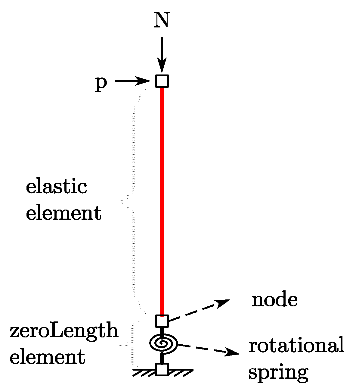
The OpenSees (3.3.0) software was utilized to establish the component analysis model, which is based on the ModIMK plastic hinge element (as illustrated in Figure 3). Since there is no plastic hinge before the component yields in a real experiment, in order to be equivalent to a fix-ended cantilever column, the stiffness of the plastic hinge and the elastic element in the analytical model must be adjusted before the yield strength is reached, i.e., the plastic hinge is tuned for high elastic stiffness, and the stiffness of the elastic element is adjusted accordingly [30,31,32].

Figure 3.
The analysis model using OpenSees.
The parameters of the ModIMK model were calibrated according to the methodology provided in Refs. [11,30]. The calibration process was conducted independently in the positive and negative loading directions. The mean values of the positive and negative calibration results are listed in Appendix Table A1.
4. Empirical Predictions of the Hysteretic Model Parameters for the Corroded Columns
4.1. Prediction Method
The procedures of the prediction methods consisted of the following steps:
(1) First, we calibrated the model parameters of the uncorroded comparative columns; if there was not an uncorroded comparative column, we predicted the model parameters, assuming that the corroded column was not corroded.
(2) Then, we calculated the corrosion-induced deterioration coefficients (CIDCs).
(3) Finally, the model parameters of the uncorroded columns were multiplied by the corresponding values of the CIDCs to forecast the corroded columns’ model parameters.
4.2. The Model Parameters in the Uncorroded State
There are two ways to determine the model parameters in the uncorroded state:
(1) When there is an uncorroded comparative column, which has identical design parameters to the corroded column, the model parameters of the uncorroded comparative column are calibrated. This was the case in this work when establishing the empirical regression equation.
(2) When there is not an uncorroded comparative column, one can predict the model parameters, assuming that the corroded column has not been corroded. Refer to Ref. [16] for these prediction methods. This approach is often required in practical engineering when applying the hysteretic model established in this work.
4.3. Empirical Regression Equations for the CIDCs
4.3.1. Corrosion-Induced Deterioration Coefficients
The corroded columns’ strength and stiffness deteriorated due to the corrosion. In order to quantify the effect of the corrosion on the model parameters, a corrosion-induced deterioration coefficient (CIDC) was defined. The coefficient is given by CIDC = , where and denote the model parameters of the corroded and uncorroded columns, respectively.
4.3.2. Illustration of the Regression Equations for the CIDCs
The CIDCs were estimated using the design and corrosion parameters of the corroded columns. The regression of the equations eliminated some outliers that appeared in the data due to the specific loading method of the test, experimental measurement errors, etc.
The stepwise linear regression method was used for regression, and parameters with a significance level of less than 0.05 were used as valid independent variables, determined through the t-test. Meanwhile, the problem of collinearity of the parameters used for regression was avoided by controlling the variance inflation factor (VIF) to be less than 10.
4.3.3. Regression Equations for the CIDCs
The hysteretic model parameters in the regression analysis were determined using the mean of the positive and negative calibration values.
A set of empirical equations was developed to relate the design and corrosion parameters of the columns (for details, refer to Appendix Table A2) to the CIDCs of the model parameters. They are in the following form:
For , the regression equation is not presented because there were relatively few columns where the capping points could be observed. We referred to the study of reinforced-concrete square columns in Ref. [11] to approximate the post-capping stiffness ; then, we calculated based on the already calibrated , i.e., Equation (6). According to Ref. [11], when obtains a large value, the loaded displacement is often not large enough to show the rapid deterioration in the stiffness; in fact, the stiffness deterioration is very fast when the loaded displacement is large. According to the 15 loaded columns with large displacement, the upper-limit value of was taken to be 0.1; with reference to this result, the upper limit value of was also taken to be 0.1 in this work.
The coefficients of determination (R2) for Equations (1)–(5) were 0.85, 0.79, 0.61, 0.81, and 0.61, respectively, which suggests that the fitting accuracy of the prediction equations was relatively high.
4.4. Predictions of Model Parameters for the Corroded Columns
The hysteretic model parameters for the corroded columns were predicted by multiplying the model parameters of the uncorroded columns by the corresponding values of the CIDCs.
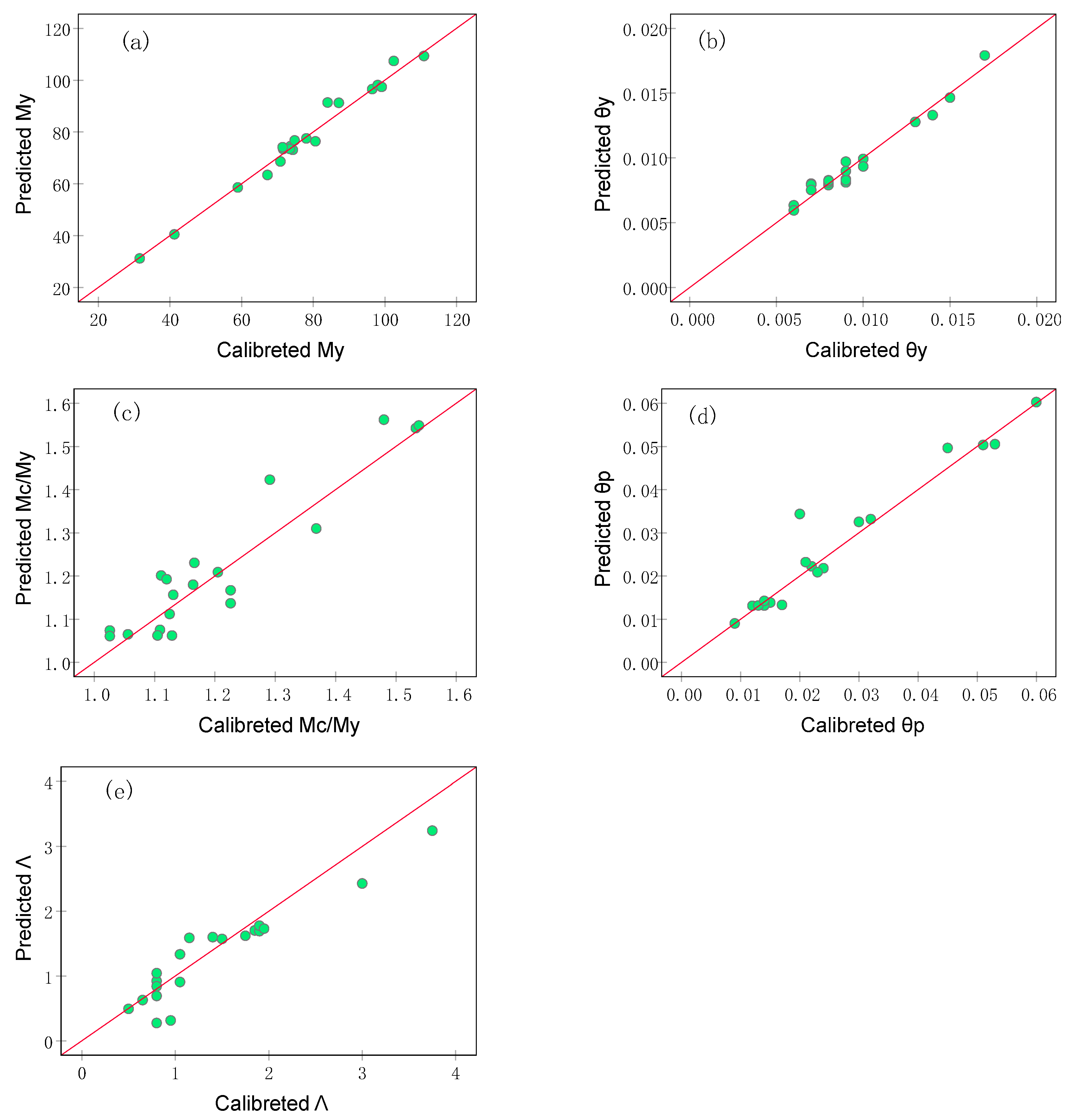
The calibrated and predicted model parameters for the corroded columns are illustrated in Figure 4, which shows that the proposed method provided good predictions of the model parameters for the corroded columns.
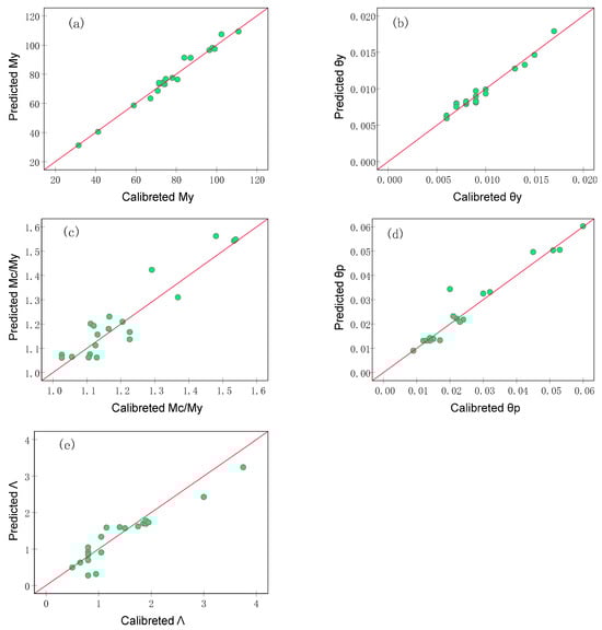
Figure 4.
Comparison between calibrated and predicted results of the model parameters. (a) ; (b) ; (c) ; (d) ; (e) .
Statistical comparisons among the ratios of the calibrated to the predicted values of the model parameters are presented in Table 4. The mean values of the ratios were 1.001, 0.996, 1.005, 1.006, and 1.016, corresponding to , respectively. The mean values were very close to 1, indicating that the prediction approach was accurate. The standard deviations for the ratios were 0.026, 0.032, 0.061, 0.066, and 0.166, corresponding to , respectively. None of these values indicate a significant dispersion, suggesting that the uncertainties for the prediction method were all relatively small.
Table 4.
Statistical comparison among the ratios of the calibrated to predicted values of the model parameters.
5. The Prediction Method’s Validation and Application
5.1. Validation within the Database
The degree of corrosion can be categorized into three types (less than 5% for slight corrosion, 5–10% for moderate corrosion, and more than 10% for high corrosion). Due to the small number of high-corrosion samples in the database established in this paper, the prediction method herein is more applicable to slight corrosion and moderate corrosion. For this reason, four randomly selected components in the database with slight and moderate corrosion were validated.
The test specimens C4-25, C9-40, CG10, and BX-1 were considered in the intra-database validation, and the design and corrosion parameters of all the specimens are documented in Appendix Table A2. The predicted values of the CIDCs and model parameters are presented in Table 5.
Table 5.
Predicted model parameters of the components in the database.
Comparing the predicted and the test hysteretic curves, as illustrated in Figure 5, we can see that the predicted curves were well fitted to the test curves. The yield and capping moments, as well as the loaded and unloaded stiffnesses, were predicted relatively accurately for each specimen; from specimens CG10 and BX-1, we can also see that the deteriorations were better predicted. Because the prediction equations were established through averaging the values of the positive and negative directions, and specimen C9-40 was asymmetric in the positive and negative directions, there was some error in the prediction of the model parameters.
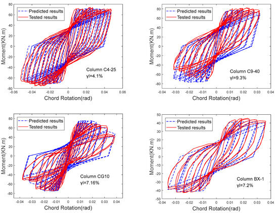
Figure 5.
Comparison between predicted and test results of the components in the database.
5.2. Extra-Database Application
Two random specimens with slight and moderate corrosion were considered for the extra-database application: specimen C9-25 from Ref. [17] and specimen C5 from Ref. [18]. The design and corrosion parameters of the two specimens are shown in Table 6. The predicted values of the CIDCs and model parameters are presented in Table 7.
Table 6.
Properties of the RC components for the extra-database application.
Table 7.
Predicted model parameters of the components for the extra-database application.
Upon comparing the predicted and test specimen hysteretic curves (refer to Figure 6), it is evident that the predicted curves also fit well with the test curves. The yield and capping moments, loaded and unloaded stiffnesses, and deteriorations were predicted relatively accurately for both specimens.
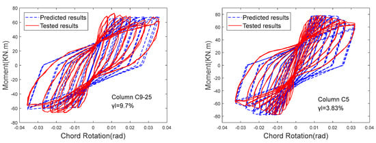
Figure 6.
Predicted and test results of the components for the extra-database application.
6. Summary and Conclusions
In this work, the prediction method of the ModIMK hysteretic model for corroded circular columns was investigated based on data statistics, and the main summary and conclusions are as follows:
(1) A database of 35 corroded and uncorroded comparative circular columns was established, and the ModIMK model parameters of all the components in the database were calibrated. The database was collected from published papers, and it was a good reference for the study of various properties of corroded circular RC columns.
(2) Empirical equations for CIDCs were established using linear regression. After the ModIMK model parameters of the corroded columns in the uncorroded state were determined and combined with these equations, the ModIMK hysteretic model of the corroded columns was defined. The method’s accuracy was demonstrated through hysteretic response analyses of six components.
(3) This study allowed the ModIMK hysteretic model to be applied to the seismic performance study of structures containing corroded circular RC columns, which could not be performed before. Due to the strength and stiffness deterioration-capturing capability of the ModIMK model, it was able to improve the reliability of the seismic analysis results as compared to other models, thus providing great help in seismic performance studies, seismic fragility studies, and seismic risk assessment of this type of structure.
The test data collected in this paper were limited, and the obtained prediction equations still have considerable room for improvement. As the research on corroded circular columns progresses and the relevant test data increase, the model can be revised continuously.
Author Contributions
Conceptualization, J.L. (Junqi Lin) and J.L. (Jinlong Liu); methodology, H.L.; software, H.L.; validation, H.L., J.L. (Junqi Lin) and J.L. (Jinlong Liu); formal analysis, H.L.; investigation, H.L.; resources, J.L. (Junqi Lin); data curation, H.L.; writing—original draft preparation, H.L.; writing—review and editing, H.L.; visualization, H.L.; supervision, J.L. (Junqi Lin); project administration, J.L. (Junqi Lin); funding acquisition, J.L. (Jinlong Liu). All authors have read and agreed to the published version of the manuscript.
Funding
This research was supported by “National Natural Science Foundation of China (U2239252)” and “The National Key Technology R&D Program (2012BAK15B05-04)”.
Data Availability Statement
The original contributions presented in the study are included in the article, further inquiries can be directed to the corresponding author.
Conflicts of Interest
The authors declare no conflict of interest.
Appendix A
Table A1.
Calibrated results of the model parameters.
Table A1.
Calibrated results of the model parameters.
| No. | Reference | Test No. | ||||||
|---|---|---|---|---|---|---|---|---|
| 1 | Ma [17] | c0-15 | 63.457 | 0.008 | 1.260 | 0.050 | — | 3.10 |
| 2 | c9-15 | 58.950 | 0.008 | 1.226 | 0.053 | — | 3.00 | |
| 3 | c0-25 | 71.414 | 0.009 | 1.254 | 0.050 | 0.076 | 3.80 | |
| 4 | c4-25 | 70.843 | 0.009 | 1.166 | 0.045 | — | 3.75 | |
| 5 | c0-40 | 85.005 | 0.007 | 1.173 | 0.041 | — | 1.70 | |
| 6 | c9-40 | 73.677 | 0.006 | 1.111 | 0.030 | 0.041 | 1.05 | |
| 7 | Zhu [18] | C0 | 79.200 | 0.009 | 1.094 | 0.013 | 0.094 | 2.00 |
| 8 | C5-40 | 74.809 | 0.008 | 1.109 | 0.015 | 0.129 | 1.85 | |
| 9 | C5-60 | 80.607 | 0.009 | 1.026 | 0.014 | 0.095 | 1.90 | |
| 10 | C10 | 71.602 | 0.008 | 1.129 | 0.014 | 0.139 | 1.40 | |
| 11 | C10-40 | 74.285 | 0.009 | 1.026 | 0.012 | 0.084 | 1.15 | |
| 12 | C10-60 | 73.500 | 0.009 | 1.105 | 0.013 | 0.107 | 1.40 | |
| 13 | CG10 | 71.464 | 0.008 | 1.056 | 0.017 | 0.088 | 1.75 | |
| 14 | Zhou [19] | LL | 36.132 | 0.011 | 1.701 | 0.055 | — | 1.95 |
| 15 | LLE | 31.581 | 0.009 | 1.480 | 0.060 | — | 1.90 | |
| 16 | MM | 73.913 | 0.018 | 1.532 | 0.094 | — | 2.70 | |
| 17 | MME | 67.228 | 0.015 | 1.291 | 0.048 | — | 1.95 | |
| 18 | MH | 106.514 | 0.022 | 1.463 | 0.081 | — | 4.15 | |
| 19 | MHE | 84.014 | 0.017 | 1.635 | 0.051 | — | 1.50 | |
| 20 | Li [20,21] | C80 | 96.212 | 0.012 | 1.183 | 0.031 | — | 0.75 |
| 21 | CC80 | 87.145 | 0.010 | 1.131 | 0.020 | — | 0.80 | |
| 22 | C140 | 86.405 | 0.008 | 1.213 | 0.009 | — | 0.45 | |
| 23 | CC140 | 78.073 | 0.006 | 1.368 | 0.009 | — | 0.50 | |
| 24 | Feng [22,23] | L0-N3-C0 | 104.436 | 0.010 | 1.409 | 0.023 | — | 0.90 |
| 25 | L0-N3-C360 | 96.466 | 0.007 | 1.533 | 0.024 | — | 1.05 | |
| 26 | C-L0-P20-N3 | 98.013 | 0.007 | 1.538 | 0.022 | — | 0.80 | |
| 27 | Aquino [24] | No.6 | 297.166 | 0.009 | 1.269 | 0.041 | 0.113 | 1.15 |
| 28 | No.4 | 275.996 | 0.007 | 1.120 | 0.013 | — | 0.80 | |
| 29 | Lao [25] | C-0-L0-N02 | 127.180 | 0.014 | 1.106 | 0.024 | — | 0.40 |
| 30 | C-10-L0-N02 | 102.470 | 0.013 | 1.226 | 0.021 | — | 0.95 | |
| 31 | C-20-L0-N02 | 99.102 | 0.014 | 1.125 | 0.023 | — | 0.80 | |
| 32 | C-0-L0-N04 | 135.747 | 0.011 | 1.067 | 0.018 | — | 0.80 | |
| 33 | C-10-L0-N04 | 110.905 | 0.010 | 1.164 | 0.014 | — | 0.65 | |
| 34 | Xie [26] | BW-1 | 44.895 | 0.010 | 1.176 | 0.029 | — | 0.75 |
| 35 | BX-1 | 41.254 | 0.009 | 1.205 | 0.032 | — | 0.80 |
Note: “—" denotes cannot be calibrated.
Table A2.
Values of the design and corrosion parameters.
Table A2.
Values of the design and corrosion parameters.
| No. | Test | d | c | L | s | λsp | ||||||||||||
|---|---|---|---|---|---|---|---|---|---|---|---|---|---|---|---|---|---|---|
| 1 | c0-15 | — | 1.000 | 260 | 30 | 820 | 32.400 | 16.0 | 0.023 | 373.20 | 572.30 | 100.0 | 8.0 | 0.010 | 327.00 | 6.250 | 3.154 | 0.150 |
| 2 | c9-15 | 9.50 | 1.000 | 260 | 30 | 820 | 32.400 | 16.0 | 0.023 | 373.20 | 572.30 | 100.0 | 8.0 | 0.010 | 327.00 | 6.250 | 3.154 | 0.150 |
| 3 | c0-25 | — | 1.000 | 260 | 30 | 820 | 32.400 | 16.0 | 0.023 | 373.20 | 572.30 | 100.0 | 8.0 | 0.010 | 327.00 | 6.250 | 3.154 | 0.250 |
| 4 | c4-25 | 4.10 | 1.000 | 260 | 30 | 820 | 32.400 | 16.0 | 0.023 | 373.20 | 572.30 | 100.0 | 8.0 | 0.010 | 327.00 | 6.250 | 3.154 | 0.250 |
| 5 | c0-40 | — | 1.000 | 260 | 30 | 820 | 32.400 | 16.0 | 0.023 | 373.20 | 572.30 | 100.0 | 8.0 | 0.010 | 327.00 | 6.250 | 3.154 | 0.400 |
| 6 | c9-40 | 9.30 | 1.000 | 260 | 30 | 820 | 32.400 | 16.0 | 0.023 | 373.20 | 572.30 | 100.0 | 8.0 | 0.010 | 327.00 | 6.250 | 3.154 | 0.400 |
| 7 | C0 | — | 0.455 | 300 | 30 | 1100 | 30.430 | 16.0 | 0.017 | 355.63 | 538.25 | 75.0 | 8.0 | 0.011 | 230.68 | 4.688 | 3.667 | 0.200 |
| 8 | C5-40 | 3.99 | 0.455 | 300 | 30 | 1100 | 30.430 | 16.0 | 0.017 | 355.63 | 538.25 | 75.0 | 8.0 | 0.011 | 230.68 | 4.688 | 3.667 | 0.200 |
| 9 | C5-60 | 4.45 | 0.455 | 300 | 30 | 1100 | 30.430 | 16.0 | 0.017 | 355.63 | 538.25 | 75.0 | 8.0 | 0.011 | 230.68 | 4.688 | 3.667 | 0.200 |
| 10 | C10 | 8.00 | 0.455 | 300 | 30 | 1100 | 30.430 | 16.0 | 0.017 | 355.63 | 538.25 | 75.0 | 8.0 | 0.011 | 230.68 | 4.688 | 3.667 | 0.200 |
| 11 | C10-40 | 8.41 | 0.455 | 300 | 30 | 1100 | 30.430 | 16.0 | 0.017 | 355.63 | 538.25 | 75.0 | 8.0 | 0.011 | 230.68 | 4.688 | 3.667 | 0.200 |
| 12 | C10-60 | 7.96 | 0.455 | 300 | 30 | 1100 | 30.430 | 16.0 | 0.017 | 355.63 | 538.25 | 75.0 | 8.0 | 0.011 | 230.68 | 4.688 | 3.667 | 0.200 |
| 13 | CG10 | 7.16 | 0.455 | 300 | 30 | 1100 | 30.430 | 16.0 | 0.017 | 355.63 | 538.25 | 75.0 | 8.0 | 0.011 | 230.68 | 4.688 | 3.667 | 0.200 |
| 14 | LL | — | 0.321 | 240 | 20 | 1400 | 40.000 | 12.0 | 0.015 | 400.00 | 540.00 | 50.0 | 6.0 | 0.011 | 400.00 | 4.167 | 5.833 | 0.057 |
| 15 | LLE | 10.50 | 0.321 | 240 | 20 | 1400 | 40.000 | 12.0 | 0.015 | 400.00 | 540.00 | 50.0 | 6.0 | 0.011 | 400.00 | 4.167 | 5.833 | 0.057 |
| 16 | MM | — | 0.250 | 240 | 20 | 1800 | 40.000 | 16.0 | 0.036 | 400.00 | 540.00 | 50.0 | 6.0 | 0.011 | 400.00 | 3.125 | 7.500 | 0.071 |
| 17 | MME | 10.50 | 0.250 | 240 | 20 | 1800 | 40.000 | 16.0 | 0.036 | 400.00 | 540.00 | 50.0 | 6.0 | 0.011 | 400.00 | 3.125 | 7.500 | 0.071 |
| 18 | MH | — | 0.250 | 240 | 20 | 1800 | 40.000 | 20.0 | 0.056 | 400.00 | 540.00 | 50.0 | 6.0 | 0.011 | 400.00 | 2.500 | 7.500 | 0.071 |
| 19 | MHE | 10.50 | 0.250 | 240 | 20 | 1800 | 40.000 | 20.0 | 0.056 | 400.00 | 540.00 | 50.0 | 6.0 | 0.011 | 400.00 | 2.500 | 7.500 | 0.071 |
| 20 | C80 | — | 0.857 | 300 | 30 | 1400 | 33.100 | 14.0 | 0.022 | 386.00 | 628.00 | 120.0 | 6.0 | 0.004 | 367.00 | 8.571 | 4.667 | 0.147 |
| 21 | CC80 | 5.10 | 0.857 | 300 | 30 | 1400 | 33.100 | 14.0 | 0.022 | 386.00 | 628.00 | 120.0 | 6.0 | 0.004 | 367.00 | 8.571 | 4.667 | 0.147 |
| 22 | C140 | — | 0.857 | 300 | 30 | 1400 | 33.100 | 14.0 | 0.022 | 386.00 | 628.00 | 210.0 | 6.0 | 0.002 | 367.00 | 15.000 | 4.667 | 0.410 |
| 23 | CC140 | 5.10 | 0.857 | 300 | 30 | 1400 | 33.100 | 14.0 | 0.022 | 386.00 | 628.00 | 210.0 | 6.0 | 0.002 | 367.00 | 15.000 | 4.667 | 0.410 |
| 24 | L0-N3-C0 | — | 0.900 | 300 | 30 | 1500 | 44.300 | 16.0 | 0.017 | 596.40 | 734.90 | 50.0 | 8.0 | 0.017 | 404.90 | 3.125 | 5.000 | 0.300 |
| 25 | L0-N3-C360 | 5.27 | 0.900 | 300 | 30 | 1500 | 44.300 | 16.0 | 0.017 | 596.40 | 734.90 | 50.0 | 8.0 | 0.017 | 404.90 | 3.125 | 5.000 | 0.300 |
| 26 | C-L0-P20-N3 | 3.82 | 0.900 | 300 | 30 | 1500 | 44.300 | 16.0 | 0.017 | 596.40 | 734.90 | 50.0 | 8.0 | 0.017 | 404.90 | 3.125 | 5.000 | 0.300 |
| 27 | No.6 | — | 0.571 | 500 | 25 | 2100 | 40.000 | 25.4 | 0.031 | 420.00 | 620.00 | 200.0 | 9.5 | 0.003 | 420.00 | 7.874 | 4.200 | 0.000 |
| 28 | No.4 | 4.00 | 0.571 | 500 | 25 | 2100 | 40.000 | 25.4 | 0.031 | 420.00 | 620.00 | 200.0 | 9.5 | 0.003 | 420.00 | 7.874 | 4.200 | 0.000 |
| 29 | C-0-L0-N02 | —— | 0.264 | 250 | 25 | 1135 | 32.700 | 16.0 | 0.025 | 458.00 | 620.00 | 100.0 | 8.0 | 0.010 | 454.00 | 6.250 | 4.540 | 0.200 |
| 30 | C-10-L0-N02 | 7.80 | 0.264 | 250 | 25 | 1135 | 32.700 | 16.0 | 0.025 | 458.00 | 620.00 | 100.0 | 8.0 | 0.010 | 454.00 | 6.250 | 4.540 | 0.200 |
| 31 | C-20-L0-N02 | 15.30 | 0.264 | 250 | 25 | 1135 | 32.700 | 16.0 | 0.025 | 458.00 | 620.00 | 100.0 | 8.0 | 0.010 | 454.00 | 6.250 | 4.540 | 0.200 |
| 32 | C-0-L0-N04 | —— | 0.264 | 250 | 25 | 1135 | 32.700 | 16.0 | 0.025 | 458.00 | 620.00 | 100.0 | 8.0 | 0.010 | 454.00 | 6.250 | 4.540 | 0.400 |
| 33 | C-10-L0-N04 | 7.80 | 0.264 | 250 | 25 | 1135 | 32.700 | 16.0 | 0.025 | 458.00 | 620.00 | 100.0 | 8.0 | 0.010 | 454.00 | 6.250 | 4.540 | 0.400 |
| 34 | BW-1 | —— | 0.286 | 240 | 25 | 1400 | 42.800 | 10.0 | 0.017 | 498.80 | 693.60 | 100.0 | 8.0 | 0.011 | 358.60 | 10.000 | 5.833 | 0.100 |
| 35 | BX-1 | 7.20 | 0.286 | 240 | 25 | 1400 | 42.800 | 10.0 | 0.017 | 498.80 | 693.60 | 100.0 | 8.0 | 0.011 | 358.60 | 10.000 | 5.833 | 0.100 |
Note: “—" in the column means “uncorroded”.
References
- Ibarra, L.F.; Medina, R.A.; Krawinkler, H. Hysteretic models that incorporate strength and stiffness deterioration. Earthq. Eng. Struct. Dyn. 2005, 34, 1489–1511. [Google Scholar] [CrossRef]
- Lignos, D.G.; Krawinkler, H. Deterioration modeling of steel components in support of collapse prediction of steel moment frames under earthquake loading. J. Struct. Eng. 2011, 137, 1291–1302. [Google Scholar] [CrossRef]
- Sivaselvan, M.V.; Reinhorn, A.M. Hysteretic models for deteriorating inelastic structures. J. Eng. Mech. 2000, 106, 633–640. [Google Scholar] [CrossRef]
- Terrenzi, M.; Spacone, E.; Camata, G. Comparison between phenomenological and fiber-section non-linear models. Front. Built Environ. 2020, 6, 38. [Google Scholar] [CrossRef]
- Zucca, M.; Reccia, E.; Longarini, N.; Eremeyev, V.; Crespi, P. On the structural behaviour of existing RC bridges subjected to corrosion effects: Numerical insight. Eng. Fail. Anal. 2023, 152, 107500. [Google Scholar] [CrossRef]
- De Domenico, D.; Messina, D.; Recupero, A. Seismic vulnerability assessment of reinforced concrete bridge piers with corroded bars. Struct. Concr. 2023, 24, 56–83. [Google Scholar] [CrossRef]
- Crespi, P.; Zucca, M.; Valente, M.; Longarini, N. Influence of corrosion effects on the seismic capacity of existing RC bridges. Eng. Fail. Anal. 2022, 140, 106546. [Google Scholar] [CrossRef]
- Wang, B.; Huo, G.; Sun, Y. Hysteretic behavior of steel reinforced concrete columns based on damage analysis. Appl. Sci. 2019, 9, 687. [Google Scholar] [CrossRef]
- Di Domenico, M.; Ricci, P.; Verderame, G.M. Empirical calibration of hysteretic parameters for modelling the seismic response of reinforced concrete columns with plain bars. Eng. Struct. 2021, 237, 112120. [Google Scholar] [CrossRef]
- Wei, K.; Xu, Y. Hysteretic model and parameter identification of RC bridge piers based on a new modified bouc-wen model. Structures 2022, 43, 1766–1777. [Google Scholar] [CrossRef]
- Haselton, C.B.; Liel, A.B.; Lange, S.T. Beam-Column Element Model Calibrated for Predicting Flexural Response Leading to Global Collapse of RC Frame Buildings; Pacific Earthquake Engineering Research Center: Berkeley, CA, USA, 2008. [Google Scholar]
- Lignos, D.G.; Krawinkler, H. Development and utilization of structural component databases for performance-based earthquake engineering. J. Struct. Eng. 2013, 139, 1382–1394. [Google Scholar] [CrossRef]
- Lignos, D.G. Sidesway Collapse of Deteriorating Structural Systems under Seismic Excitations. Ph.D. Thesis, Stanford University, Stanford, CA, USA, 2013. [Google Scholar]
- Dai, K.Y.; Yu, X.H.; Lu, D.G. Phenomenological hysteretic model for corroded RC columns. Eng. Struct. 2020, 210, 110315. [Google Scholar] [CrossRef]
- Dai, K.; Yu, X.; Jiang, Z.; Wang, D.; Qian, K. Hysteretic model for corroded reinforced concrete columns retrofitted with FRP. Constr. Build. Mater. 2023, 380, 131207. [Google Scholar] [CrossRef]
- Dai, K.Y.; Yu, X.H.; Wang, S. Identification of the hysteretic model parameters for reinforced concrete circular columns based on the modified ibarra-medina-krawinkler material model. Eng. Mech. 2021, 38, 154–163. (In Chinese) [Google Scholar]
- Ma, Y.; Che, Y.; Gong, J. Behavior of corrosion damaged circular reinforced conc-rete columns under cyclic loading. Constr. Build. Mater. 2012, 29, 548–556. [Google Scholar] [CrossRef]
- Zhu, J. Degradation of Capacity of the Corroded Reinforced Concrete Columns. Ph.D. Thesis, Shanghai Jiao Tong University, Shanghai, China, 2013. (In Chinese). [Google Scholar]
- Zhou, M.; Yin, S.; Zhu, G.; Fu, J. Seismic performance evaluation of highway bridges under scour and chloride ion corrosion. Appl. Sci. 2022, 12, 6680. [Google Scholar] [CrossRef]
- Li, J.; Li, Y. Experimental and theoretical study on the seismic performance of corroded RC circular columns strengthened with hybrid fiber reinforced polymers. Polym. Polym. Compos. 2014, 22, 653–660. [Google Scholar] [CrossRef]
- Li, J. Experimental and Theoretical Research on Hybrid FRP and Seismic Performance for Strengthening Corroded RC Columns. Ph.D. Thesis, Beijing University of Technology, Beijing, China, 2010. (In Chinese). [Google Scholar]
- Feng, R.; Li, Y.; Zhu, J.H.; Xing, F. Behavior of corroded circular RC columns strengthened by C-FRCM under cyclic loading. Eng. Struct. 2021, 226, 111311. [Google Scholar] [CrossRef]
- Liu, J.R. Research on the Seismic Behavior of Corroded RC Columns under the New Restoration System. Ph.D. Thesis, Harbin Institute of Technology, Harbin, China, 2019. (In Chinese). [Google Scholar]
- Aquino, W.; Hawkins, N.M. Seismic retrofitting of corroded reinforced concrete columns using carbon composites. ACI Struct. J. 2007, 104, 348–356. [Google Scholar]
- Lao, T.A. Experimental Study on Seismic Performance of Corroded Reinforced Concrete Columns under Large Strain FRP Confinement. Ph.D. Thesis, Shenzhen University, Shenzhen, China, 2010. (In Chinese). [Google Scholar]
- Xie, M.F. Seismic Behavior of Reinforced Concrete Piers with Basalt Fiber Sheets. Ph.D. Thesis, Shijiazhuang Tie Dao University, Shijiazhuang, China, 2020. (In Chinese). [Google Scholar]
- Li, Y.S. Time-Dependent Fragility Analysis of Reinforced Concrete Frame Structures under Chloride Environments at Coastal Areas of China. Ph.D. Thesis, Harbin Institute of Technology, Harbin, China, 2020. (In Chinese). [Google Scholar]
- Li, T.H.; Lin, J.Q.; Liu, J.L. Analysis of time-dependent seismic fragility of the offshore bridge under the action of scour and chloride ion corrosion. Structures 2020, 28, 1785–1801. [Google Scholar] [CrossRef]
- Berry, M.; Parrish, M.; Eberhard, M. Peer structural performance database user’s manual (version 1.0), 2004. Available online: https://nisee.berkeley.edu/spd/performance_database_manual_1-0.pdf (accessed on 6 August 2024).
- Haselton, C.B.; Liel, A.B.; Taylor-Lange, S.C.; Deierlein, G.G. Calibration of model to simulate response of reinforced concrete beam-columns to collapse. ACI Struct. J. 2016, 113, 1141–1152. [Google Scholar] [CrossRef]
- Ibarra, L.F.; Krawinkler, H. Global Collapse of Frame Structures under Seismic Excitations. Ph.D. Thesis, Stanford University, Stanford, CA, USA, 2004. [Google Scholar]
- Zareian, F.; Medina, R.A. A practical method for proper modeling of structural damping in inelastic plane structural systems. Comput. Struct. 2010, 88, 45–53. [Google Scholar] [CrossRef]


Disclaimer/Publisher’s Note: The statements, opinions and data contained in all publications are solely those of the individual author(s) and contributor(s) and not of MDPI and/or the editor(s). MDPI and/or the editor(s) disclaim responsibility for any injury to people or property resulting from any ideas, methods, instructions or products referred to in the content. |
© 2024 by the authors. Licensee MDPI, Basel, Switzerland. This article is an open access article distributed under the terms and conditions of the Creative Commons Attribution (CC BY) license (https://creativecommons.org/licenses/by/4.0/).