An Intelligent Real-Time Driver Activity Recognition System Using Spatio-Temporal Features

Abstract

With the rapid increase in the number of drivers, traffic accidents due to driver distraction is a major threat around the world. In this paper, we present a novel long-term recurrent convolutional network (LRCN) model for real-time driver activity recognition during both day- and nighttime conditions. Unlike existing works that use static input images and rely on major pre-processing measures, we employ a TimeDistributed convolutional neural network (TimeDis-CNN) layer to process a sequential input to learn the spatial and temporal information of the driver activity without requiring any major pre-processing effort. A pre-trained (CNN) layer is applied for robust initialization and extraction of the primary spatial features of the sequential image inputs. Then, a long short-term memory (LSTM) network is employed to recognize and synthesize the dynamical long-range temporal information of the driver’s activity. The proposed system is capable of detecting nine types of driver activities: driving, drinking, texting, smoking, talking, controlling, looking outside, head nodding, and fainting. For evaluation, we utilized a real vehicle environment and collected data from 35 participants, where 14 of the drivers were in real driving scenarios and the remaining in non-driving conditions. The proposed model achieved accuracies of 88.7% and 92.4% for the daytime and nighttime datasets, respectively. Moreover, the binary classifier’s accuracy in determining whether the driver is non-distracted or in a distracted state was 93.9% and 99.2% for the daytime and nighttime datasets, respectively. In addition, we deployed the proposed model on a Jetson Xavier embedded board and verified its effectiveness by conducting real-time predictions.

1. Introduction

1.1. Motivation

The dramatic worldwide increases in road traffic deaths and injuries have become a serious health and development concern around the world. Over a million people lose their lives as a result of traffic accidents, and as many as 50 million people are injured each year worldwide [1]. Currently, road traffic accidents are the leading cause of death for children and young adults. Researchers predict that between now and 2030, road traffic accidents will increase from being the ninth leading cause of death globally to the seventh [1]. According to the National Highway Traffic Safety Administration (NHTSA), approximately 60% of road traffic incidents occurred during the day, while more than 40% of all accidents occurred at night, despite less traffic. And driver distraction was a factor in 8% of fatal accidents and 15% of accidents resulting in injuries [2]. Several factors have been identified which affect the likelihood of road traffic accidents. Among them, driver distraction is one of the most prominent factors in road accidents. Driver distraction is any type of activity that draws driver attention away from safe driving during the day- and nighttime conditions. Dialing or talking on a cell phone, operating the navigation system, smoking, eating, and drinking while driving are a few examples of distracted driving [2]. In addition, nodding off to sleep, fainting, and mind wandering while driving lead to a relative disengagement from safe driving and are considered to be major contributors to fatal traffic accidents [3]. In general, driver distractions are categorized into three major classes, including visual distractions (taking eyes off the road), manual distractions (taking hands off the wheel), and cognitive distractions (taking the mind off of safe driving) [4]. Therefore, limiting the contributors to these risk factors is important to the success of efforts to reduce the severity of road accidents and injuries.

In this paper, a real-time driver behavior recognition system based on LRCN is proposed, which effectively detects driver activities in both day- and nighttime conditions. Figure 1 depicts the overview of the proposed system. A series of five consecutive images is used as an input to the LRCN model. The more generic name for LRCN is CNN-LSTM, corresponding to LSTM that uses a convolutional layer in the front end. A pre-trained CNN named Visual Geometry Group (VGG), a neural network with 16 layers, is applied to facilitate fast training by benefiting from transfer learning, where a trained model architecture and weights can be reused for a similar purpose. Then, each layer of the CNN is wrapped with a TimeDistributed (TimeDis) layer to maintain the temporal structure of the input data. Next, LSTM is integrated for end-to-end fine tuning as well as to learn the sequential input to decide the final driver state. The main motivation for selecting LRCN as a modeling approach is that driver actions appear in a sequence of images comprising spatial and temporal information which CNN alone fails to capture. In fact, a single CNN can detect these correlations, but it requires deep feature engineering such as background subtraction and other related segmentation techniques, which can be computationally expensive. Instead, LSTM is explicitly designed for sequence data to learn long-term dependencies. Thus, it is considered to capture and synthesize both the spatial and temporal features without any background subtraction efforts. Unlike existing studies, our approach works against nine different driver behaviors including non-distracted driving, drinking, controlling, smoking, texting, looking outside, talking with a passenger, head nodding, and fainting during both day- and nighttime in real-time conditions. During nighttime, due to the low intensity lighting conditions, RGB sensors alone are inadequate for accurately capturing drivers’ actions. Thus, due to the distinct natures of light during daytime and nighttime, a RGBDT sensor module is used to obtain the RGB and thermal infrared (IR) images separately during daytime and nighttime, respectively. To the best of our knowledge, this is the first system that considers both RGB color and IR images and employs an effective hybrid deep learning tool for robust real-time driver behavior recognition. Thus, it can be simply integrated into the design of an advanced driver assistance system (ADAS) to provide real-time warnings to drivers, reducing potential risks at any time of day.

1.2. Related Works

In the last few decades, detecting driver behaviors has become an active research theme. Various machine learning (ML) and deep learning (DL) techniques have evolved to recognize driver behavior. In more recent decades, many studies have focused on extracting driver body features such as eye gaze direction [5] and eye closure duration, head pose [6] or posture [7,8], hand cues [9], and gaze fixation time [10] to classify drivers’ distraction actions. These features have been widely used to identify driver sleepiness [11,12], driver fatigue [13,14], and driver drowsiness [15,16]. However, extracting gaze direction, the positions of hand and body joints, and head pose angles is not always easy to achieve and requires specific hardware devices, which leads to high computational costs [17].

Works utilizing machine learning models include Osman et al. [18], who used vehicle data such as acceleration, speed, and pedal positions to identify drivers’ engagement in secondary tasks, including cellphone calls and texting. The author reported that Decision Tree and Random Forest models performed best in detecting and classifying these tasks. Similarly, in 2019, Mousa et al. [19] used an Extreme Gradient Boosting (XGB) algorithm to identify factors leading to crashes and near-crash events. The XGB classifier was compared to three other ML algorithms, and driver behavior and intersections were identified as major crash contributors. Additionally, Bakhit et al. [20] implemented driver visual analysis using the driver eye glance frequency, glance duration, and glance eccentricity to distinguish crash and/or near-crash events from non-crash events. In addition, three subsequent studies used the naturalistic driving dataset (SHRP2) to investigate the causes of the crash and near-crash events associated with driver secondary tasks. The studies revealed driver actions including reaching for objects, reading, exceeding the speed limit, violations of stop signs, and improper turns as significant contributors to crash and near-crashes events [21,22,23]. In another study, Berri et al. [24] proposed the support vector machine (SVM) algorithm, which extracts the characteristic features of driver images to detect the use of cell phones while driving.

On the other hand, some of the works on deep learning include Yan et al. [25], who adopted a deep learning model, CNN, to analyze four driver activities based on the Southeast University (SEU) driving posture datasets. This dataset contains video clips covering four driving postures such as eating, safe driving, smoking, and answering mobile phones. Ahlstrom et al. [26] presented a context-dependent distracted driver detection algorithm, AttenD2.0, which was an extension of their original AttenD [5] algorithm that uses eye-tracking data. The authors used multiple time buffers to effectively keep track of how frequently and how long the driver’s eye is off the road ahead, thus identifying a distracted driver. In addition, a region convolutional neural network (RCNN) was proposed to classify driver activities such as using a cell phone, eating, braking, and operating the steering wheel [27]. During the experiment, skin-like regions of the images were first extracted using a Gaussian mixture model (GMM) method and then forwarded to RCNN to classify the final driver state. Majdi et al. [28] designed the Drive-Net architecture, which combines a CNN and a random decision forest to classify ten various driver distraction behaviors. In another study, Abouelnaga et al. [29] proposed an ensemble of various CNNs to classify ten distracted driver postures. The classifier model was trained using raw images as well as face and hand images to make the classification accuracy robust.

Furthermore, Zhang et al. [30] built a mock-up car environment equipped with front and side cameras to obtain multi-stream video data. This paper introduced an interwoven convolutional neural network (InterCNN) to detect different behaviors, including the use of a mobile device, eating, and drinking. Baheti et al. [31] adopted VGG-16 [32] architecture to detect nine different manual distraction activities and safe driving. In this experiment, the VGG-16 architecture was modified by employing various regularization methods such as dropout and ridge regression (L2) regularization while maintaining the overall classification accuracy. Furthermore, Tran et al. [33] designed a simulated driving testbed and utilized four different deep CNNs, including VGG-16 [32], AlexNet [34], GoogLeNet [35], and a residual network. Ten various driving activity datasets collected from the side view of the driver were considered, including normal and distracted driving postures. The authors reported that the GoogleNet approach achieved better detection performance compared to the other DCNNs implemented while testing on the designed driving simulator. Lastly, Xing et al. [17] investigated the impact of pre-trained architecture, namely AlexNet [34], GoogLeNet [35], and ResNet50 [36], to detect seven driver activities. A Kinect camera mounted on the front side of the driver was used to collect the raw RGB images of the driver activities. Then, prior to feeding the images to the classifier network, the raw images were first segmented using the GMM to extract the driver region from the background. The experiment reveals that applying the described segmentation system can significantly enhance the recognition accuracy.

Despite the substantial progress that has been achieved in the detection of driver behavior studies, there are still several problems that need to be addressed. In most existing works, particularly computer vision-based driver behavior studies have widely applied visible RGB images that limit the recognition model to only broad daylight or daytime. Thus, recognizing drivers’ behavior during nighttime conditions remains one of the main issues in the current computer vision-based driver activity recognition studies. Furthermore, previous studies utilized static input image information and employed various CNN variants along with significant traditional preprocessing measures such as background subtraction and image segmentation. These techniques can be time-consuming and increase computational costs. On the other hand, it is worth noting that some of the studies focused on limited types of driver distraction actions. Thus, our proposed work addresses the problem discussed.

1.3. Contribution

The main contributions of this paper can be summarized as follows.

• We develop a real-time end-to-end deep learning system that synergistically combines TimeDis-CNN and LSTM models to detect drivers’ behavioral patterns in real vehicle settings. Unlike prior studies that heavily depend on complex feature extraction, the proposed system does not require any major pre-processing steps and performs well in a complex and cluttered background environment with reduced computational cost. Moreover, nodding off to sleep and fainting while driving, which are considered to be two of the major leading causes of road traffic accidents, are studied.
• In contrast to most existing works, we also address nighttime recognition in addition to daytime. An important note is that, although the number of drivers decreases substantially at night, the number of traffic accidents occurring at night is significantly higher than during the daytime, and human errors and distractions are involved in most accidents. As such, this work considered thermal IR images to study the driver behavior during nighttime conditions.
• We collect naturalistic adequate datasets to effectively study driver activity and report a real-time implementation system for both day- and nighttime scenarios. The designed end-to-end LRCN model directly works on the raw sequential images received from the RGBDT sensor module and automatically extracts the optimal features to execute the final recognition and detection system.

2. Experiment Setup and Data Collection

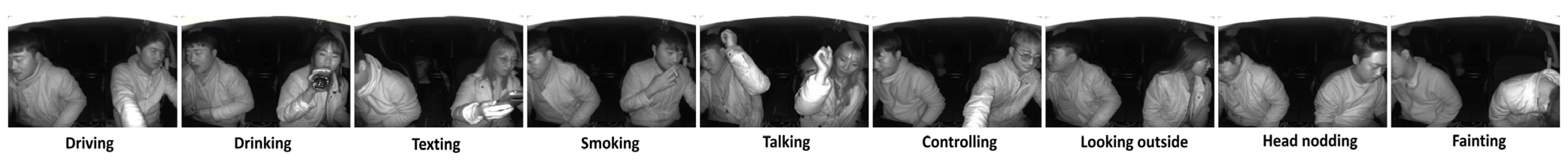
2.1. Data Collection

As shown in Figure 2, the data collection was carried out in a real vehicle cabin in collaboration with the Korea Automotive Technology Institute (KATECH) by using a well-equipped Hyundai Genesis G80 model car. A total of 31 participants were recruited (19 males, ages ranging between 25 and 44 years; and 12 females, ages ranging between 28 and 41 years). Among the participants, 10 drivers wore eyeglasses during the collection process. This allows the proposed model to recognize driver activities without any limitation of wearing eyeglasses. We particularly focused on nine driver behaviors that typically occur while driving and operating a vehicle.

• Non-distracted driving: driving with both hands on the wheel.
• Drinking: the participant drinking a plastic bottle while driving.
• Talking: the driver engages in conversation with the passenger by raising their right arm hand from the wheel.
• Controlling: when a driver is interacting with a navigation system, radio, and dashboard.
• Looking outside: looking completely outside in the left direction while driving.
• Texting: the participant manually dials or writes a text while driving.
• Smoking: smoking while driving.
• Head nodding: when the driver is nodding off to sleep.
• Fainting: corresponds to when the driver’s head and body are completely down.

The collection process was conducted in two subsequent phases. In the first phase, 14 drivers were involved in real driving conditions and requested to perform the pre-defined actions. However, head nodding and fainting actions in a real driving scenario may cause an unexpected accident. Thus, it was excluded from the first collection process. In this collection process, only RGB color images were obtained for all of the participants at several different times. In contrast, in the second collection phase, another 17 drivers were recruited to perform all of the pre-defined actions including the head nodding and fainting activities in non-driving conditions, and both RGB color images and IR images were collected at the same time. IR images only sense differences of heat within a temperature range, so instead of color or geometry, it includes the temperature information and eliminates the typical illumination problems which occur in RGB images [37].

Moreover, the IR images enable the proposed system to study the driver’s activity during nighttime conditions, which is disregarded in most similar existing works. Around 60 thousand and 20 thousand image frames were collected for RGB and IR images, respectively. Figure 3 and Figure 4 show overviews of the data samples collected for RGB and IR images, respectively. For each driver, a video dataset was obtained using a RGBDT sensor mounted on the front to capture the whole head and body movement with a resolution of 1280 × 720 and 640 × 480 for the RGB and IR images, respectively. The video recorded using the sensor was then routinely sectioned into a sequence of image frames. Then, data labeling was performed by first creating an action category for each driver and manually labeling each image according to the pre-defined categories.

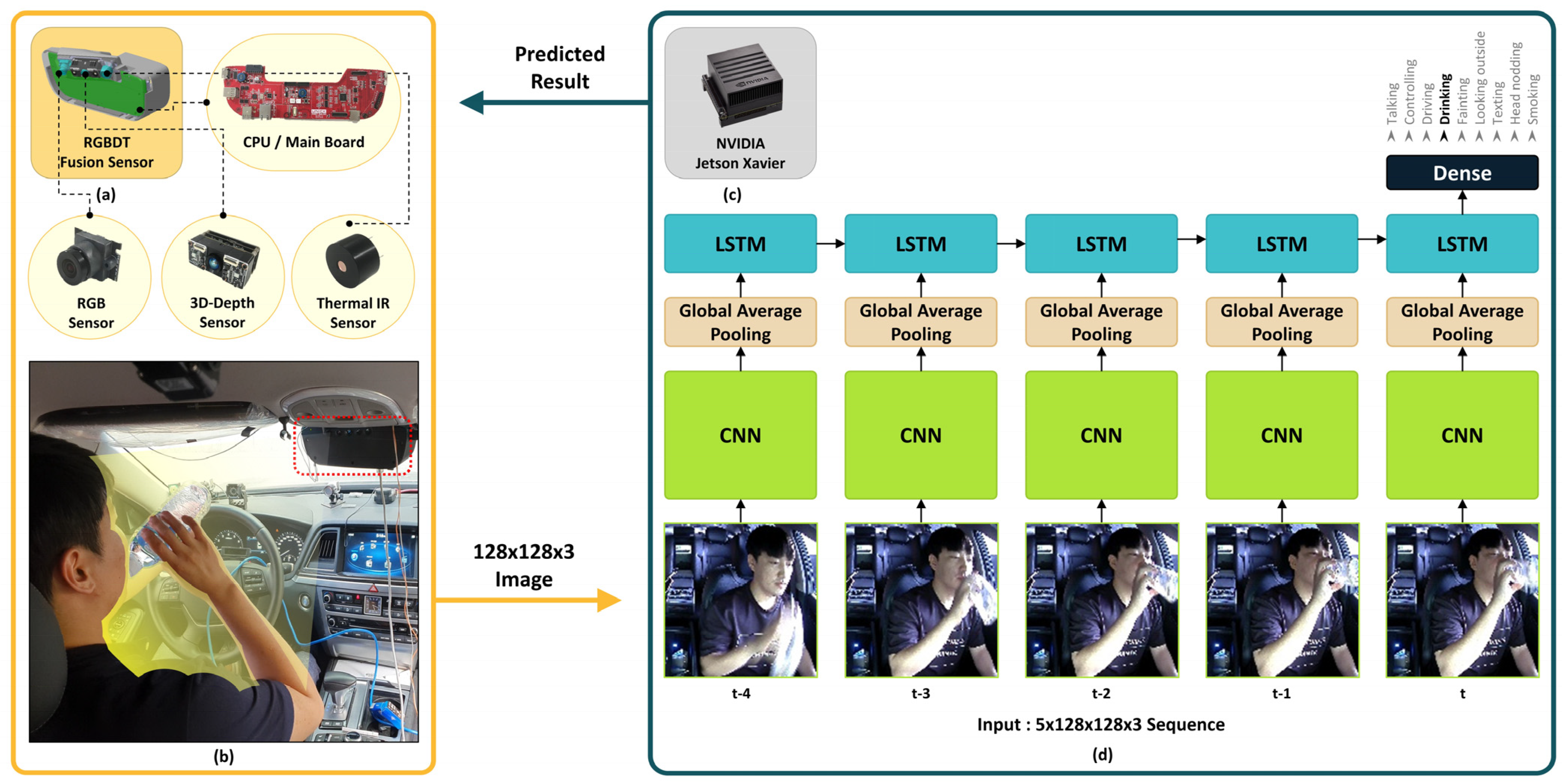
2.2. RGBDT Module Sensor

In this work, an RGBDT sensor module was applied which comprises RGB, depth, and thermal infrared sensors. Most existing driver behavior recognition approaches have mainly used RGB sensors or visible RGB images due to their wide availability. However, the lighting conditions represent one of the most challenging problems when dealing with RGB images. The RGB sensor applied in this study was capable of capturing 1280 (H) × 720 (V) pixels with a 30 fps frame rate. In addition, the thermal IR sensor captures the driver activity with 1–200 Hz (Full) and 4–800 Hz (Quarter) frame rates which can also view up to 120 × 90° within a temperature range of 20 to 85 °C. The 3D depth sensor can capture 640 × 480 pixels with a frame rate of 10 fps at a range of 0.2 m up to 2.5 m. However, in this work, only RGB and IR sensors were considered.

3. Methodology

This section describes the implementation strategy of the proposed model along with the data preprocessing methods. Moreover, the framework of the unified LRCN architecture and the training scheme are demonstrated.

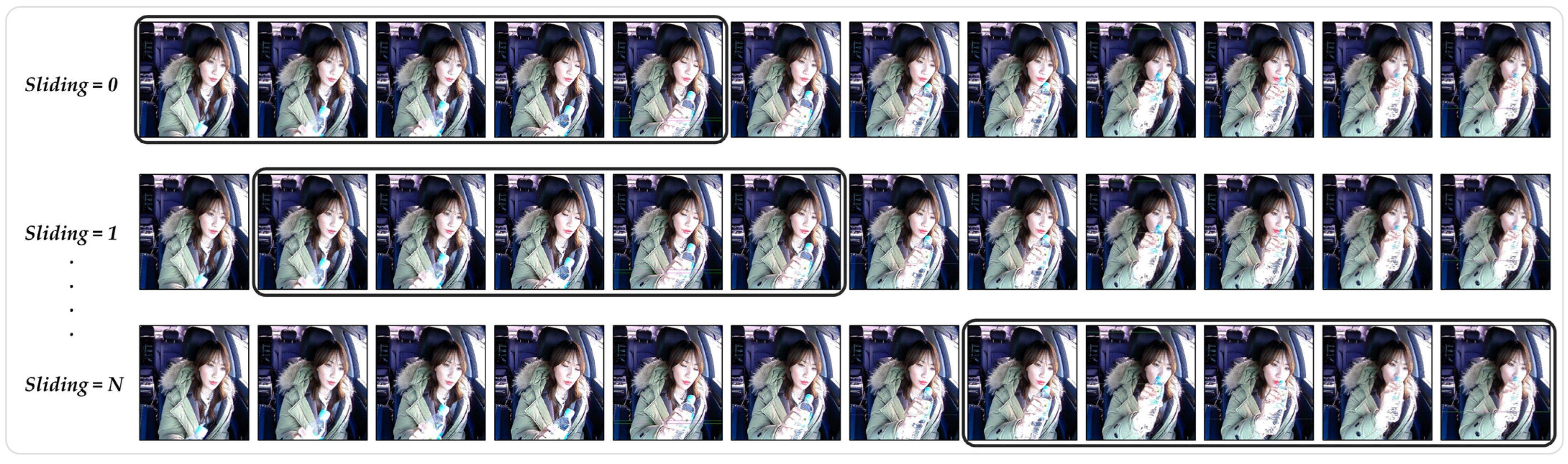
3.1. Input Data Pre-Processing

The pre-processing system comprises three minor steps including cropping, resizing, and normalizing. Recall that the original images were first stored with resolutions of 1280 × 720 and 640 × 480 for the RGB and IR images, respectively. Therefore, the raw images are first cropped to view the driver’s side only. At this stage, the cropped image size becomes 640 × 720 for the RGB images and 320 × 480 for the IR images. Employing such high-resolution images inevitably consumes high storage and computational resources. Therefore, the images are further downsized to 128 × 128 in terms of width and height without losing the essential driver body features to classify the driver activity. Note that the proposed input size image has a lower input size than that of the original pre-trained VGG16 [32] architecture, which is preferable in saving the computational source.

Then, the datasets are structured and prepared for implementing a sliding window transformation throughout the whole dataset. Figure 5 illustrates the process of the sliding window. It is similar to the sliding window across a prior observation in which the window width is fixed to five time steps. We also consider three-, four-, and six-time step inputs. However, the overall accuracy of the model witnessed a decrease when the number of frames was set to three, four, and six. The details of the number of frames’ comparative results are presented in Appendix A,

Table A1. Number of trainable parameters and feature memory of the proposed model.

Layer	Output Shape	Trainable Parameter	Feature Memory
Input layer	$5\times 128\times 128\times 3$	0	0.24 M
Conv2D 1	$5\times 128\times 128\times 64$	1792	5 M
Conv2D 2	$5\times 128\times 128\times 64$	36,928	5 M
MaxPooling2D	$5\times 64\times 64\times 64$	0	1 M
Conv2D 2	$5\times 64\times 64\times 128$	73,856	2.5 M
Conv2D 2	$5\times 64\times 64\times 128$	147,584	2.5 M
MaxPooling2D	$5\times 32\times 32\times 128$	0	0.5 M
Conv2D 3	$5\times 32\times 32\times 256$	295,168	1 M
Conv2D 3	$5\times 32\times 32\times 256$	590,080	1 M
Conv2D 3	$5\times 32\times 32\times 256$	590,080	1 M
MaxPooling2D	$5\times 16\times 16\times 256$	0	0.32 M
Conv2D 4	$5\times 16\times 16\times 512$	118,016	0.65 M
Conv2D 4	$5\times 16\times 16\times 512$	2,359,808	0.65 M
Conv2D 5	$5\times 16\times 16\times 512$	2,359,808	0.65 M
MaxPooling2D	$5\times 8\times 8\times 512$	0	0.8 K
Conv2D 5	$5\times 8\times 8\times 512$	2,359,808	0.1 M
Conv2D 5	$5\times 8\times 8\times 512$	2,359,808	0.1 M
Conv2D 5	$5\times 8\times 8\times 512$	2,359,808	0.1 M
MaxPooling2D	$5\times 4\times 4\times 512$	0	40 K
TimeDis	$5\times 512$	14,714,688	12.5 K
LSTM	256	787,456	0.2 K
Dense	1024	263,168	1 K
BN	1024	4096	1 K
Dropout	1024	0	1 K
Dense	512	524,800	0.5 K
BN	512	2048	0.5 K
Dropout	512	0	0.5 K
Dense	9	4617	-
Total	-	16 M	90 M

Conv2D, TimeDis, and BN stand for the convolutional 2D neural network, time distributed layer, and batch normalization, respectively. 16 M corresponds to the 16 million trainable parameters, while 90 M refers to the 90 megabytes (total feature memory $\times$ 4 bytes) of memory usage.

. Initially, the window discovers the first five images and uses them as input to the classifier network. Then, as shown in Figure 5, the window slides to the right side by one and applies the next five series image as the second input. This process is repeated until the window covers the entire dataset.

3.2. Proposed Model Framework

Our proposed method synergistically combines TimeDis-CNN and LSTM deep learning tools designed to receive a sequence of input data and static output with a number of frames extracted from a video as input to predict a single label of the driver behavior class. As shown in Figure 1, the proposed system takes a series of five consecutive images as an input to the convolutional network. Then, the spatial feature information of each input image is extracted by the CNN. To facilitate faster training and combat the overfitting issue, we deployed a pre-trained CNN that can extract the spatial feature of each driver image input. Specifically, we used the VGG16 [32] architecture, as it has been shown to generalize on our datasets better than a few other experimental pre-trained models (see Section 4.1). VGG16 is a pre-trained architecture originally designed to classify 1000 categories on very large-scale ImageNet [38] datasets that contain over one million images.

The original VGG16 architecture has nearly 140 million parameters, of which the fully connected layer has the most since it consists of a large number of parameters to be trained. However, this inevitably leads to high computational costs and a long training time. Therefore, in this proposed model, the fully connected layer is excluded and the LSTM layer is concatenated to perform end-to-end fine tuning. Then, LSTM uses the extracted sequence images to further explore the temporal dynamic information related to each driver activity. Afterward, the LSTM layer transforms the abstract feature vectors outputted from the time-distributed convolutional layer into an understandable representation for the fully connected dense layer. Thereby, a fully connected dense layer gathers the LSTM outputs and learns the driver’s behavior representation. In the end, the n-class, where n denotes the labeled driver behavior class, of the softmax layer is applied, which chooses the most probable labeled class among the nine driver behavior classes. More details of the unified network working principles are introduced in the following sections.

3.3. Spatial Feature Extraction

This CNN is the most dominant source and powerful tool for feature extraction and representation of images. When the inputs are sequence data (video data), each input frame is represented by the CNN feature. Training a deep CNN for image classification requires a thousand large-scale datasets. Thus, it is common to reuse a pre-trained architecture such as VGG-16 [32], AlexNet [34], ResNet [35], or MobileNet [39] by utilizing transfer learning, to leverage the knowledge gained for one task to solve the related ones to overcome the isolated learning system. As such, this study adopts VGG-16, which was originally proposed for image classification and has proven its effectiveness in feature extraction.

Figure 6 illustrates the schematic diagram of the proposed unified LRCN network. Originally, the VGG16 was composed of 13 convolutional layers, 4 pooling layers, and 3 fully connected layers, and the input size was 224 × 224 × 3, which represents the width × height × channels, respectively. Note that the fully connected layer of this architecture is removed in this work. This allows us to vary the input size image differently from the original input size. As such, our input size image was downsized to 128 × 128 × 3 with five time step inputs; this is 42% less than the original CNN architecture input size and can highly contribute to reducing the computational memory. In Figure 6, b, n, h, w, and c correspond to the batch size, time steps, height, width, and the dimension of the output feature map, respectively. Every spatial location in the output feature map corresponds to the same locations in the input feature map.

All of the thirteen convolutional layers of the CNN include 3 × 3 filters with stride one and padding one, 2 × 2 max-pooling with a stride of two, and a ReLU activation function to minimize the feature maps to half their size. Here, the pre-trained CNN network plays a key role in facilitating a robust feature extraction using both the convolutional 2D (Conv2D) and max-pooling layers. The other main reason for removing the fully connected layer is that the neuron activation occurs in the dense layer and is not capable of encoding the spatial information features, which is very essential for the next LSTM unit to capture the motion information of the sequential inputs. Unlike the Conv3D in [40] that performs the spatio-temporal operation which can be computationally intensive, the deployed Conv2D only performs the spatial feature operation to extract the primary spatial information of the driver activity image inputs and leaves the temporal extraction task to the LSTM unit. The Conv2D operation performed to extract the spatial features is expressed as follows:

$${\mathrm{C}}_{2\mathrm{D}}\left(\mathrm{a},\mathrm{b}\right)=\left(\mathrm{K}\mathrm{\ast }\mathrm{I}\right)\left(\mathrm{a},\mathrm{b}\right)=\sum _{\mathrm{x}=-\mathrm{k}}^{\mathrm{k}}\sum _{\mathrm{x}=-\mathrm{k}}^{\mathrm{k}}\mathrm{K}\left(\mathrm{x},\mathrm{y}\right)\mathrm{I}\left(\mathrm{a}-\mathrm{x},\mathrm{b}-\mathrm{y}\right),$$

(1)

where I, K, and * indicate the two-dimensional input image, 2D kernel, and convolutional operation, respectively. $\left(\mathrm{a},\mathrm{b}\right)$ is the element of the 2D input image tensor I, and ($\mathrm{x},\mathrm{y}$) is the index of the kernel filter. To achieve the Conv2D operation for all time-step inputs, the time distributed layer is applied as described in Section 3.5.

3.4. Long Short-Term Memory Network for Sequence Inputs

This LSTM [41] is a recurrent module designed for sequence processing. Generally, CNNs are capable of extracting only the local spatial information of images. However, they fail to capture the long-distance dependency of temporal learning. Thus, we apply an LSTM network, which addresses this limitation by sequentially modeling each image across multiple input data. The major contribution of LSTM is its memory cell, which accumulates state information over a long duration. As shown in Figure 7, a standard LSTM unit comprises an input gate, output gate, and forget gate. All of the gate units have a sigmoid non-linearity which squashes the real value input into a range of [0, 1], while the input units can have any squashing non-linearity. The gate’s equation can be computed using the following set of equations. The ${\mathrm{i}}_{\mathrm{t}},{\mathrm{o}}_{\mathrm{t}}$, $\mathrm{a}\mathrm{n}\mathrm{d} \mathrm{f}\mathrm{t} \mathrm{r}\mathrm{e}\mathrm{p}\mathrm{r}\mathrm{e}\mathrm{s}\mathrm{e}\mathrm{n}\mathrm{t}$ the input gate, output gate, and forget gate, respectively.

$${\mathrm{i}}_{\mathrm{t}}=\mathsf{\sigma }\left({\mathrm{W}}_{\mathrm{x}\mathrm{i}}{\mathrm{X}}_{\mathrm{t}}+{\mathrm{W}}_{\mathrm{h}\mathrm{i}}{\mathrm{h}}_{\mathrm{t}-1}+{\mathrm{b}}_{\mathrm{i}}\right),$$

(2)

$${\mathrm{f}}_{\mathrm{t}}=\mathsf{\sigma }\left({\mathrm{W}}_{\mathrm{x}\mathrm{f}}{\mathrm{X}}_{\mathrm{t}}+{\mathrm{W}}_{\mathrm{h}\mathrm{f}}{\mathrm{h}}_{\mathrm{t}-1}+{\mathrm{b}}_{\mathrm{f}}\right),$$

(3)

$${\mathrm{o}}_{\mathrm{t}}=\mathsf{\sigma }\left({\mathrm{W}}_{\mathrm{x}\mathrm{o}}{\mathrm{X}}_{\mathrm{t}}+{\mathrm{W}}_{\mathrm{h}\mathrm{o}}{\mathrm{h}}_{\mathrm{t}-1}+{\mathrm{b}}_{\mathrm{o}}\right),$$

(4)

$${\mathrm{c}}_{\mathrm{t}}={\mathrm{f}}_{\mathrm{t}}\circ {\mathrm{c}}_{\mathrm{t}-1}+{\mathrm{i}}_{\mathrm{t}}\circ \tanh \left({\mathrm{W}}_{\mathrm{x}\mathrm{i}}{\mathrm{X}}_{\mathrm{t}}+{\mathrm{W}}_{\mathrm{h}\mathrm{i}}{\mathrm{h}}_{\mathrm{t}-1}+{\mathrm{b}}_{\mathrm{i}}\right),$$

(5)

$${\mathrm{h}}_{\mathrm{t}}={\mathrm{o}}_{\mathrm{t}}\circ \tanh \left({\mathrm{c}}_{\mathrm{t}}\right),$$

(6)

where ${\mathrm{c}}_{\mathrm{t}}$, ${\mathrm{h}}_{\mathrm{t}}$, and σ stand for the memory cell, hidden state, and sigmoid function, respectively. For a particular time step t, the forget gate decides which information to clear or keep from the memory state cell by observing the new input sequence x = ${\mathrm{x}}_1,{\mathrm{x}}_2,\dots ,{\mathrm{x}}_{\mathrm{t}}$. Here, at time step t, the feature x_t is extracted from the pretrained VGG16 architecture and passed to the LSTM unit. Then, the input gate determines how the extent of information from the input will alter the data contained in the cell state. Lastly, the output gate is in charge of determining what output from the internal cell state is used as the output h_t. Then, the hidden unit state is calculated by tanh activation and the memory cell. W, b, and $\circ$ denote the weight matrix, bias vector, and element-wise product, respectively. Our proposed LSTM layer is constructed with 256 memory cells to process each frame of the sequence and store only the crucial features of each input image while learning.

3.5. The Designed LRCN Model

Our unified LRCN model receives a sequential ${\mathrm{x}}_1,{\mathrm{x}}_2,\dots ,{\mathrm{x}}_{\mathrm{t}}$ and outputs a scalar $y$ with the purpose of many-to-one prediction. Commonly, CNN receives one image or can have a fixed single input when using a pre-trained CNN architecture like VGG16 in this work. In the case of several image inputs (five sequences of inputs in this work), we apply the CNN architecture to each input image without merging the multiple images into one, and pass the output to the LSTM as a single time step. We employ a Keras TimeDistributed (TimeDis) layer to wrap the entire CNN input model to process a sequential frame as a sequence input. This TimeDis layer applies the same layer to every temporal slice input, which is essential to deal with time-series data or video frames.

In other words, instead of applying several input architectures, only one model can be applied to process each input. As such, the input shape with a time-distributed layer becomes time step, width, height, and channel. At this moment, the TimeDis layer allows the same Conv2D operation as described in Equation (1), independently to every temporal slice input (time steps), and the same set of weights is used at each timestamp. Here, the feature comes to the sequential learning stage, and the temporal information across the image frames can be learned and stored in the LSTM unit. Then, the deployed 256 hidden units of the LSTM encoder take the vector of the input sequence attributes and transform them, typically through a sigmoid activation in the hidden unit layers into a new feature vector. The total trainable parameter of the proposed LRCN network was around 16 million; this is 87% less than the original VGG16 CNN architecture.

To accelerate the convergence of the unified LRCN model, we applied a ReLU activation in each convolutional layer and on the few dense layers, as shown in Figure 6. This layer adds nonlinearity to the network and produces non-saturating gradients for the non-negative net inputs. The activation function value ${\mathrm{a}}_{\mathrm{i},\mathrm{j},\mathrm{k}}$ can be computed as

$${\mathrm{a}}_{\mathrm{i},\mathrm{j},\mathrm{k}}=\mathrm{m}\mathrm{a}\mathrm{x}\left(0,{\mathrm{x}}_{\mathrm{i},\mathrm{j},\mathrm{k}}\right).$$

(7)

The $\mathrm{m}\mathrm{a}\mathrm{x}$ ($·$) operation of the ReLu activation enables it to compute much more quickly than the other activation functions, where ${\mathrm{x}}_{\mathrm{i},\mathrm{j},\mathrm{k}}$ is the activation value and the input of the activation function at the location of ($\mathrm{i},\mathrm{j}$) on the ${\mathrm{k}}^{\mathrm{t}\mathrm{h}}$ channel [42].

In the proposed network, several connections that learn the non-linear relation are usually co-adapted, which causes overfitting issues. As such, to combat the overfitting problem, an aggressive dropout of 0.9 is applied in the dense layer of the unified network. This aggressive dropout introduces an excessive random dropping of some connections or units and ultimately enhances the generalization ability of the proposed network. The dropout output $y$ is computed using an element-wise multiplication of the binary vector of the size m drawn from a Bernoulli distribution r and the activation function layer $\mathrm{a}$ as shown in the Equation (8):

$$\mathrm{y}=\mathrm{r}\circ \mathrm{a}\left({\mathrm{W}}^{\mathrm{T}}\mathrm{x}\right),$$

(8)

where $\mathrm{W}\in {\mathbb{R}}^{\mathrm{n}\times \mathrm{m}},$ and $\mathrm{x}=[{\mathrm{x}}_1,{\mathrm{x}}_2,\dots ,{\mathrm{x}}_{\mathrm{n}}]$ is the weight matrix and the input vector to the dense layer, respectively [43].

In addition, since the CNN layer has a lower trainable parameter, it is unlikely to contribute as strongly as a fully connected layer to the overfitting issue. As such, no batch normalization (BN) is used in the CNN layer; it is only applied in the dense layer to regularize the model, and thus reduce the repetitive usage of the dropout layer. Moreover, this BN layer minimizes the inner covariate shift problem by normalizing the variance and means of the layer inputs, where the approximation of the variance and mean are computed after every mini-batch instead of the whole training set. Assuming the input layer $\left[{\mathrm{x}}_{\mathrm{n}}={\mathrm{x}}^1..{\mathrm{x}}^{\mathrm{k}}\right]$ with k dimensional input, typically, we normalize the n^th dimension as follows:

$$\mathrm{B}\mathrm{N}\left({\mathrm{X}}_{\mathrm{n}\mathrm{o}\mathrm{r}\mathrm{m}\mathrm{a}\mathrm{l}\mathrm{i}\mathrm{z}\mathrm{e}}\right)={\displaystyle \frac{{\mathrm{x}}_{\mathrm{n}}-{\mathsf{\mu }}_{\mathrm{m}}}{\sqrt{{\mathsf{\sigma }}_{\mathrm{m}\mathrm{b}}^2+\mathrm{c}}}},$$

(9)

where ${\mathsf{\mu }}_{\mathrm{m}}$, ${\mathsf{\sigma }}_{\mathrm{m}\mathrm{b}}^2$, and $\mathrm{c}$ are the mean, variance, and constant value of the mini-batch, respectively [44]. The final step in predicting the driver class is carried out by the softmax layer; as defined in the equation below, the softmax $\mathrm{S}\left({\mathrm{y}}_{\mathrm{i}}\right)$ gives the probability distribution over the nine predetermined driver behavior classes.

$$\mathrm{S}\left({\mathrm{y}}_{\mathrm{i}}\right)={\displaystyle \frac{{\mathrm{e}}^{{\mathrm{y}}_{\mathrm{i}}}}{\sum _{\mathrm{j}=1}^{\mathrm{D}}{\mathrm{e}}^{{\mathrm{y}}_{\mathrm{j}}}}},$$

(10)

where $\mathrm{D}$ corresponds to the probability of the data belonging to one of the nine driver activity classes, and ${\mathrm{e}}^{{\mathrm{y}}_{\mathrm{i}}}$ and ${\mathrm{e}}^{{\mathrm{y}}_{\mathrm{j}}}$ represent the standard function of the input vector and output vector, respectively.

3.6. Model Training

The experiments for RGB and IR images were first performed separately with the same networks. This gave us a baseline to compare the results of the two different image sources. The classifier network inputs are set to five time steps and fed to the unified LRCN architecture. To perform end-to-end fine tuning, the pre-trained CNN architecture is kept trainable throughout the whole experiment. When training a deep learning model, the network hyperparameters such as the optimizer, learning rate, the number of hidden units in LSTM, and the dense layer can greatly affect the tradeoff accuracy. Particularly, the number of dense layers and learning rate exert large effects on the complexity of the designed model, as well as the accuracy.

As such, the hyperparameters are carefully analyzed and selected in this work. Regarding the LSTM hidden units, we compared 256 units and 512 hidden units and found that the model with 256 hidden units yielded superior results. Therefore, the number of hidden units for the LSTM layer in this proposed work was set to 256. The dense layer was set to single 1,024 nodes and 512 nodes, each followed by batch normalization and dropout of 0.5 and 0.9, respectively. An aggressive dropout (0.9) was applied to combat the overfitting problem. The batch size and number of epochs were selected to be 24 and 300, respectively. To optimize the weights of the proposed network, the Adam optimizer with a learning rate of 1 × 10⁻⁶ was set as an objective function. In addition, the model recognition performance was measured using categorical cross-entropy loss, whose result output was a probability value between 0 and 8. The standards loss function ${\mathrm{C}}_{\mathrm{l}\mathrm{o}\mathrm{s}\mathrm{s}}$ was computed using the number of driver activity label classes l, the target label class ${\mathrm{m}}_{\mathrm{i}}$ and the logarithm of the ${\mathrm{i}}^{\mathrm{t}\mathrm{h}}$ value in the final model output ${\stackrel{⏜}{\mathrm{m}}}_{\mathrm{i}}$ as shown in Equation (11).

$${\mathrm{C}}_{\mathrm{l}\mathrm{o}\mathrm{s}\mathrm{s}}=-\sum _{\mathrm{x}=1}^{\mathrm{l}}{\mathrm{m}}_{\mathrm{i}}·\mathrm{l}\mathrm{o}\mathrm{g}{\stackrel{⏜}{\mathrm{m}}}_{\mathrm{i}}.$$

(11)

To learn robust features from the unified LRCN model, overcome the imbalanced data between the 9 classes, and increase the diversity of our training set, we applied various data augmentation strategies. This also helped to reduce the dependence of the proposed model on spurious characteristics and increase the generalization ability. As such, rotation either clockwise or counterclockwise, zooming in, and zooming out augmentation techniques were applied to regulate the changes in the pose of the camera sensor and to cope with changes in the size of the driver due to fluctuations of the driver’s seat position which can occur while driving. A gamma correction was also utilized with a gamma value of 1.0 to manipulate the brightness and intensity of the sequence image caused by sunlight and illumination. The remaining data augmentation techniques were saturation changing and adding salt and pepper noise. Note that the input data of our model is not a single image but a sequence of five series images. Thus, the augmentation strategy has to be performed sequence by sequence instead of image by image. In this sense, a randomly selected augmentation method is applied for every sequence input.

The adjustable parameters used in each augmentation method were selected randomly within the predetermined range. For instance, when applying a rotation to the five sequence inputs, the parameter is the angle at which the image randomly rotates between the range of [−10, +10] degrees. At this moment, all five input images rotate at an equal angle without losing the original information. To implement the augmentation system, Keras provides a data generator application programming interface (API), where we can load all of the image data and perform the augmentation process for a single type of input image. However, our model has a sequence type of input and contains a huge amount of data, such that it would be impossible to load all of the data at once for training. Thus, we built a custom data generator that enables us to load a part of the dataset by batch size and perform the augmentation system, which is then fed to the model dynamically. Notice that the augmentation strategy is inactive, or no data augmentation technique is applied to the testing set. Therefore, only the sequence inputs will be augmented.

3.7. Experiment Environment

All of the experiments were conducted using the Python three programming environment on a personal computer equipped with an NVIDIA GeForce GTX TITAN GPU running Ubuntu18.06. The network was then trained using the TensorFlow 2.2 and Keras 2.3.1 frameworks.

4. Results and Evaluation

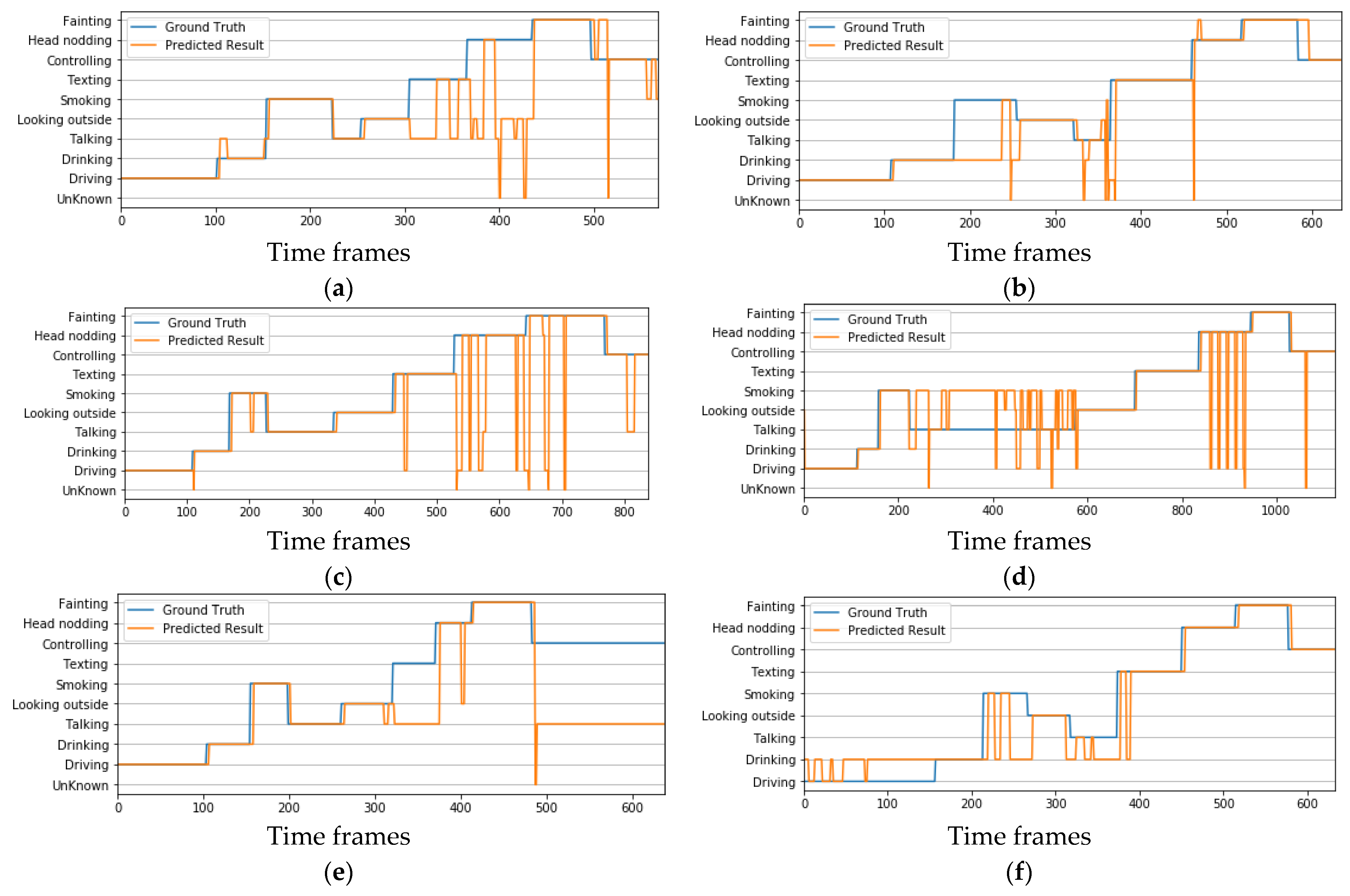
4.1. Evaluation of the LRCN Model Based on Train–Test Split

For fair performance evaluation of the unified LRCN and single CNN architecture, we performed a comprehensive experiment based on the data collected in the second phase that contains 17 participants for RGB and IR images. A train–test split method was implemented in which fifteen drivers were set as training and the remaining two as testing. At this time, single image input was considered for all VGG16, ResNet50, MobileNet, Xception, DenseNet169, NASNet-Mobile, and InceptionResNetV2 pre-trained CNN architectures. In contrast, a stack of five sequence inputs was used for the unified LRCN model including VGG16+LSTM, ResNet50+LSTM, MobileNet+LSTM and Xception+LSTM. To demonstrate the superiority of the models, the experiment was conducted under the same hyperparameters for both architectures.

As such, a stochastic gradient was applied to update the parameters with a learning rate of 0.001. The batch size and the number of epochs were set to 24 and 60, respectively. The dense layer has two 1024 nodes, each followed by a dropout probability of 0.5, and one final 512 node dense layer was added to interpret the summary of the input sequence. Note that this section of the experiment was carried out for two main reasons. First, the effect of the LSTM model was evaluated based on the sequence inputs. Particularly, the superiority of the models between a single input image of the CNN architecture and a sequential input of the CNN-LSTM model was evaluated.

Second, an effective pre-trained CNN feature extractor that generalizes well for our datasets among the experimented pre-trained models was selected. For this reason, the same hyperparameters were set for all architectures, as described above. As

Table 1. This performance evaluation between CNN and TimeDis CNN+LSTM based on the train–test split.

Model	Test Accuracy (%)
TimeDis VGG16+LSTM	86.53
VGG16	77.08
TimeDis ResNet50+LSTM	77.46
ResNet50	65.83
TimeDis MobileNet+LSTM	78.84
MobileNet	68.57
TimeDis Xception+LSTM	73.29
Xception	70.12
DenseNet169	74.65
NASNet-Mobile	66.92
InceptionResNetV2	66.68

The CNN+LSTM corresponds to the CNN concatenated to the LSTM unit through the TimeDistributed (TimeDis) layer. For all the CNN architecture and CNN+LSTM models, the same hyperparameters were set for fair comparison purposes.

reveals, the overall performance of the pre-trained CNN with LSTM is superior to all other single pre-trained CNNs. Specifically, the accuracy comparison depicted VGG 16 combined with LSTM as the most accurate. Although ResNet showed higher classification accuracy in the 2015 ILSVRC (ImageNet Large Scale Visual Recognition Challenge) competition among pre-trained models, it is a very deep architecture compared to VGG16 and the other most pretrained models. As a result, it requires relatively large-scale datasets to perform well. Based on this experiment, the VGG16 combined with LSTM was chosen as the proposed model and further modified, including the hyperparameters, to improve its classification accuracy for all driver participants.

4.2. Evaluation of the LRCN Model Based on Seven-Fold Cross Validation

In this subsection, the driver activity for all 31 drivers was evaluated based on k-fold (k ranges from one to seven) cross-validation to check the generalization ability of the model on new datasets. Therefore, the dataset is divided into seven subsets or folds base on the number of drivers. As such, each time, one of the seven subsets was used as a testing set, and the rest were put together to form a training set. Note that the training and testing sets in each iteration never originated from the same driver. Thus, the model receives completely unseen data as a testing set. In this way, the model can be evaluated effectively to determine the predictive ability on various unseen datasets. In each fold, both RGB and IR images are considered in the training as well as the testing set, so that the model can learn to recognize the driver’s activity without limitations of time for both day- and nighttime conditions. From the results acquired in the above section of the experiment, we observed that the model hyperparameters exhibited symptoms of high variance, which confirms the overfitting of the unified LRCN model. Therefore, the hyperparameters were carefully analyzed and modified, and finally set as proposed parameters (see Section 3.6).

Table 2. The performance metric measures (Accuracy, Precision, Recall, and F1 score) based on seven-fold cross validation for RGB images.

Metrics	Fold-1	Fold-2	Fold-3	Fold-4	Fold-5	Fold-6	Fold-7	Average
Accuracy (%)	90.1	85.60	88.6	78.7	94.6	92.9	90.6	88.7
Precision (%)	86.7	82.7	85.9	83.7	95.6	89.4	91.6	87.9
Recall (%)	82.3	81.9	87.7	87.2	93.8	88.3	88.1	87.0
F1-Score (%)	83.5	80.1	86.2	82.8	94.6	88.6	89.4	86.5

and

Table 3. The performance metric measures (Accuracy, Precision, Recall, and F1 score) based on seven-fold cross validation for IR images.

Metrics	Fold-1	Fold-2	Fold-3	Fold-4	Fold-5	Fold-6	Fold-7	Average
Accuracy (%)	94.9	82.9	96.7	95.3	96.4	86.9	93.8	92.4
Precision (%)	92.9	78.2	95.9	93.7	97.2	86.4	95.3	91.4
Recall (%)	92.6	75.2	96.3	92.7	95.9	85.0	93.4	90.2
F1-Score (%)	92.3	74.9	96.4	92.2	96.3	84.6	94.0	90.1

illustrate the classification results assessed using cross-validation for each fold and the overall performances of the models for RGB and IR images, respectively. The performance of the model was determined by averaging the seven-fold cross-validation. Fold-1 to Fold-7 represent the seven-fold cross validation. For multi-class classification, alongside accuracy, it is good practice to evaluate the model with additional evaluation metrics to further assess the model’s robustness. Therefore, an additional three standard performance indicators, namely, precision, recall, and F₁-score, were computed for each fold and used to determine the average output. The precision is the ratio of the true positives to the total of the true positives and false positives (when the model predicts non-distracted driving while it is actually getting distracted). The recall is the ratio of the true positive to the summation of the true positives and false negatives (when the classifier does not detect non-distracted driving). In this sense, recall and precision are complementary and this characterization manifests useful information when they are mingled using the F_1-score, which shows the harmonic mean of the precision and recall.

According to the results shown in Table 2 and Table 3, it can be seen that there is a clear accuracy difference in each fold. This is mainly because the model in each iteration receives various unseen data. In particular, the highest fold accuracy of the model for RGB and IR images was 94.6% and 96.7%, respectively. In contrast, the lowest accuracy is observed in fold four and fold two for RGB and IR images, respectively. In

Table 4. Average Precision, Recall and F₁ score of the nine class categories for RGB images and IR images.

	RGB Images			IR Images
Driver State	Precision (%)	Recall (%)	F1-Score (%)	Precision (%)	Recall (%)	F1-Score (%)
Talking	78.4	78.7	76.1	90.1	95.1	92.4
Controlling	85.0	87.3	83.6	95.4	96.7	95.6
Driving	95.0	87.0	89.4	98.0	98.9	98.6
Drinking	92.4	92.1	92.3	93.9	94.6	93.7
Fainting	86.4	84.4	84.3	89.1	84.9	86.0
Looking outside	86.9	88.7	87.4	94.6	99.1	96.6
Texting	93.1	96.3	94.7	98.3	93.0	95.3
Head nodding	84.7	81.1	81.7	82.7	75.0	77.4
Smoking	89.4	88.1	88.6	81.3	74.1	75.7

, the recognition result for each label is reported. For RGB images, texting resulted in the highest F₁ score.

A similar performance was observed in the drinking class. This could be due to driver activities involving objects such as phones and plastic bottles being easier to detect by the classifier model. In contrast, the talking class showed the worst performance. We found that the talking class is mainly misclassified as smoking. Indeed, based on our class definition, talking and smoking have similar right arm movements and orientation, which leads the classifier model to a wrong prediction. As shown in Table 4 for the IR image results, except for the heading nodding and smoking class, the remaining seven classes achieved accuracies over 85%, as measured by the F1 score. The worst performance appears in the smoking class.

To further understand the performance of the classifier model, Figure 8 illustrates the final average confusion matrix of the classifier model for both RGB and IR images. First, a confusion matrix for each fold was obtained. Then, the mean average for all folds was computed. The diagonal of the confusion matrix from left to right shows the maximum result class in their perspective row and column. In general, we observed comparatively low performance in faint and head nodding classes. This result is expected, not only due to the fact that the amount of data collected for faint and head nodding classes was relatively small compared to other classes, but also because the similarity between both actions caused the classifier model to be confused. As such, we performed additional experiments by merging both actions as a single class to explore the combined result. In this case, we observed a significant accuracy rise for both types of images.

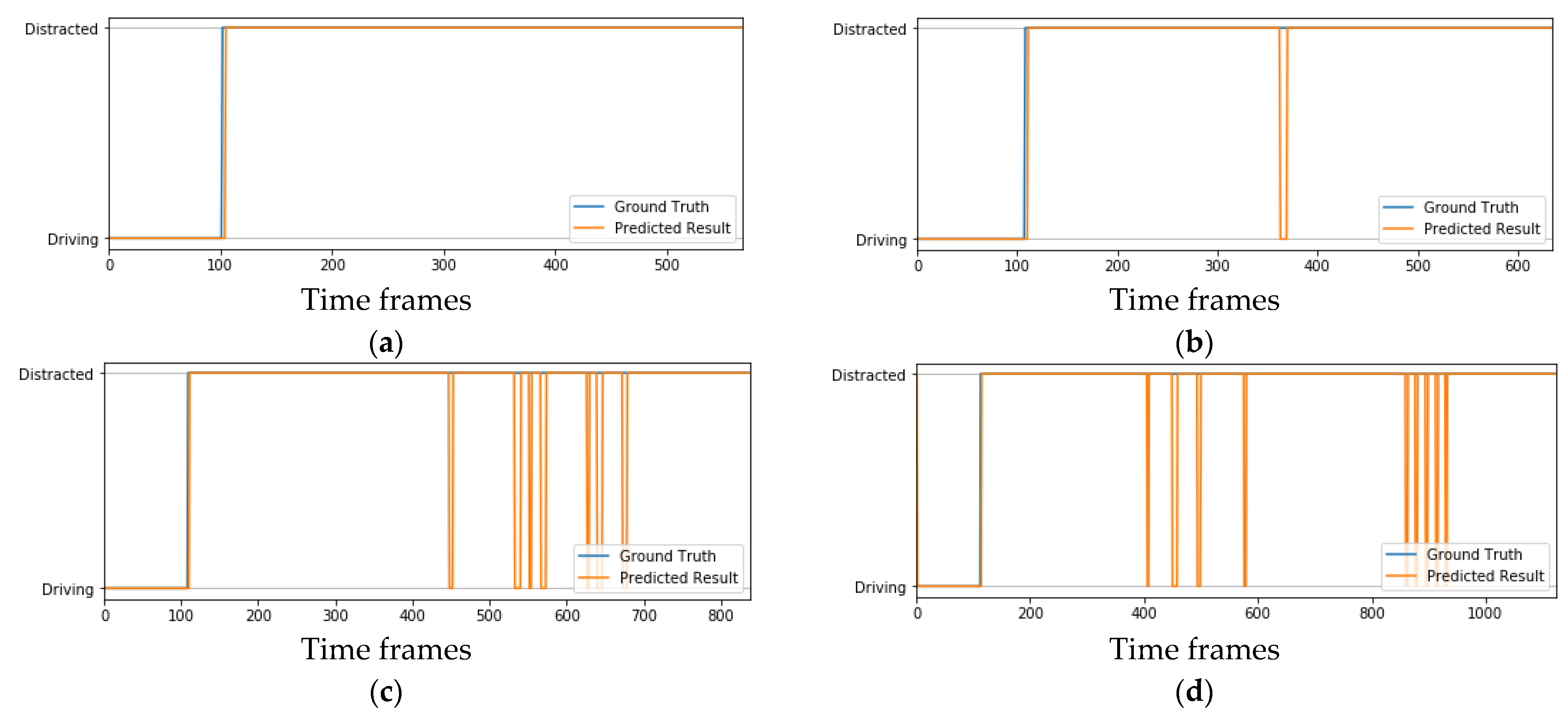
4.3. Binary Driver Distraction Classification

An alternative way to study driver behavior is to detect whether the driver is in non-distracted driving or distracted conditions. This section addresses the driver behavior with two separate binary classification tasks which detect non-distracted driving or distracted driving. In this case, all of the driver behavior classes except the driving class are combined to form a distracted driving class, whereas normal driving is considered as non-distracted driving. Likewise, for multiclass recognition, seven-fold cross-validation was computed to evaluate the performance of the binary classifier.

Table 5. Performance evaluation of the proposed model for binary classification (non-distracted driving and distracted driving) based on seven-fold cross validation.

Image Type		Fold-1	Fold-2	Fold-3	Fold-4	Fold-5	Fold-6	Fold-7	Average
RGB Images	Driving	98.9	85.8	88.7	45.0	99.0	97.9	92.6	86.8
	Distracted	96.2	96.5	98.4	99.8	97.1	98.3	96.5	97.7
	Average	97.4	91.1	95.5	83.3	97.5	98.1	95.1	93.9
IR Images	Driving	96.1	98.4	100.0	98.5	99.2	100.0	100.0	98.9
	Distracted	99.6	98.8	99.8	99.7	99.2	99.9	100.0	99.6
	Average	99.1	98.7	99.9	99.5	99.3	99.9	100.0	99.2

reports the performance of the binary classifier across the seven folds and, based on the average result, the classification accuracies were 93.9% and 99.2% for RGB and IR images, respectively.

It is worth noting that the overall performance of the model significantly increased for binary classification. For IR images, similar performance was observed for both non-distracted driving and distracted driving classes. In RGB images, the average accuracy for distracted driving appears to be superior, with a value of 97.7% along with a value of 86.8% for non-distracted driving. The reason could be that the combined distraction class data resulted in superior performance in comparison to non-distracted driving. In fact, in real-life driving scenarios, obtaining a higher detection accuracy for a distracted driving class is more necessary than for non-distracted driving, since the main intent is to identify the distracted driver and provide a warning system to reduce the potential accident risk.

4.4. Real-Time Implementation

In this section, the real-time assessment is reported. After thoroughly evaluating the developed model, the model was tested on an actual real vehicle environment to determine the capability of prediction during the day- and nighttime conditions. At this moment, four new people (three male and one female) were recruited and verbally instructed to perform the predefined actions. Normally, the vehicle environment is subjected to various limitations such as size and power. As a result, instead of using size-constrained GPU boards, we deployed an embedded NVIDIA Jetson AGX Xavier board. This device consumes less power and is much cheaper than other GPU boards. The embedded board is equipped with a 512-core GPU with tensor cores, 8-core ARM 64-bit CPU, and 32GB 256-bit LPDDR4x memory. Ubuntu 18.06 and Tensor flow were used for the OS and deep learning frameworks, respectively.

The completed trained model weight was first stored in hd5 format in our original workstation environment. Then, the hd5 weight file was converted to Tensor RT format to deploy on the embedded board. In the conversion process, a few optimizations were made to fit the operation on the embedded board. During the real-time streaming, the RGBDT sensor module and Xavier embedded board are interconnected using transmission control protocol/internet protocol (TCP/IP) communication to exchange data. At this time, the embedded board receives the driver activity image from the RGBDT sensor and creates a single sequence based on the most recent five frames of images, and uses it as an input to the loaded model. The prediction result is not immediately returned to the RGBDT sensor because the model prediction could be temporarily wrong. Instead, it selects the most repeated action or actions that appear more than three times among the five frames (single sequence) and returns them as the final predicted driver action result. This also helps to reduce the misclassification that can occur during the transition scene from one type of driver class to another type of driver class. The computational time to execute a single sequence input (composed of five frames) is around 90 ms/sequence and the general inference speed of the system is around 12 fps on the Xavier embedded board.

Meanwhile, to report the statistical results, a video was recorded during the real-time streaming in day- and nighttime conditions. Similarly to the real-time evaluation setting reported previously [17], we compared the difference between the ground truth label and the predicted driver behavior class, as shown in Figure 9 and Figure 10. In Figure 9a,b, the multiclass result of driver 1 for daytime with RGB images and nighttime with IR images are reported, respectively. During these predictions, except for the minor misclassification shown in the talking and texting class, the model produced state-of-the-art results with accuracies of 98.2% and 89.7% for day- and nighttime, respectively. Figure 10a,b illustrate the binary prediction as either non-distracted driving or distracted driving of driver 1 for daytime with RGB images and nighttime with IR images, respectively. The predictions reveal that the performance was significantly improved in both cases for a binary classification task, with accuracies of 99.6% and 97.9% for day- and nighttime, respectively.

On the other hand, the proposed model achieved accuracies of 75.8%, 92.9%, and 74.8% during the daytime, while 80.8%, 88.3%, and 75.4% accuracies were achieved during the nighttime for driver 2, driver 3, and driver 4, respectively, in the real-time assessment. A more detailed result can be found in Appendix A, Figure A1 and Figure A2. On average, the proposed model performance in real-time prediction was 85.4% and 83.6% during the daytime and nighttime, respectively, for multiclass recognition. Also, the average binary classifier performance was 98.7% and 97.2% for the daytime and nighttime scenarios, respectively. Based on the overall real-time prediction results, it can be concluded that the proposed model showed promising performance for both day- and nighttime scenarios even though there are few result fluctuations based on the type of driver. This is mainly because the drivers engaged in several non-driving activities in real-life driving different from the predefined driver activities studied in this work, and thus led the proposed system to slight misclassification. Here, it is worth noting that the model has achieved a state-of-art performance for the binary classifier that identifies whether the driver is in a non-distracted driving or distracted condition. This is very important in real-time practical use, as the main objective of building driver detection models is to give a warning whenever the driver is getting distracted regardless of which distracted activity is performed. The real-time prediction recorded video for driver 1, during both daytime and nighttime, can be found in the Supplementary Materials as Videos S1 and S2.

4.5. Comparison with Existing Approaches

In this section, we benchmark our proposed model against selected existing state-of-the-art studies. Although several features have been widely used to study the effect of driver activity on road safety, for a fair comparison, we selected studies that have similar feature inputs (images) to our study to determine the driver activity state. As shown in

Table 6. Comparison of the proposed model with other existing state of the art approaches.

Approaches	Accuracy	Participants	Platform	Operation
				Daytime	Nighttime
GMM segmentation and transfer learning [17]	Recognition: 81.6% Binary classification: 91.4%	10 drivers	Real Vehicle	$✓$	$\times$
InterCNN with MobileNet [30]	Recognition: 73.9%—9class, Recognition: 81.66%—5class	50 drivers	Mockup car (Simulator)	$✓$	$\times$
VGG16 with regularization [31]	Recognition: 96.3% (Train–Test Split)	31 drivers	Real Vehicle	$✓$	$\times$
AlexNet,VGG16, GoogleNet, and ResNet [33]	Recognition: 86–92%	10 drivers	Simulator	$✓$	$\times$
AdaBoost classifier and Hidden Markov Model [45]	Recognition: 85.0%, Binary classification: 89.8%	8 drivers	Simulator	$✓$	$\times$
Modified SVM, KNN, and RUSBoost [46]	Recognition: 66.7~87.7%	20 drivers	Real Vehicle	$✓$	$\times$
Our proposed model	Recognition: 88.7% for RGB images and 92.4% for night-time datasets. Binary classification: 93.9% for RGB images and 99.2% for nighttime datasets.	35 drivers	Real Vehicle	$✓$	$✓$

, the common limitation of most existing works [17,30,31,33,45,46,47,48,49,50] is the absence of a driver activity recognition system for nighttime scenarios. These studies adopted several techniques that can enhance the accuracy of driver activity recognition, and some meet the real-time requirement. However, due to the lack of a full-time detection system throughout the day- and nighttime conditions, we believe that this may not be suitable for practical use to integrate with the modern ADAS. Meanwhile, great effort was made in [51] by collecting a large-scale dataset (Drive & Act datasets) including RGB, infrared, and depth images to facilitate future research on activity recognition during both day- and nighttime situations.

A previous study evaluated numerous drivers by recruiting around 50 participants and achieved a reasonable result [30]. However, the whole process was conducted in a mock-up car environment. Thus, the results from the simulator may appear very different for a real vehicle environment. Another study [31] introduced various regularization techniques to their network construction process and achieved higher detection accuracy. However, the evaluation setting was based on a simple train–test split method. This evaluation system does not accurately reflect the true performance of the model, as the result highly depends on which data points end up on the training set and the testing set. In the proposed model, we integrated a seven-fold cross-validation evaluation system. This evaluation strategy has many advantages over train–test evaluation techniques since it provides observation of all of the data by making use of both training and testing techniques in the main time. Moreover, each testing set is used exactly once and, in this sense, the classifier model is not trained for the same training and testing sets.

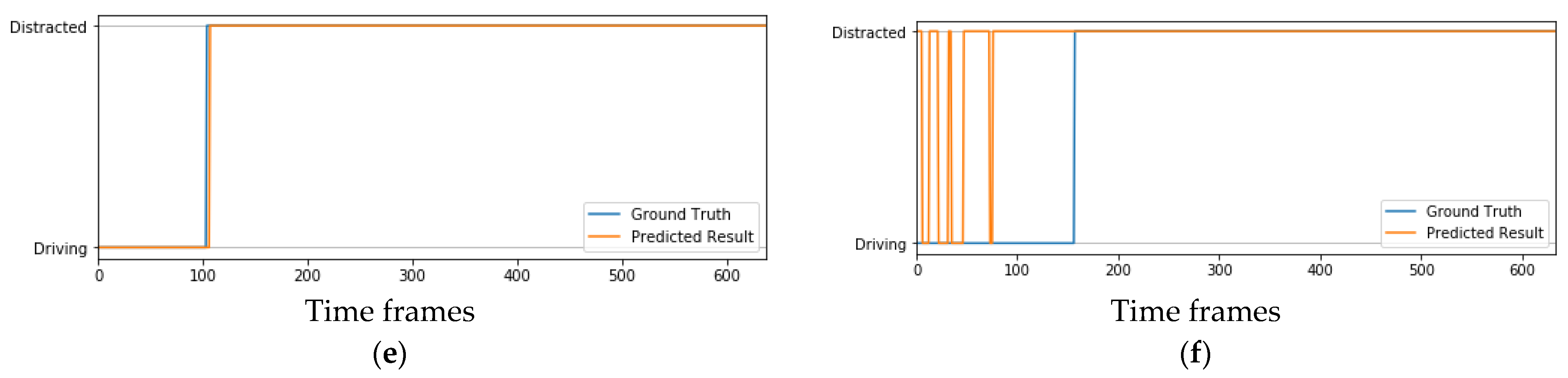
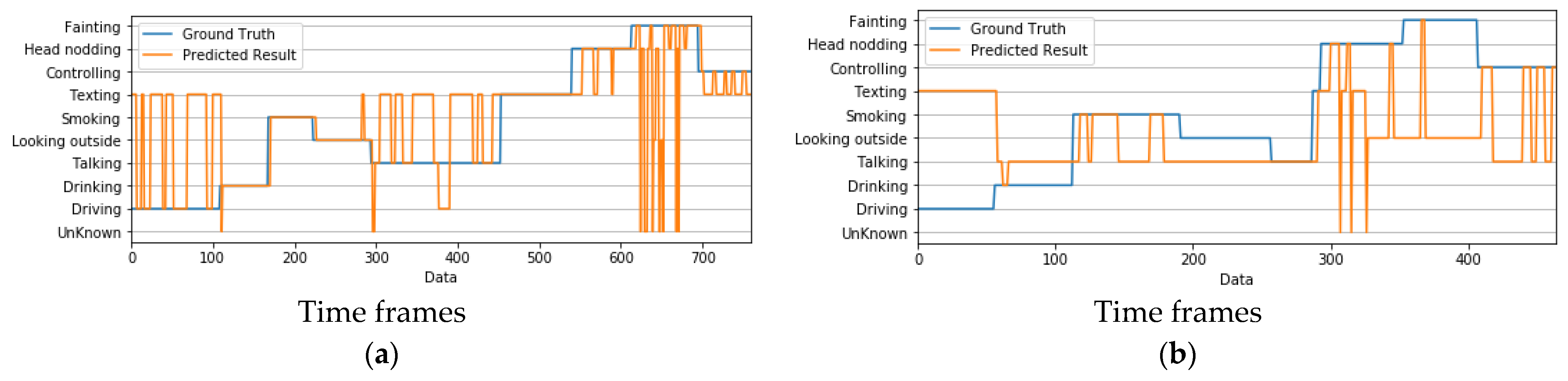
4.6. Failure Analysis of the Proposed System

This section investigates the failure analysis and limitation of the proposed LRCN model. Normally, for driver activity recognition, RGB images collected from the RGB sensor and IR images collected from the IR sensors are used for real-time applications during the day- and nighttime, respectively. However, in this work, we further studied the use of RGB images gathered at nighttime and IR images collected during the daytime. For this purpose, we collected RGB images at nighttime and IR images during the daytime for two drivers in a real-time scenario. However, the model has shown poor performance or failure for both drivers, with an accuracy of 63.69% and 30.87% for the RGB images collected at nighttime. This is because the RGB sensor is sensitive to sunlight and illumination, and therefore cannot completely capture the full posture of the driver during the nighttime. A more statistical result is presented in Appendix A, Figure A3. On the contrary, the IR images result shows a satisfactory performance, with an accuracy of 89.6% and 86.4% in the daytime. Based on the result obtained, it can be concluded that the usage of RGB sensors (RGB color images) for driver behavior recognition overnight are impractical. However, IR sensors (IR images) can be applied for both day- and nighttime driver activity recognition, as acceptable results were obtained in both scenarios.

On the other hand, despite the higher performance of our model, the system still has a few limitations in identifying the driver activities that have common body posture and orientation, such as talking and smoking, and head nodding and fainting. Specifically, talking is recognized when the driver raises their right arm to engage with a passenger, while in real-life scenarios, the driver may also engage in conversation with both hands on or off the wheel. Also, looking outside is recognized when the driver is only looking to the left outside direction; however, in real-life practice, drivers might engage in various non-driving related activities and look in various directions. Therefore, we defer this study to future work, to enrich our dataset with several driver activities and more driver samples in a complex environment and, moreover, to comprehensively confirm the robustness of IR data under various temperature conditions and with different drivers, thus maximizing the recognition and generalization ability of the proposed system to be fully deployed on a real-time basis. We also plan to incorporate the depth sensor information in the future work to evaluate its impact on the model performance.

5. Discussions and Conclusions

5.1. Discussion

This paper developed a LRCN model tailored to recognize driver activity. Generally, for driver activity, recognition backgrounds are not necessary and less informative. In particular, a complex background can negatively influence the effectiveness of driver activity recognition. Thus, learning both the spatial and temporal features by implementing a proper LSTM becomes the key way to improve driver activity recognition performance. In this sense, we aimed to emphasize the use of the LSTM model for sequence inputs and introduced a new framework for robust driver activity recognition practice without performing any traditional unwanted major preprocessing measures.

One of the limitations of developing a deep neural network is the need for large-scale datasets for training and validation. Thus, to handle this problem, we integrated transfer learning and fine tuning on a pre-trained VGG16 architecture for strong initialization of the unified LRCN model. Moreover, to improve the predictive capability of the model, the network hyperparameters were carefully analyzed and optimized. At this moment, the major challenge was that the hyperparameters are interlinked and several parameter combinations have different effects on the overall results of the model. Enhancing the parameters while optimizing the other predefined values may not result in the correct hyperparameter combination. Nevertheless, the final proposed model, which contains the optimal values of the hyperparameters, achieved superior prediction on the test datasets as well as in the real-time evaluation in comparison with the other experimented parameters.

Although the pre-trained CNN architecture applied in this study was originally trained with only RGB images while utilizing transfer learning and fine tuning with our RGB and IR images based on the designed LRCN model, in almost all cases, the IR image results showed superior performance. An in-depth understanding of the image is mainly because thermal imaging or infrared cameras work by measuring and detecting the infrared radiation emanating from objects. In other words, it only senses the difference in heat within the temperature range inside the vehicle. At this moment, the IR image provides a clear posture of the driver regardless of the cluttered background environment and sunlight. On the other hand, RGB images are easily affected by sunlight and illumination. This creates high noise when training a deep learning model and can lead to reduced performance. In addition, the ultimate aim of developing a driver activity recognition model was to integrate it with a warning system to alert drivers from being distracted, regardless of which distracted activity is performed. As a result, merging all distraction activities as one class and executing binary classification led the classifier model to tremendous state-of-the-art performance.

5.2. Conclusions

In this paper, a real-time driver activity recognition technique based on the LRCN model was proposed, which detects the driver activities in diverse day- and nighttime scenarios. Our designed model combines the TimeDistributed CNN with LSTM to utilize spatial, temporal, and spatio-temporal information. In contrast to most existing works that use a single input frame that could get confused with a sequence of frames of different driver classes, a sequential input frame was applied using both RGB and IR images to recognize the driver’s activity throughout the entire day.

Moreover, the proposed model was benchmarked against existing state-of-the-art approaches. The experiments revealed that the synergistic interplay between TimeDistributed CNN and LSTM models significantly contributes to maximizing the performance of the model. Additionally, the binary classifier, which determines whether the driver is in a non-distracted or distracted condition, achieved a promising state-of-the-art result, thereby showcasing the applicability of our approach in practical settings. With its efficient and cost-effective properties, this approach can be readily integrated into the design of ADAS to provide real-time warnings to drivers, thereby reducing potential risks. In future work, we will emphasize advancing the recognition algorithm and expanding the study to encompass a broader range of driver activities, aiming to enhance the adaptability and generalization of the model across diverse environmental conditions.

References

1. Road Traffic Injuries. Available online: https://www.who.int/news-room/fact-sheets/detail/road-traffic-injuries (accessed on 27 June 2021).
2. NHTSA Statistics. Available online: https://www.nhtsa.gov/book/countermeasures-that-work/distracted-driving/understanding-problem (accessed on 27 June 2021).
3. Lee, J.D. Dynamics of Driver Distraction: The process of engaging and disengaging. Ann. Adv. Automot. Med. 2014, 58, 24–32. [Google Scholar] [PubMed]
4. Vehicle Safety. Available online: https://www.cdc.gov/niosh/motor-vehicle/distracted-driving/index.html (accessed on 29 June 2021).
5. Ahlstrom, C.; Kircher, K.; Kircher, A. A Gaze-Based Driver Distraction Warning System and Its Effect on Visual Behavior. IEEE Trans. Intell. Transp. Syst. 2013, 14, 965–973. [Google Scholar] [CrossRef]
6. Kang, H.-B. Various approaches for driver and driving behavior monitoring: A review. In Proceedings of the IEEE International Conference on Computer Vision Workshops, Sydney, Australia, 2–8 December 2013. [Google Scholar]
7. Murphy-Chutorian, E.; Trivedi, M.M. Head Pose Estimation and Augmented Reality Tracking: An Integrated System and Evaluation for Monitoring Driver Awareness. IEEE Trans. Intell. Transp. Syst. 2010, 11, 300–311. [Google Scholar] [CrossRef]
8. Braunagel, C.; Kasneci, E.; Stolzmann, W.; Rosenstiel, W. Driver-activity recognition in the context of conditionally autonomous driving. In Proceedings of the 2015 IEEE 18th International Conference on Intelligent Transportation Systems, Gran Canaria, Spain, 15–18 September 2015. [Google Scholar]
9. Ohn-Bar, E.; Martin, S.; Tawari, A.; Trivedi, M.M. Head, Eye, and Hand Patterns for Driver Activity Recognition. In Proceedings of the 22nd International Conference on Pattern Recognition, Stockholm, Sweden, 24–28 August 2014; pp. 660–665. [Google Scholar]
10. Jiménez, P.; Bergasa, L.M.; Nuevo, J.; Hernández, N.; Daza, I.G. Gaze Fixation System for the Evaluation of Driver Distractions Induced by IVIS. IEEE Trans. Intell. Transp. Syst. 2012, 13, 1167–1178. [Google Scholar] [CrossRef]
11. Jin, L.; Niu, Q.; Jiang, Y.; Xian, H.; Qin, Y.; Xu, M. Driver Sleepiness Detection System Based on Eye Movements Variables. Adv. Mech. Eng. 2013, 5, 648431. [Google Scholar] [CrossRef]
12. Bergasa, L.M.; Nuevo, J.; Sotelo, M.A.; Barea, R.; Lopez, M.E. Real-time system for monitoring driver vigilance. IEEE Trans. Intell. Transp. Syst. 2006, 7, 63–77. [Google Scholar] [CrossRef]
13. Singh, H.; Bhatia, J.S.; Kaur, J. Eye tracking based driver fatigue monitoring and warning system. In Proceedings of the India International Conference on Power Electronics 2010 (IICPE2010), New Delhi, India, 28–30 January 2011. [Google Scholar]
14. Sigari, M.-H.; Fathy, M.; Soryani, M. A driver face monitoring system for fatigue and distraction detection. Int. J. Veh. Technol. 2013, 2013, 263983. [Google Scholar] [CrossRef]
15. Teyeb, I.; Jemai, O.; Zaied, M.; Amar, C.B. A novel approach for drowsy driver detection using head posture estimation and eyes recognition system based on wavelet network. In Proceedings of the IISA, The 5th International Conference on Information, Intelligence, Systems and Applications (IISA), Chania, Greece, 7–9 July 2014. [Google Scholar]
16. Jemai, O.; Teyeb, I.; Bouchrika, T.; Ben Amar, C. A Novel Approach for Drowsy Driver Detection Using Eyes Recognition System Based on Wavelet Network. Int. J. Recent Contrib. Eng. Sci. IT (iJES) 2013, 1, 46–52. [Google Scholar] [CrossRef]
17. Xing, Y.; Lv, C.; Wang, H.; Cao, D.; Velenis, E.; Wang, F.-Y. Driver Activity Recognition for Intelligent Vehicles: A Deep Learning Approach. IEEE Trans. Veh. Technol. 2019, 68, 5379–5390. [Google Scholar] [CrossRef]
18. Osman, O.A.; Hajij, M.; Karbalaieali, S.; Ishak, S. A hierarchical machine learning classification approach for secondary task identification from observed driving behavior data. Accid. Anal. Prev. 2019, 123, 274–281. [Google Scholar] [CrossRef]
19. Mousa, S.R.; Bakhit, P.R.; Ishak, S. An extreme gradient boosting method for identifying the factors contributing to crash/near-crash events: A naturalistic driving study. Can. J. Civ. Eng. 2019, 46, 712–721. [Google Scholar] [CrossRef]
20. Bakhit, P.R.; Osman, O.A.; Guo, B.; Ishak, S. A distraction index for quantification of driver eye glance behavior: A study using SHRP2 NEST database. Saf. Sci. 2019, 119, 106–111. [Google Scholar] [CrossRef]
21. Ashley, G.; Osman, O.A.; Ishak, S.; Codjoe, J. Investigating Effect of Driver-, Vehicle-, and Road-Related Factors on Location-Specific Crashes with Naturalistic Driving Data. Transp. Res. Rec. J. Transp. Res. Board 2019, 2673, 46–56. [Google Scholar] [CrossRef]
22. Bakhit, P.R.; Guo, B.; Ishak, S. Crash and Near-Crash Risk Assessment of Distracted Driving and Engagement in Secondary Tasks: A Naturalistic Driving Study. Transp. Res. Rec. J. Transp. Res. Board 2018, 2672, 245–254. [Google Scholar] [CrossRef]
23. Osman, O.A.; Hajij, M.; Bakhit, P.R.; Ishak, S. Prediction of Near-Crashes from Observed Vehicle Kinematics using Machine Learning. Transp. Res. Rec. J. Transp. Res. Board 2019, 2673, 463–473. [Google Scholar] [CrossRef]
24. Berri, R.A.; Silva, A.G.; Parpinelli, R.S.; Girardi, E.; Arthur, R. A pattern recognition system for detecting use of mobile phones while driving. In Proceedings of the International Conference on Computer Vision Theory and Applications (VISAPP), Lisbon, Portugal, 5–8 January 2014. [Google Scholar]
25. Yan, C.; Coenen, F.; Zhang, B. Driving posture recognition by convolutional neural networks. IET Comput. Vis. 2016, 10, 103–114. [Google Scholar] [CrossRef]
26. Ahlstrom, C.; Georgoulas, G.; Kircher, K. Towards a Context-Dependent Multi-Buffer Driver Distraction Detection Algorithm. IEEE Trans. Intell. Transp. Syst. 2021, 23, 4778–4790. [Google Scholar] [CrossRef]
27. Yan, S.; Teng, Y.; Smith, J.S.; Zhang, B. Driver behavior recognition based on deep convolutional neural networks. In Proceedings of the 2016 12th International Conference on Natural Computation, Fuzzy Systems and Knowledge Discovery (ICNC-FSKD), Changsha, China, 13–15 August 2016. [Google Scholar]
28. Majdi, M.S.; Ram, S.; Gill, J.T.; Rodríguez, J.J. Drive-net: Convolutional network for driver distraction detection. In Proceedings of the 2018 IEEE Southwest Symposium on Image Analysis and Interpretation (SSIAI), Las Vegas, NV, USA, 8–10 April 2018. [Google Scholar]
29. Abouelnaga, Y.; Eraqi, H.M.; Moustafa, M.N. Real-time distracted driver posture classification. arXiv 2017, arXiv:1706.09498. [Google Scholar]
30. Zhang, C.; Li, R.; Kim, W.; Yoon, D.; Patras, P. Driver Behavior Recognition via Interwoven Deep Convolutional Neural Nets with Multi-Stream Inputs. arXiv 2018, arXiv:1811.09128. [Google Scholar] [CrossRef]
31. Baheti, B.; Gajre, S.; Talbar, S. Detection of distracted driver using convolutional neural network. In Proceedings of the IEEE Conference on Computer Vision and Pattern Recognition Workshops, Salt Lake City, UT, USA, 18–22 June 2018. [Google Scholar]
32. Simonyan, K.; Zisserman, A. Very deep convolutional networks for large-scale image recognition. arXiv 2014, arXiv:1409.1556. [Google Scholar]
33. Tran, D.; Do, H.M.; Sheng, W.; Bai, H.; Chowdhary, G. Real-time detection of distracted driving based on deep learning. IET Intell. Transp. Syst. 2018, 12, 1210–1219. [Google Scholar] [CrossRef]
34. Krizhevsky, A.; Sutskever, I.; Hinton, G.E. Imagenet classification with deep convolutional neural networks. Adv. Neural Inf. Process. Syst. 2012, 25, 1097–1105. [Google Scholar] [CrossRef]
35. Szegedy, C.; Liu, W.; Jia, Y.; Sermanet, P.; Reed, S.; Anguelov, D.; Rabinovich, A. Going deeper with convolutions. In Proceedings of the IEEE Conference on Computer Vision and Pattern Recognition, Boston, MA, USA, 7–12 June 2015. [Google Scholar]
36. He, K.; Zhang, X.; Ren, S.; Sun, J. Deep residual learning for image recognition. In Proceedings of the IEEE Conference on Computer Vision and Pattern Recognition, Las Vegas, NV, USA, 27–30 June 2016. [Google Scholar]
37. Moyà, G.; Jaume-i-Capó, A.; Varona, J. Dealing with sequences in the RGBDT space. arXiv 2018, arXiv:1805.03897. [Google Scholar]
38. Deng, J.; Dong, W.; Socher, R.; Li, L.J.; Li, K.; Li, F. Imagenet: A large-scale hierarchical image database. In Proceedings of the 2009 IEEE Conference on Computer Vision and Pattern Recognition, Miami, FL, USA, 20–25 June 2009. [Google Scholar]
39. Howard, A.G. Mobilenets: Efficient convolutional neural networks for mobile vision applications. arXiv 2017, arXiv:1704.04861. [Google Scholar]
40. Akilan, T.; Wu, Q.J.; Safaei, A.; Huo, J.; Yang, Y. A 3D CNN-LSTM-Based Image-to-Image Foreground Segmentation. IEEE Trans. Intell. Transp. Syst. 2019, 21, 959–971. [Google Scholar] [CrossRef]
41. Schmidhuber, J.; Hochreiter, S. Long short-term memory. Neural Comput. 1997, 9, 1735–1780. [Google Scholar]
42. Nair, V.; Hinton, G.E. Rectified linear units improve restricted boltzmann machines. In Proceedings of the 27th International Conference on Machine Learning (ICML-10), Haifa, Israel, 21–24 June 2010. [Google Scholar]
43. Hinton, G.E. Improving neural networks by preventing co-adaptation of feature detectors. arXiv 2012, arXiv:1207.0580. [Google Scholar]
44. Ioffe, S.; Szegedy, C. Batch normalization: Accelerating deep network training by reducing internal covariate shift. In Proceedings of the International Conference on Machine Learning, PMLR, Lille, France, 7–9 July 2015; pp. 448–456. [Google Scholar]
45. Celine, C.; Fakhri, K. Driver distraction detection and recognition using RGB-D sensor. arXiv 2015, arXiv:1502.00250. [Google Scholar]
46. Li, N.; Carlos, B. Detecting drivers’ mirror-checking actions and its application to maneuver and secondary task recognition. IEEE Trans. Intell. Transp. Syst. 2016, 17, 980–992. [Google Scholar] [CrossRef]
47. Liang, Y.; Reyes, M.L.; Lee, J.D. Real-Time Detection of Driver Cognitive Distraction Using Support Vector Machines. IEEE Trans. Intell. Transp. Syst. 2007, 8, 340–350. [Google Scholar] [CrossRef]
48. Miyaji, M.; Danno, M.; Kawanaka, H.; Oguri, K. Drivers cognitive distraction detection using AdaBoost on pattern recognition basis. In Proceedings of the 2008 IEEE International Conference on Vehicular Electronics and Safety, Columbus, OH, USA, 22–24 September 2008. [Google Scholar]
49. Martin, S.; Ohn-Bar, E.; Tawari, A.; Trivedi, M.M. Understanding head and hand activities and coordination in naturalistic driving videos. In Proceedings of the 2014 IEEE Intelligent Vehicles Symposium Proceedings, Dearborn, MI, USA, 8–11 June 2014. [Google Scholar]
50. Liang, Y.; Lee, J.D. A hybrid Bayesian Network approach to detect driver cognitive distraction. Transp. Res. Part C: Emerg. Technol. 2014, 38, 146–155. [Google Scholar] [CrossRef]
51. Martin, M.; Roitberg, A.; Haurilet, M.; Horne, M.; Reiß, S.; Voit, M.; Stiefelhagen, R. Drive&Act: A Multi-modal Dataset for Fine-grained Driver Behavior Recognition in Autonomous Vehicles. In Proceedings of the IEEE International Conference on Computer Vision, Seoul, Republic of Korea, 27 October–2 November 2019. [Google Scholar]
Figure 1. Overview of the proposed framework: (a) RGBDT sensor module composed of RGB, depth, and thermal IR sensors; (b) the experimental setup to capture the driver activity inside a real vehicle cabin; (c) NIVIDIA Jetson Xavier embedded board used to load the trained model for real-time prediction; and (d) main architecture of the proposed model. The CNN layer extracts the primary spatial features of the sequential input, and LSTM further explores the temporal information to perform the final prediction of the driver state.
Applsci 14 07985 g001
Figure 2. Data collection process. The RGBDT sensor is mounted on the front side to capture the driver maneuvers.
Applsci 14 07985 g002
Figure 3. Part of the data samples for RGB raw datasets.
Applsci 14 07985 g003
Figure 4. Part of the data samples for IR raw datasets.
Applsci 14 07985 g004
Figure 5. The sliding window process for the sequence input data. The window width is fixed to five frame images. N denotes the final sliding window number.
Applsci 14 07985 g005
Figure 6. The schematic diagram of the proposed model that synergistically combines CNN and LSTM.
Applsci 14 07985 g006
Figure 7. Illustration of a standard single LSTM unit.
Applsci 14 07985 g007
Figure 8. Average confusion matrix generated to validate the proposed model for seven-fold cross validation: (a) RGB image and (b) IR image results.
Applsci 14 07985 g008
Figure 9. Real-time assessment results for multiclass classification driver 1: (a) RGB images in the daytime (accuracy of 98.2), (b) IR images in the nighttime (accuracy of 89.7).
Applsci 14 07985 g009
Figure 10. Real-time assessment results for binary classification driver 1: (a) RGB images in the daytime (accuracy of 99.6), (b) IR images in the nighttime (accuracy of 97.9).
Applsci 14 07985 g010